Advanced Thermal Hydraulic Simulations for
Human Reliability Assessment of Nuclear Power
Plants
by
Karen Margaret Dawson
Submitted to the Department of Nuclear Science and Engineering
in partial fulfillment of the requirements for the degree of
Masters of Science in Nuclear Science and Engineering
at the
MASSACHUSETTS INSTITUTE OF TECHNOLOGY
February 2017
c
○ Massachusetts Institute of Technology 2017. All rights reserved.
Author . . . .
Department of Nuclear Science and Engineering
January 13, 2017
Certified by . . . .
Dr. Michael Golay
Professor of Nuclear Science and Engineering
Thesis Supervisor
Certified by . . . .
Dr. Koroush Shirven
Principal Research Scientist
Thesis Reader
Accepted by . . . .
Dr. Ju Li
Battelle Energy Alliance Professor of Nuclear Science and Engineering
Professor of Materials Science and Engineering
Chairman, Department Committee on Graduate Theses
Advanced Thermal Hydraulic Simulations for Human
Reliability Assessment of Nuclear Power Plants
by
Karen Margaret Dawson
Submitted to the Department of Nuclear Science and Engineering on January 13, 2017, in partial fulfillment of the
requirements for the degree of
Masters of Science in Nuclear Science and Engineering
Abstract
Human Risk Assessment (HRA) in the nuclear power industry has advanced in the last two decades. However, there is a lack of understanding of the magnitude of the effect of thermal hydraulic (TH) uncertainties upon the failure probabilities of the operator actions of nuclear units. I demonstrate in this work that there is an effect of TH uncertainties on the operating crew’s probability of recognizing errors during a loss of coolant accident (LOCA) initiating event. The magnitude of the effect of the TH uncertainty on the operator’s ability to recognize errors is dependent upon the size of the break, the operating state of the plant (in operation or shutting down), and the error that is committed. I utilized an uncertainty software, Dakota, coupled with an advanced TH software, MAAP4, to perform a Monte Carlo analysis to propagate selected TH uncertainties through a LOCA initiating event in which the automatic safety coolant injection system fails to automatically actuate. The operator mission is to manually actuate the safety coolant injection system. Two errors that the operating crew could make are 1) entering fire procedures and 2) testing for saturation of the primary system before the saturation occurs. I calculate the operator failure probabilities using the MERMOS HRA methodology (used by the French electric utility company Electricité de France, EdF). My results show a reduction in scenario failure probability from the values reported by EdF in its published MERMOS Catalogue of more than 80% for the operator recognizing the the error in entering fire procedures. For the error in testing for saturation of the primary system before saturation occurs, I calculated a scenario failure probability in Mode B of 0.0033, while the MERMOS Catalogue listed the scenario failure probability as negligible. My results show that there is an effect from TH uncertainties on operator failure probabilities. This research provides a method of improving the accuracy of failure probabilities in established HRA methodologies using TH simulations.
Thesis Supervisor: Dr. Michael Golay
Acknowledgments
This work was only possible with the resources and support of Electricité de France (EdF), the electric utility company in France, and the Massachusetts Institute of Technology (MIT). In addition, this research would not be possible without the sup-port of many people.
First, I would also like to thank my advisor, Dr. Michael Golay, for his guidance throughout the project. His vast experience and knowledge in the field of probabilistic risk assessment has been invaluable to me. He always offers a relevant perspective and has improved my critical thinking considerably.
Second, I would like to thank Dr. Valentin Rychkov from EdF. He gave me an opportunity to work at the EdF office in Paris, France which was an incredible experience. He have given me great guidance and I am very grateful for him taking the time to help me.
Third, I would not have started working on this project if it were not for Dr. Brittany Guyer. She was a large part of the reason I chose to enroll at MIT. She introduced me to this project and her passion for probabilistic risk assessment en-couraged me to enter this field.
Finally, I express gratitude for my family. I am thankful for my parents for not only supporting my ambitions but for also encouraging me to pursue a career in engineering. I would also like to thank my older siblings, Debbie, Doug, and Lizzie, for their inspiration and motivating me to achieve all that I can.
Contents
1 Introduction 17
2 Background 21
2.1 Human Reliability History in the Nuclear Industry . . . 22
2.1.1 First Generation Methods (Used in Industry Today) . . . 22
2.1.2 Second Generation Methods (Current Research) . . . 23
2.2 Motivation . . . 24
2.3 Tools Used . . . 26
2.3.1 MERMOS . . . 26
2.3.2 Modular Accident Analysis Program (MAAP) . . . 27
2.3.3 DAKOTA . . . 28
3 Methodology 29 3.1 Case 1 Description . . . 32
3.2 Case 2 Description . . . 33
3.3 Uncertainty Parameters . . . 34
3.4 Monte Carlo Sensitivity Analysis . . . 36
4 Results 39 4.1 Case 1 . . . 39
4.1.1 Mode A . . . 41
4.1.2 Mode B . . . 47
4.2 Case 2 . . . 58
4.2.1 Mode B . . . 59
4.2.2 Mode C . . . 61
5 Discussion and Conclusion 65 5.1 Case 1 . . . 66
5.2 Case 2 . . . 68
5.3 Usefulness of This Modeling Treatment . . . 70
5.4 Conclusions and Future Work . . . 70
5.4.1 Effect of TH on Other Failure Probability Values . . . 71
5.4.2 Effect of Other Uncertain TH Parameters . . . 72
5.4.3 Uncertainty Propagation . . . 72
A Uncertain Parameter Selection 73 B Coding Scripts 75 B.1 Mode A . . . 75 B.1.1 Dakota . . . 75 B.1.2 MAAP4 . . . 77 B.2 Mode B . . . 80 B.2.1 Dakota . . . 80 B.2.2 MAAP4 . . . 82 B.3 Mode C . . . 86 B.3.1 Dakota . . . 86 B.3.2 MAAP4 . . . 88 C Variance Analysis 93 C.1 Mission Time Distribution: Mode A . . . 94
C.2 Mission Time Distribution: Mode B . . . 96
C.3 Mission Time Distribution: Mode C . . . 98
List of Figures
2-1 Illustration of the Connection Between Classical HRA and TH
Simu-lations . . . 25
3-1 Approximate Shutdown Temperature and Pressure Profile . . . 29
3-2 Timeline of Case 1 . . . 33
3-3 Timeline of Case 2 . . . 34
4-1 Mission Time Value Histogram (Operational Mode A) N𝑡𝑜𝑡𝑎𝑙 = 44,592 42 4-2 Mission Time Normalized Histogram Break Diameter: 0.00635 m Mis-sion Time Range = 28.2 min. MisMis-sion Time Mean = 1323.4 min Num-ber of Runs = 842 . . . 43
4-3 Mission Time Normalized Histogram Break Diameter: 0.0127 m Mis-sion Time Range = 752.6 min. MisMis-sion Time Mean = 1031.7 min Number of Runs = 6250 . . . 43
4-4 Mission Time Normalized Histogram Break Diameter: 0.0191 m Mis-sion Time Range = 325.9 min. MisMis-sion Time Mean = 460.9 min Num-ber of Runs = 6250 . . . 43
4-5 Mission Time Normalized Histogram Break Diameter: 0.0254 m Mis-sion Time Range = 193.5 min. MisMis-sion Time Mean = 261.1 min Num-ber of Runs = 6250 . . . 43
4-6 Mission Time Normalized Histogram Break Diameter: 0.0318 m Mis-sion Time Range = 121.2 min. MisMis-sion Time Mean = 167.6 min Num-ber of Runs = 6250 . . . 44
4-7 Mission Time Normalized Histogram Break Diameter: 0.0381 m Mis-sion Time Range = 84.2 min. MisMis-sion Time Mean = 116.5 min Number
of Runs = 6250 . . . 44
4-8 Mission Time Normalized Histogram Break Diameter: 0.0445 m Mis-sion Time Range = 60.7 min. MisMis-sion Time Mean = 86.0 min Number of Runs = 6250 . . . 44
4-9 Mission Time Normalized Histogram Break Diameter: 0.0508 m Mis-sion Time Range = 46.9 min. MisMis-sion Time Mean = 66.0 min Number of Runs = 6250 . . . 44
4-10 Mission Time as a Function of Break Size (Mode A . . . 46
4-11 P𝑁 𝑅|𝐶𝐼𝐶𝐴 (Mode A) . . . 47
4-12 Mission Time Normalized Histogram (Mode B) . . . 48
4-13 Mission Time Normalized Histogram Break Diameter: 0.00635 m Range = 1215.1 min. Mission Time Mean = 240.8 min Number of Runs = 2723 49 4-14 Mission Time Normalized Histogram Break Diameter: 0.0127 m Range = 671.7 min. Mission Time Mean = 1199.9 min Number of Runs = 862 49 4-15 Mission Time Normalized Histogram Break Diameter: 0.0191 m Range = 1112.8 min. Mission Time Mean = 860.6 min Number of Runs = 3919 49 4-16 Mission Time Normalized Histogram Break Diameter: 0.0254 m Mis-sion Time Range = 1250.8 min. MisMis-sion Time Mean = 661.6 min Number of Runs = 5604 . . . 49
4-17 Mission Time Normalized Histogram Break Diameter: 0.0318 m Mis-sion Time Range = 1322.5 min. MisMis-sion Time Mean = 491.0 min Number of Runs = 6236 . . . 50
4-18 Mission Time Normalized Histogram Break Diameter: 0.0381 m Mis-sion Time Range = 1074.5 min. MisMis-sion Time Mean = 338.4 min Number of Runs = 6250 . . . 50
4-19 Mission Time Normalized Histogram Break Diameter: 0.0445 m Mis-sion Time Range = 767.2 min. MisMis-sion Time Mean = 249.1 min Num-ber of Runs = 6250 . . . 50
4-20 Mission Time Normalized Histogram Break Diameter: 0.0508 m Mis-sion Time Range = 613.8 min. MisMis-sion Time Mean = 189.1 min
Num-ber of Runs = 6250 . . . 50
4-21 Mission Time as a Function of Break Size (Mode B) . . . 52
4-22 P𝑁 𝑅|𝐶𝐼𝐶𝐴 (Mode B) . . . 53
4-23 Mission Time Histogram (Mode C) . . . 54
4-24 Mission Time Normalized Histogram Break Diameter: 0.0191 m Mis-sion Time Range = 405.4 min. MisMis-sion Time Mean = 1258.5 min Number of Runs = 121 . . . 55
4-25 Mission Time Normalized Histogram Break Diameter: 0.0254 m Mis-sion Time Range = 816.7 min. MisMis-sion Time Mean = 1107.4 min Number of Runs = 931 . . . 55
4-26 Mission Time Normalized Histogram Break Diameter: 0.0318 m Mis-sion Time Range = 1037.6 min. MisMis-sion Time Mean = 957.3 min Number of Runs = 1836 . . . 55
4-27 Mission Time Normalized Histogram Break Diameter: 0.0381 m Mis-sion Time Range = 1160.6 min. MisMis-sion Time Mean = 817.1 min Number of Runs = 2983 . . . 55
4-28 Mission Time Normalized Histogram Break Diameter: 0.0445 m Mis-sion Time Range = 1233.2 min. MisMis-sion Time Mean = 714.3 min Number of Runs = 3231 . . . 56
4-29 Mission Time Normalized Histogram Break Diameter: 0.0508 m Mis-sion Time Range = 1254.5 min. MisMis-sion Time Mean = 640.6 min Number of Runs = 3445 . . . 56
4-30 Mission Time as a Function of Break Size (Mode C) . . . 57
4-31 P𝑁 𝑅|𝐶𝐼𝐶𝐴 (Mode C) . . . 58
4-32 Saturation Time Histogram (State B) . . . 60
4-33 Mission Time Histogram (State B) . . . 61
4-34 Saturation Time Histogram (State C) . . . 62
C-1 Percent Change in Mission Time Variance Break Diameter = 0.00635 m Mode A . . . 94 C-2 Percent Change in Mission Time Variance Break Diameter = 0.0127
m Mode A . . . 94 C-3 Percent Change in Mission Time Variance Break Diameter = 0.0191
m Mode A . . . 94 C-4 Percent Change in Mission Time Variance Break Diameter = 0.0254
m Mode A . . . 94 C-5 Percent Change in Mission Time Variance Break Diameter = 0.0318
m Mode A . . . 95 C-6 Percent Change in Mission Time Variance Break Diameter = 0.0381
m Mode A . . . 95 C-7 Percent Change in Mission Time Variance Break Diameter = 0.0445
m Mode A . . . 95 C-8 Percent Change in Mission Time Variance Break Diameter = 0.0508
m Mode A . . . 95 C-9 Percent Change in Mission Time Variance Break Diameter = 0.00635
m Mode B . . . 96 C-10 Percent Change in Mission Time Variance Break Diameter = 0.0127
m Mode B . . . 96 C-11 Percent Change in Mission Time Variance Break Diameter = 0.0191
m Mode B . . . 96 C-12 Percent Change in VMission Time Variance Break Diameter = 0.0254
m Mode B . . . 96 C-13 Percent Change in Mission Time Variance Break Diameter = 0.0318
m Mode B . . . 97 C-14 Percent Change in Mission Time Variance Break Diameter = 0.0381
m Mode B . . . 97 C-15 Percent Change in Mission Time Variance Break Diameter = 0.0445
C-16 Percent Change in Mission Time Variance Break Diameter = 0.0508 m Mode B . . . 97 C-17 Percent Change in Mission Time Variance Break Diameter = 0.0191
m Mode C . . . 98 C-18 Percent Change in Mission Time Variance Break Diameter = 0.0254
m Mode C . . . 98 C-19 Percent Change in Mission Time Variance Break Diameter = 0.0318
m Mode C . . . 98 C-20 Percent Change in Mission Time Variance Break Diameter = 0.0381
m Mode C . . . 98 C-21 Percent Change in Mission Time Variance Break Diameter = 0.0445
m Mode C . . . 99 C-22 Percent Change in Mission Time Variance Break Diameter = 0.0508
m Mode C . . . 99 C-23 Percent Change in Saturation Time Variance Mode B . . . 99 C-24 Percent Change in Saturation Time Variance Mode C . . . 99
List of Tables
3.1 Off-Power Mode Conditions . . . 30
3.2 Uncertainty Parameters (Mode A) . . . 34
3.3 Uncertainty Parameters (Mode B) . . . 35
3.4 Uncertainty Parameters (Mode C) . . . 36
5.1 Mission Time Range for each Break Size Mode A: In Operation Mode B: Shutdown (0 to 6.5 hours after scram) Mode C: Shutdown (6.5 to 13.5 hours after scram) . . . 66
5.2 Summary of Failure Probabilities for Case 1 Mode A: In Operation Mode B: Shutdown (0 to 6.5 hours after scram) Mode C: Shutdown (6.5 to 13.5 hours after scram) . . . 68
Chapter 1
Introduction
Nuclear power plants were designed using deterministic safety assessments (DSA). In this type of risk assessment, design basis events are formulated. Safety is de-termined by demonstration that the nuclear power plant can adequately respond to these events according to specified acceptance criteria [1]. However, with time, use of probabilistic risk assessment (PRA), sometimes also referred to as probabilistic safety assessment (PSA), became a design requirement along with the DSA. In PRA, safety is determined from regarding a large span of system scenario initiating events and tracing the effects through event and fault trees [2]. The progressions of the system scenarios are influenced by the nuclear unit’s operators’ actions. The study of examining these human actions is referred to as human reliability analysis (HRA). In a PRA, the operators’ actions can be modeled within the event tree or within the fault tree, depending on if an action is scenario specific (the former) or a requirement of a system (the latter).
Probabilistic risk assessment (PRA) methodology includes determining undesir-able consequences, identifying ways that these consequences could happen, estimating the likelihood of such ways, and providing the analysis to decision makers to be used in choosing strategies to reduce risk levels. PRAs have been used in the nuclear power industry since the creation of the method in the Reactor Safety Study (also known as WASH-1400) in 1975 [3]. In the 1990s, each licensed nuclear power unit in the US performed a plant-specific search for vulnerabilities using PRA methodologies, as per
requirements of the Nuclear Regulatory Commission (NRC) [4].
Conducting a PRA of a nuclear power plant has many benefits in safety manage-ment. In general, in the United States, a PRA will be conducted by the licensee of a nuclear power plant to demonstrate compliance with regulations. In addition, a PRA can be used as a tool to highlight actions from which the nuclear unit can receive the most safety benefits. It does this through use of several measures of risk such as Fussell-Vesely (FV) or Risk Achievement Worth (RAW) classifications of systems and components [2]. This allows the licensee to focus resources on systems that will make the plant the safest, rather than focusing many resources on systems that will have little effect on safety.
The core of HRA is the understanding of human responses during accidents. There exist major limitations in the current PRA methodology surrounding the treatment of human interactions with the nuclear unit system. One such limitation is absence of thermal hydraulic (TH) uncertainty input into the failure probabilities associated with operator actions. Because of this, it is not known to what extent these TH uncertainties affect the operator failure probability. If there is evidence that there is an effect from the TH uncertainties, it is important to know which thermal hydraulic factors (ie. primary system temperature) play the largest role in influencing operator failure probabilities.
To examine the effect that TH uncertainties have on operator actions, I utilized an industry HRA methodology coupled with an advanced TH simulation. The HRA methodology selected was MERMOS, used by the French electric utility company, Electricité de France (EDF). Due to the proprietary nature of the MERMOS results, I utilized a generic publication, MERMOS Catalogue. The TH simulation software selected was the Modular Accident Analysis Program, Version 4, (MAAP4), which is owned and licensed by the Electric Power Research Institute (EPRI). To couple the HRA methodology with the TH software, I utilized an uncertainty software, Dakota, which is an open-source toolkit developed by Sandia National Laboratories.
I performed a sensitivity analysis on TH inputs inputs into MAAP4 for a scenario listed in a MERMOS analysis. The scenario is a small break loss of coolant accident
(SBLOCA) with failure of automatic safety injection. It is the operator’s mission to determine that a SBLOCA is occurring and to manual start the safety injection. Failure to do so could result in damage to the nuclear unit’s core. I looked specifically at two paths to operator failure to manually start the safety injection, labelled Case 1 and Case 2:
Case 1 : The first path to failure occurs when the steam that escapes the primary system causes a fire alarm to activate. The operators misdiagnose the transient as a fire and enter fire procedures. The operator will only succeed if he recognizes his misdiagnosis and initiates the manual safety injection before core damage occurs.
Case 2 : The second path to failure occurs when the operator tests for satura-tion of the coolant in the primary system of the nuclear unit before it occurs. The saturation test consists of the operating crew checking the readings of an ebulliometer, which shows the margin to the boiling point at the current tem-perature and pressure in the system. If the operator does not see saturation of the coolant, then he will not be directed to the SBLOCA emergency pro-cedures, and will not manually initiate the safety injection. The operator will only succeed if he recognizes the SBLOCA through a second saturation test, and manually initiates the safety injection system before core damage occurs. I determined through the sensitivity analysis of the two cases that the failure probabilities reported in the MERMOS Catalog are dependent upon the TH inputs. The uncertainties in the selected TH parameters are propagated through the transient to determine the uncertainty in the operator failure probability.
Chapter 2
Background
In order to examine HRA estimates of operator crew failure probabilities for the nu-clear industry, it is important to know the aspects of HRA that are unique to the nuclear indistry. While some aspects of HRA methodologies in the nuclear industry may be similar to those of other industries that require operators (ie. chemical pro-cessing plants, wastewater treatment facilities, etc.), several aspects are unique to an operator at a nuclear power plant. First, the operator has a lot of information in front of him due to the large number of indicators and instrumentation in the control room. This presents a benefit as the information is available, but it is also a detriment as the operator needs to filter the information in order to find and use the important parts. In addition, the actions that an operator must take are largely guided by pre-established procedures upon which they are trained. These procedures and the training are often regulated. In the United States these standards are established by the Nuclear Regulatory Commission. Often, the actions that an operator must un-dertake have a time constraint associated with them that is affected by the TH state of the unit [5]. Finally, it is important to note the composition of the operators in the control room: generally there are two licensed reactor operators, a senior nuclear operator, a shift manager, and several non-licensed auxiliary operators [6].
2.1
Human Reliability History in the Nuclear
Indus-try
There have been two generations of human reliability analysis methods in the nuclear industry. The first generation was born out of human factors engineering, and had a main focus of finding potential pathways for human errors. The second generation has not yet been implemented at at wide-scale, and was begun in the 1990s as the weak-nesses of the first generation methodologies were deemed undesirable for inclusion in PRAs [6].
2.1.1
First Generation Methods (Used in Industry Today)
The birth of HRA methodologies occurred within human factors engineering, a field created after World War II. Human factors was a field of research focused upon reducing the frequencies of unwanted outcomes that would arise from human operator actions in complex systems. It constituted a switch from using a "part should fit into the system" model of efficiency and effectiveness to a recognition that even with perfect training, a human operator can make important mistakes. It focused on finding potential for human errors early in the design process so that needed design changes could be made. This focus was carried over into the beginning of HRA, which was defined as a "method employed to quantitatively assess the impact of potential human errors on the proper functioning of some system composed of equipment and people [7]. It is by nature both qualitative and quantitative.
Human reliability analysis was used in the WASH-1400 Reactor Safety Study [3] to assess the reliability of nuclear power plant operators. The methodology employed in that report was THERP (Technique for Human Error Rate Prediction) [8] [9]. About fifteen HRA methods were used in the PRAs that followed the WASH-1400 report. There were weaknesses in the HRA methodologies used in the PRAs. It was hard to compare results from one PRA to another because there were too many methodologies. In addition, there was not enough adequate data for use in the models
and so there was a large reliance on the use of expert judgement [7].
The first generation HRA for nuclear power plant PRAs has many drawbacks, as summarized by [10] in the list below:
1. Consideration of only errors of omission (failure to perform a required action) and lack of consideration of errors of commission (performance of an undesired action)
2. Little theoretical foundation for error probabilities 3. Lack of a causal model for operator errors
4. Lack of structure leading to large variability between different analyses
2.1.2
Second Generation Methods (Current Research)
Research on second generation HRA methods began in the 1990s. It was motivated by the need for easier use of HRAs in PRAs, as well as a desire for increased accuracy. Most second generation HRA models are not used in industry applications as they are are still in development. There are two different approaches to improving the first generation HRA methods. One approach improves the quality of the HRA for use in current static PRA methods. The other approach improves the quality of HRA methods for use in dynamic PRA methods [10].
HRA research has made progress in error identification for errors of commission. Macwan and Mosleh (1994) describe a methodology to include errors of commission in the PRA of a nuclear unit by combining information from the nuclear unit (PRA, operating procedures, etc.) and performance influencing factors. The combination of information is used to create an "initial condition set" that is used to determine sequences of human actions, which can include the errors [11]. Julius et al. (1995) shows a framework for identifying errors of commission through analyzing situations in which the operating crew is required to intervene to bring the unit to a safe state following an initiating event [12]. It has become standard practice in development of HRA models to incorporate errors of commission. There is also progress being made
in developing causal models for human failure probabilities, such as ATHEANA (A Technique for Human Error Analysis) [13] and IDA (Identify, Decide, Act) [6].
MERMOS is an early second generation HRA method developed by the French utility, EdF. It is one of the only second generation method that is in regular use in the nuclear energy industry. It is solely used by EdF. MERMOS replaced EdF’s pre-vious approach to HRA, Probabilistic Human Reliability Assessment (PHRA) [14]. The replacement was motivated by a new view of the operating team. Instead of viewing failures as the result of one operator’s actions, failure is considered to be a function of the entire operating system (the operating system includes both the hu-man operators as well as the technical elements of the system and organization of the system). In other words, if one operator makes an error, that error is considered to be an error of the operating system. The move from PHRA to MERMOS was done to reproduce more accurately results from simulator experiments where communication and coordination of the crew played an important role in operation during emergen-cies. It was not enough to model each operator’s actions individually because there were interactions between the individual operators. EdF developed a new definition of the entire operating system, "Emergency Operating System." EdF also developed a model to describe the system called Strategy, Actions, Diagnosis (SAD). In this system, an individual operator error is considered to be component within the a sit-uation. Another new feature of MERMOS is using the amount of time an operating system has to handle a transient as a factor in determining failure probability [15].
2.2
Motivation
There is much room for improvement in the area of error quantification in HRA methodologies. This is because most methods for HRA lack an underlying theoretical basis relating the key factors in the failure probability determination. In most cases the failure probabilities are generated by expert elicitation. It is speculated by Mosleh and Chang (2004) that the reason for the lack of these strong theoretical bases are the tendencies of model developers to try to capture the entire operator interaction
picture. In doing this, they are able to generate a strong conceptual framework for their models, but the models have typically poor and/or unspecified details and data. In addition, this approach often extends a specific experimental result to the overall interaction model, even to places where the experimental results are not relevant [10]. There is a specific limitation in HRA methods, both first and second generation, in that the uncertainties of the nuclear unit’s thermal hydraulics (TH) are not captured in the HRA analysis. The extent to which the TH uncertainties affect the operator failure probabilities is unknown. Determining the extent of this effect is important because it can provide a case to either include or exclude TH in the underlying the-oretical basis relating the key factors in the failure probability determination. If the TH uncertainties do not affect the failure probabilities of the HRA analysis, then further research into including the uncertainties in the HRA analysis may not be nec-essary. However, if the TH uncertainties do show an effect of the failure probabilities of the HRA analysis, then there will be a need to research a method of including the TH uncertainties into the HRA analysis.
I have developed an interface between second generation HRA methodology, MER-MOS, and a dynamic thermal hydraulic model, MAAP, untilizing an uncertainty soft-ware, Dakota. In general, HRA methods have some sort of TH "boundary condition" upon which the human action is in some way dependent (see Figure 2-1).
Classical HRA TH Simulation Boundary Conditions
Figure 2-1: Illustration of the Connection Between Classical HRA and TH Simulations
The sophistication of this dependence varies between the first generation methods. The MERMOS treatment of this is described below. To link the HRA method to the TH simulation, I tracked this boundary condition for each run of the simulation.
2.3
Tools Used
2.3.1
MERMOS
Electricité de France (EdF), the electric utility company in France, utilizes an HRA methodology named MERMOS. I selected this method for use in this work in collab-oration with EdF researchers. In addition, MERMOS operator failure probabilities have a clear and simple dependence upon boundary conditions. For example, many failure probabilities of an operator action are functions of the time that an operator has available to complete that action. This "mission time" is a boundary condition: it is determined by the TH conditions of the unit and affects the failure probabilities of an HRA.
The MERMOS method has an analysis in which every known path leading to the failure of an operator mission is considered. Each path constitutes a "failure scenario." Each path is assumed to be mutually independent, and so the sum of the failure probabilities for the respective failure scenarios plus a residual probability is the total mission failure. The residual probability is an addition to the failure probability in order to account for paths that are unknown and therefore not modeled. The residual probability captures the failure scenarios that are either small enough to be considered negligible or failure scenarios that were not thought of by experts. This relationship is stated in Equation 2.1 as follows
𝑃𝑚𝑖𝑠𝑠𝑖𝑜𝑛 𝑓 𝑎𝑖𝑙𝑢𝑟𝑒 =
𝑎𝑙𝑙 𝑓 𝑎𝑖𝑙𝑢𝑟𝑒 𝑠𝑐𝑒𝑛𝑎𝑟𝑖𝑜𝑠
∑︁
𝑖=1
𝑃𝑓 𝑎𝑖𝑙𝑢𝑟𝑒 𝑠𝑐𝑒𝑛𝑎𝑟𝑖𝑜+ 𝑃𝑟𝑒𝑠𝑖𝑑𝑢𝑎𝑙. (2.1)
Each failure scenario has three properties: situation characteristics (PS for Proba-bility of a Situation), context (CICA for Caracteristiques Importantes de la Conduite Accidentelles), and non-reconfiguration (NR for Non-Reconfiguration). Utilizing the three properties, one can find the probability of a failure scenario occurring using Equation 2.2 𝑃𝑓 𝑎𝑖𝑙𝑢𝑟𝑒 𝑠𝑐𝑒𝑛𝑎𝑟𝑖𝑜 = 𝑛1 ∏︁ 𝑖=1 𝑃𝑃 𝑆,𝑖 × 𝑛2 ∏︁ 𝑗=1 𝑃𝐶𝐼𝐶𝐴|𝑃 𝑆,𝑗 × 𝑛3 ∏︁ 𝑘=1 𝑃𝑁 𝑅|𝐶𝐼𝐶𝐴,𝑘. (2.2)
The description of each of these properties follows:
∙ Situation Characteristics, PS: These are the characteristics of the nuclear unit and of the transient itself. These characteristics constitute information that the operator receives in the context. These are determined by experts. The total number of characteristics is n1.
∙ Context, CICA: This is the environment surrounding the operator capable of influencing his behavior. It includes the personnel present in the operator room, the organization of the crew, and the information presented to the crew. The elements of the environment are determined by experts. The total number of elements is n2.
∙ Non-Reconfiguration, NR: The model MERMOS allows for the operator to realize mistakes, and to go back to fix them. However, there is a chance that the operator will not realize his mistake in time for correction. This relationship is represented as non-reconfiguration. These failure probabilities are determined by experts. The total number of mistakes to correct is n3.
Since 2011, EdF has been working on an addition to MERMOS, named the "MER-MOS Catalogue," which is a generic HRA analysis for many different scenarios [5]. In principle, this generic analysis incorporates the information of all existing prior anal-yses performed for similar scenarios. Since the MERMOS analanal-yses are proprietary, I utilized the more generic MERMOS Catalogue scenarios in my work. Specifically, I utilized two case studies from the MERMOS Catalogue resulting from a SBLOCA initiating event with failure of automatic safety injection. These two case studies were determined to be risk-dominant failure scenarios in the MERMOS Catalogue analysis of this transient [5].
2.3.2
Modular Accident Analysis Program (MAAP)
The code MAAP is a licensed software owned by the Electric Power Research Institute (EPRI). It models the transients in nuclear reactor systems (both light water-cooled
and heavy water-cooled). Operator actions can be simulated in the input file processor [16]. It was selected because of my familiarity in running the code. In addition, MAAP4 was selected because it uses a relatively small amount of computational time.
2.3.3
DAKOTA
The code Dakota is an open-source software developed by Sandia National Labora-tories. It is a toolkit that allows for iterative uncertainty analysis. The sixth version of the software was utilized in this work [17]. Our work could also have been suc-cessful with other similar software, such as OpenTURNS [18], however Dakota was selected due to ease of learning the programming and to time limitations for complet-ing the work. Dakota also has convenient features, such as an algorithm to develop an interface between the uncertainty inputs and a software code (in this case MAAP) [17].
Chapter 3
Methodology
The transient examined in my work is a SBLOCA initiating event in both in operation ("on-power," Mode A) and during planned shutdown of the unit ("off-power," Modes B and C). While a nuclear unit is being taken offline (shutdown), it follows a specific path. Modes B and C are defined by the primary system pressure and temperature. In general, Mode B occurs during the first 6.5 hours after the scram event occurs, and Mode C occurs during the 6.5 hours to 13.5 hours after the scram event occurs. The progression of temperature and pressure with time in Modes B and C is shown in Figure 3-1.
The definitions of the operational modes and submodes based on pressure and temperature are summarized in Table 3.1.
Mode B Mode C1 Mode C2 Mode C3 Mode C4 Time Since Scram 0 to 6.5h 6.5 to 7.5h 7.5 to 9.5h 9.5 to 11.5h 11.5 to 13.5h
Pressure 2.8 to 15.5MPa 3.0MPa 3.0MPa 3.0MPa 3.0MPa Temperature 180 to 286∘C 180∘C 170∘C 120 to 170∘C 70 to 120∘C
Table 3.1: Off-Power Mode Conditions
In Mode B, the temperature of the reactor primary system is between 180 and 286∘C. The reduction in temperature occurs fairly linearly with time. The pressure of the reactor primary system is between 2.8 and 15.5 MPa. The reduction in pressure also occurs fairly linearly with time.
In Mode C, the temperature of the reactor primary system is between 70 and 180∘C. The reduction in temperature does not occur linearly with time (see Figure 3-1). The pressure of the reactor primary system is 3.0 MPa. It is constant with time. Due to the change in progression of temperature with time in Mode C (uniform and then linearly decreasing), it was necessary to break it into smaller submodes. Each submode represents a linear section of the temperature reduction as a function of time. This is illustrated in Figure 3-1. Each operational mode or submode modeled is separated by the vertical lines.
I chose a defining size for a "small" break to be a diameter under 0.0508m. This is the threshold between small and medium LOCAs in the South Texas Project PRA [19]. Following the occurrence of break, the safety coolant injection system fails to actuate automatically. In the case of on-power status, this occurs because the automatic coolant injection system does not properly receive a signal to actuate. In the case of an off-power condition, this occurs because the automatic safety coolant injection signal is turned off as the system is reducing pressure and temperature [20]. A generic Westinghouse 4-Loop PWR unit was selected as the example system for analysis of the transient. This is because the generic specifications for the unit are
provided in the MAAP4 default input code deck [16]. The safety injection (SI) func-tion is needed in order to avoid core damage and thus the operator needs manually to initiate the injection. This is the operator’s mission. As indicated in Chapter 2, there are two dominant failure scenarios for this action [5] as outlined in Case Study 1 and Case Study 2, respectively. The cases depend upon two boundary conditions, Satura-tion Time (time to reach saturaSatura-tion of the primary system coolant, ∆𝑡𝑠𝑡, see Equation
3.1) and Mission Time (time allowed for operator success, ∆𝑡𝑚𝑡, see Equation 3.2).
Saturation Time is the time from the reactor scram until the primary system coolant reaches the thermodynamic saturation point. There is a possibility of mis-diagnosing the transient if this time is so large that the operating crew tests for saturation 1 before the primary system coolant reaches the thermodynamic satura-tion point. In this case, the test will indicate that the system is not in a state of saturation and so the operating crew will not realize that the transient was initiated by a LOCA event.
Saturation Time is calculated by
∆𝑡𝑠𝑡 = 𝑡𝑠𝑎𝑡𝑢𝑟𝑎𝑡𝑖𝑜𝑛− 𝑡𝑠𝑐𝑟𝑎𝑚, (3.1)
where t𝑠𝑎𝑡𝑢𝑟𝑎𝑡𝑖𝑜𝑛 is the time of the primary system saturation and t𝑠𝑐𝑟𝑎𝑚 is the time
of scram for on on-power operating mode (Mode A) or the low pressurizer signal for the off-power modes (Modes B and C).
I define Mission Time as the time extending from the condition of primary system coolant saturation, which would be the first indication of occurrence of a LOCA event, until the reactor core is uncovered from the coolant. I assume that this condition corresponds to one of permanent damage.
Mission Time is calculated by
∆𝑡𝑚𝑡 = 𝑡𝑐𝑜𝑟𝑒 𝑢𝑛𝑐𝑜𝑣𝑒𝑟− 𝑡𝑠𝑎𝑡𝑢𝑟𝑎𝑡𝑖𝑜𝑛, (3.2)
1The saturation test consists of the operating crew checking the readings of an eboulliometer, which shows the margin to the boiling point at the current temperature and pressure in the system.
where t𝑐𝑜𝑟𝑒 𝑢𝑛𝑐𝑜𝑣𝑒𝑟 is the time at which the nuclear fuel begins to uncover and t𝑠𝑎𝑡𝑢𝑟𝑎𝑡𝑖𝑜𝑛
is defined previously.
3.1
Case 1 Description
In Case 1, a spurious fire alarm signal near the coolant line break location is triggered by the steam flashing upon exit from the break. The operators are assumed to misinterpret the transient as a fire, and to follow fire procedures rather than test for a different initiating event. Doing this delays the manual initiation of the safety coolant injection. The fire procedures consist of locating the fire, identifying the functions that are likely to be affected by the fire, and conducting electricity cut-offs (isolating actions) [5]. Therefore, the Mission Times obtained from my simulations indicates how much time the operator has in order to follow fire procedures, and then to realize that the true situation is in fact a LOCA occurrence. This is a reconfiguration, and the failure to achieve it successfully is the probability of non-reconfiguration. The probability of non-reconfiguration is a function of Mission Time as stated in Equation 3.3.
The probability of non-reconfiguration is
𝑃 (𝑁 𝑅|𝐶𝐼𝐶𝐴) = ⎧ ⎪ ⎪ ⎪ ⎪ ⎪ ⎪ ⎪ ⎪ ⎪ ⎪ ⎪ ⎪ ⎨ ⎪ ⎪ ⎪ ⎪ ⎪ ⎪ ⎪ ⎪ ⎪ ⎪ ⎪ ⎪ ⎩ 1 ∆𝑡𝑚𝑡 ≤ 25𝑚𝑖𝑛. 0.9 25𝑚𝑖𝑛. < ∆𝑡𝑚𝑡 ≤ 35𝑚𝑖𝑛. 0.3 35𝑚𝑖𝑛. < ∆𝑡𝑚𝑡 ≤ 45𝑚𝑖𝑛. 0.1 45𝑚𝑖𝑛. < ∆𝑡𝑚𝑡 ≤ 90𝑚𝑖𝑛. 0.01 90𝑚𝑖𝑛. ≤ ∆𝑡𝑚𝑡, (3.3)
where ∆ t𝑚𝑡 is the Mission Time from Equation 3.2. The lowest possible probability
0 LOCA 𝐹 𝑖𝑟𝑒 𝑎𝑙𝑎𝑟𝑚 EOP Entry 𝑡𝑠𝑎𝑡𝑢𝑟𝑎𝑡𝑖𝑜𝑛 SI Signal 𝑡𝑐𝑜𝑟𝑒 𝑢𝑛𝑐𝑜𝑣𝑒𝑟𝑦 Last SI Chance 𝑀 𝑖𝑠𝑠𝑖𝑜𝑛 𝑇 𝑖𝑚𝑒 𝐹 𝑖𝑟𝑒 𝑝𝑟𝑜𝑐𝑒𝑑𝑢𝑟𝑒𝑠
Figure 3-2: Timeline of Case 1
3.2
Case 2 Description
In case 2, when the primary loop reaches saturation after a low pressure trip, emer-gency operator procedures (EOPS) state that the operator is to either confirm auto-matic coolant injection or manually to initiate the injection. However, if the system does not reach steam saturation between the scram and the testing for saturation, then the operator will miss the steam saturation and move onto the next step in the EOPs. The test for saturation occurs right away, within a few minutes. The operator must realize that saturation has occurred and return to test for saturation. The fail-ure to do so is represented as a non-reconfiguration failfail-ure event [5]. The probability of this occurring is a function of Saturation Time (Equation 3.1). I assume the situ-ation will occur (probability of 1) if the Satursitu-ation Time is greater than 3 minutes. The probability of failure to recognize the mistake is a function of Mission Time as stated in Equation 3.4.
The probability of non-reconfiguration is
𝑃 (𝑁 𝑅|𝐶𝐼𝐶𝐴) = ⎧ ⎪ ⎪ ⎪ ⎪ ⎪ ⎪ ⎪ ⎪ ⎨ ⎪ ⎪ ⎪ ⎪ ⎪ ⎪ ⎪ ⎪ ⎩ 1 ∆𝑡𝑚𝑡 ≤ 25𝑚𝑖𝑛. 0.3 25𝑚𝑖𝑛. < ∆𝑡𝑚𝑡 ≤ 35𝑚𝑖𝑛. 0.1 35𝑚𝑖𝑛. < ∆𝑡𝑚𝑡 ≤ 50𝑚𝑖𝑛. 0.01 50𝑚𝑖𝑛. ≤ ∆𝑡𝑚𝑡, (3.4)
where ∆ t𝑚𝑡 is the Mission Time from Equation 3.2. The lowest possible probability
0 LOCA 𝑡𝑠𝑐𝑟𝑎𝑚/𝑙𝑜𝑤 𝑃 𝑍𝑅 EOP Entry 𝑡𝑠𝑎𝑡𝑢𝑟𝑎𝑡𝑖𝑜𝑛 SI Signal 𝑡𝑐𝑜𝑟𝑒 𝑢𝑛𝑐𝑜𝑣𝑒𝑟𝑦 Last SI Chance 𝑀 𝑖𝑠𝑠𝑖𝑜𝑛 𝑇 𝑖𝑚𝑒 𝑆𝐼 𝑡𝑒𝑠𝑡 𝑤𝑖𝑛𝑑𝑜𝑤
Figure 3-3: Timeline of Case 2
3.3
Uncertainty Parameters
The distributions of the TH parameters used in the simulation were selected through studying previous work. The selection of the TH parameters is outlined in Appendix A. The distributions are summarized in Tables 3.2, 3.3, and 3.4 for Modes A, B, and C.
MAAP4 Variable Distribution Characteristics PPSL: Pressurizer Low
Pressure Trip Point
Lognormal 𝜇 = 12.5 MPa 𝜎 = 0.1 MPa FCDBRK: Break Discharge Coefficient Triangular mode = 0.75 upper = 1.0 lower = 0.6 VFSEP: Void Fraction
Threshold (above this void fraction the primary system
is no longer a homogenous two-phase mixture) Triangular mode = 0.5 upper = 0.8 lower = 0.2 QCR0: Initial Core Thermal Power Discrete Binary p(3236 MW) = 0.70 p(2265 MW) = 0.30 ABB: Break Size Diameter Histogram p(0.00635m6D60.0127m) = 0.57
p(0.0127m<D60.0381m)=0.25 p(0.0381m<D60.0508m) = 0.18 Table 3.2: Uncertainty Parameters (Mode A)
MAAP4 Variable Distribution Characteristics FCDBRK: Break Discharge Coefficient Triangular mode = 0.75 upper = 1.0 lower = 0.6 VFSEP: Void Fraction
Threshold (above this void fraction the primary system
is no longer a homogenous two-phase mixture)
Triangular mode = 0.5 upper = 0.8
lower = 0.2
ABB: Break Size Diameter Histogram p(0.00635m6D60.0127m) = 0.57 p(0.0127m<D60.0381m)=0.25 p(0.0381m<D60.0508m) = 0.18 TWPS0: Initial Primary Side Temperature normal 𝜇 = f(t) 𝜎 = 5∘C PPS0: Initial Primary Side
Pressure
normal 𝜇 = f(t)
𝜎 = 0.25 MPa Time from Scram (t) uniform upper = 6.5 hours
lower = 0 hours Table 3.3: Uncertainty Parameters (Mode B)
MAAP4 Variable Distribution Characteristics FCDBRK: Break Discharge Coefficient Triangular mode = 0.75 upper = 1.0 lower = 0.6 VFSEP: Void Fraction
Threshold (above this void fraction the primary system
is no longer a homogenous two-phase mixture)
Triangular mode = 0.5 upper = 0.8
lower = 0.2
ABB: Break Size Diameter Histogram p(0.00635m6D60.0127m) = 0.57 p(0.0127m<D60.0381m)=0.25 p(0.0381m<D60.0508m) = 0.18 TWPS0: Initial Primary Side Temperature (C3/4) normal 𝜇 = f(t) 𝜎 = 5∘C TWPS0: Initial Primary Side Temperature (C1/2) normal 𝜇 = f(t) 𝜎 = 2∘C PPS0: Initial Primary Side
Pressure
normal 𝜇 = 3.0 MPa 𝜎 = 0.1 MPa Time from Scram (t) uniform upper = 13.5 hours
lower = 6.5 hours Table 3.4: Uncertainty Parameters (Mode C)
3.4
Monte Carlo Sensitivity Analysis
I coupled the MAAP4 analysis code to the Dakota code for propagating the uncer-tainties of the thermal hydraulic conditions from Tables 3.2, 3.3, and 3.4 through the transient. Latin hypercube sampling was used as the uncertainty quantification method [17].
0.0127m, 0.0191m, 0.254m, 0.0318m, 0.0381m, 0.0445m, and 0.0508m) simulation runs in each of the Monte Carlo runs for Modes A, B, and C. I utilized 8,832 processors for each of the Monte Carlo runs. Each Monte Carlo run took 10-30 hours to complete. The average amount of time per simulation run is between 0.72 seconds and 2.16 seconds.
For each simulation run, the simulation ends when either the core is uncovered from the coolant (indicating the end of the mission time window) or when the simu-lation hits 24 hours after the initiating event has occurred. One day was selected as the threshold to cut off the simulation to allow for adequate time for the transient to progress. However, it should be noted that any mission times greater than 90 minutes for Case 1 and greater than 50 minutes for Case 2 would result in a probability of non reconfiguration value of 0.01 (the lowest possible value), as per Equations 3.3 and 3.4. In the latter runs where the simulation hits 24 hours, the core does not uncover from the coolant in that 24 hours. The Mission Time can not be calculated for these runs because the time of core uncovery is unknown (it is greater than 24 hours). Therefore, these simulation runs are excluded from analysis.
Due to the exclusion of the runs in which the core was not uncovered from the coolant within 24 hours from the initiating event, the number of simulation runs analyzed are 44,592 runs for Mode A, 38,097 runs for Mode B, and 12,547 runs for Mode C. The Dakota and MAAP codes are listed in the Appendix B for Modes A, B, and C.
Chapter 4
Results
This chapter outlines the results from Case 1 and 2 for each power mode.
4.1
Case 1
In Case 1, a spurious fire alarm distracts the operator crew during a SBLOCA. The operator crew’s mission is to manually initiate safety coolant injection. The operator crew needs to recognize the error in entering fire procedures and needs to start the coolant injection. The probability of failing to recognize the error before core damage occurs is the probability of non-reconfiguration (P𝑁 𝑅|𝐶𝐼𝐶𝐴 or PNR). The PNR is a
function of Mission Time (Equation 3.3).
For each operating mode, I first present a histogram of the Mission Time values, determined through propagating the uncertainty of the input parameters through the simulation, for all runs in which the core was uncovered by the coolant within one day (1440 minutes) from the initiating event (SBLOCA). Then, I present a normalized histogram of the Mission Times for break diameters of 0.00635m, 0.0127m, 0.0191m, 0.254m, 0.0318m, 0.0381m, 0.0445m, and 0.0508m, respectively. Then, I present the Mission Time mean values and range values as a function of the break diameter.
A Monte Carlo variance analysis was performed for the Mission Time distribution for each break size diameter in Case 1. This was performed in order to verify that adequate runs were performed and that undersampling did not occur. I performed
this analysis by calculating the variance of the distribution of Mission Times as a new Mission Time value from each simulation run was added. As my modeled distribu-tion of Mission Time values approaches the real distribudistribu-tion, then the change in the variance value of the Mission Time distribution approaches zero. I show the plots of the percent change in the Mission Time distribution variance value as a function of the simulation run in Appendix C.
Finally, I present a comparison between three methods of determining the PNR value:
PNR without Uncertainties: The first, and least accurate, method of determin-ing the PNR value is to estimate one value for each input of the uncertain parameters instead of using an uncertainty distribution. This means that the uncertainty is not considered and is not propagated through the simulation. This practice generates a single Mission Time value, and only that Mission Time value is utilized to calculate the PNR value. This method takes no un-certainties into account.
PNR with Uncertainties (Averaged): The second method of determining the PNR value is to use the distributions of uncertainty for the parameters out-lined in Chapter 3 and Appendix A. Doing this generates many Mission Time values as the uncertainties are propagated through the simulation, utilizing a Monte Carlo method. I calculated the average (numerical mean values) of the Mission Time, and used this value in order to determine the PNR. While this method does take uncertainties into account, it only utilizes a single value (the numerical mean) to determine the PNR value.
PNR with Uncertainties (Integrated): The third, and most accurate, method of determining the PNR value is to use the distributions of uncertainty for the parameters outlined in Chapter 3 and Appendix A. However, instead of averaging the Mission Time values, I found the probability that a Mission Time value would be in each of the ranges specified in Equation 3.3. I calculated this result via Equation 4.1, where n𝑖 is the number of Mission Time values found
in a specific range and N is the total number of Mission Time values generated in the simulation:
𝑝𝑖 =
𝑛𝑖
𝑁. (4.1)
The PNR value is then calculated as a weighted average of the PNR values in each range from Equation 3.3, as shown in Equation 4.2:
𝑃 𝑁 𝑅 = # 𝑜𝑓 𝑟𝑎𝑛𝑔𝑒𝑠 ∑︁ 𝑖=1 (𝑝𝑖× 𝑃 (𝑁 𝑅|𝐶𝐼𝐶𝐴)𝑖). (4.2)
4.1.1
Mode A
Mode A is the operational state where the nuclear unit is at full power. Figure 4-1 depicts the Mission Time value histogram obtained from a total of 44,592 runs in which the core was uncovered by the coolant within one day (1440 minutes) from the initiating event (SBLOCA). The calculated Mission Time values range from about 30 minutes to one day.
Figure 4-1: Mission Time Value Histogram (Operational Mode A) N𝑡𝑜𝑡𝑎𝑙 = 44,592
The distribution in Figure 4-1 is not unimodal. There are five distinct local extrema. These different local extrema are results of the different break sizes used in the simulation. In order to examine the effect of the uncertainties for each of the break sizes, I examined the Mission Time histograms for each of the eight break sizes: 0.00635m, 0.0127m, 0.0191m, 0.254m, 0.0318m, 0.0381m, 0.0445m, and 0.0508m.
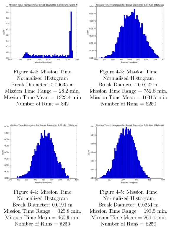
The histograms for the Mission Time values for each break size diameter are shown in Figures 4-2 to 4-9, respectively. The resulting range and mean values are shown in the caption of each figure.
Figure 4-2: Mission Time Normalized Histogram Break Diameter: 0.00635 m Mission Time Range = 28.2 min. Mission Time Mean = 1323.4 min
Number of Runs = 842
Figure 4-3: Mission Time Normalized Histogram Break Diameter: 0.0127 m Mission Time Range = 752.6 min. Mission Time Mean = 1031.7 min
Number of Runs = 6250
Figure 4-4: Mission Time Normalized Histogram Break Diameter: 0.0191 m Mission Time Range = 325.9 min.
Mission Time Mean = 460.9 min Number of Runs = 6250
Figure 4-5: Mission Time Normalized Histogram Break Diameter: 0.0254 m Mission Time Range = 193.5 min.
Mission Time Mean = 261.1 min Number of Runs = 6250
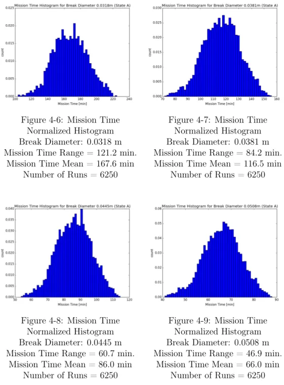
Figure 4-6: Mission Time Normalized Histogram Break Diameter: 0.0318 m Mission Time Range = 121.2 min.
Mission Time Mean = 167.6 min Number of Runs = 6250
Figure 4-7: Mission Time Normalized Histogram Break Diameter: 0.0381 m Mission Time Range = 84.2 min. Mission Time Mean = 116.5 min
Number of Runs = 6250
Figure 4-8: Mission Time Normalized Histogram Break Diameter: 0.0445 m Mission Time Range = 60.7 min.
Mission Time Mean = 86.0 min Number of Runs = 6250
Figure 4-9: Mission Time Normalized Histogram Break Diameter: 0.0508 m Mission Time Range = 46.9 min.
Mission Time Mean = 66.0 min Number of Runs = 6250
The probability distribution function of Mission Time values for a break diameter of 0.00635m (Figure 4-2) is roughly uniform until about 1330 minutes. After this, there is a sharp increase in the frequency of the Mission Time values. This is because the uniform values constitute the tail of the distribution. It is likely that the majority of the distribution values are above one day. However, more simulation runs for longer time periods than one day are necessary to make conclusions. A majority
of the simulation runs (5408 out of 6250) were discarded because the core was not uncovered from the coolant within one day from scram.
The distributions of Mission Time values for a break size diameters of 0.0127m to 0.0508m (Figures 4-3 to 4-9) are skewed to the left. The skew is a result of the propagation of the Low Pressurizer Pressure Trip Point (PPSL) uncertainty, which was modeled with a lognormal distribution. The higher the PPSL value is, the higher the pressure will be when the reactor scrams. This means that the coolant in the reactor will take longer to saturate because it is farther from the saturation pressure. Since Mission Time is calculated from the time at which the coolant is saturated to the time at which the core is uncovered from the coolant, if the saturation of the coolant is delayed then the total Mission Time will be shorter. Therefore, the skew to the right (higher pressures) of the lognormal PPSL uncertainty distribution is seen in the skew to the left (lower Mission Time values) in the distributions of the Mission Time values.
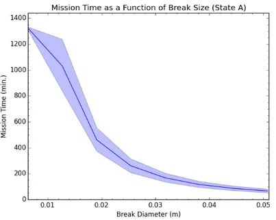
Figure 4-10 shows the dependence of Mission Time upon break diameter. The solid line shows the average of the runs and the shaded region represents the 90% interval of the runs. The 90% interval is reported so that the tails of the distribution, as well as any outliers, would be excluded from the interval. This allows the interval shown to more effectively describe the extend of the effect the TH uncertainties have upon the uncertainty in Mission Time values.
Figure 4-10: Mission Time as a Function of Break Size (Mode A
The Mission Time decreases as the break size increases. In addition, the range of Mission Times decreases as the break size increases. This is because as the break size increases, the speed of the transient increases. There is less time for the full effect of the uncertain parameters to be realized in the transient.
I calculated the probability of non-reconfiguration utilizing the three methods described in the beginning of the section. The dependences of the PNR values upon break diameter are shown in Figure 4-11.
Figure 4-11: P𝑁 𝑅|𝐶𝐼𝐶𝐴 (Mode A)
Each method resulted in the same PNR value of 0.01 until a break diameter of 0.0318m. As the break size increases, the PNR values were not the same for each of the three calculation methods. The second method (PNR with Uncertainties (Aver-aged)) appears to overestimate the PNR value and the first method (PNR without Uncertainties) seems to underestimate the PNR. The first and second methods are restricted to a PNR value of 0.01 and 0.1 because only one Mission Time value is utilized in the calculation of the PNR value in these methods. The PNR is restricted to the values in Equation 3.3. However, since all of the calculated Mission Time values are used in method 3, the PNR increases from 0.01 (all Mission Time values are above 90 minutes) as soon as there is at least one Mission Time value below 90 minutes, which occurs at a break size diameter of 0.0381m.
4.1.2
Mode B
Mode B is the operational state of the reactor during the first 6.5 hours after shut-ting down the reactor for a planned outage. Figure 4-12 depicts the Mission Time histogram obtained from a total of 38,097 runs in which the core was uncovered by the coolant within one day (1440 minutes) from the initiating event (SBLOCA). The
calculated Mission Time values range from about 30 minutes to one day.
Figure 4-12: Mission Time Normalized Histogram (Mode B)
The distribution in Figure 4-12 is also not unimodal. It appears to have two local extrema. Taking a similar approach to Mode A, I examined the Mission Time histograms for each of the eight break sizes: 0.00635m, 0.0127m, 0.0191m, 0.254m, 0.0318m, 0.0381m, 0.0445m, and 0.0508m. These are shown in Figures 13 to 4-20, respectively. The Mission Time range and Mission Time mean values are in the caption below each figure.
Figure 4-13: Mission Time Normalized Histogram Break Diameter: 0.00635 m
Range = 1215.1 min. Mission Time Mean = 240.8 min
Number of Runs = 2723
Figure 4-14: Mission Time Normalized Histogram Break Diameter: 0.0127 m
Range = 671.7 min.
Mission Time Mean = 1199.9 min Number of Runs = 862
Figure 4-15: Mission Time Normalized Histogram Break Diameter: 0.0191 m
Range = 1112.8 min. Mission Time Mean = 860.6 min
Number of Runs = 3919
Figure 4-16: Mission Time Normalized Histogram Break Diameter: 0.0254 m Mission Time Range = 1250.8 min.
Mission Time Mean = 661.6 min Number of Runs = 5604
Figure 4-17: Mission Time Normalized Histogram Break Diameter: 0.0318 m Mission Time Range = 1322.5 min.
Mission Time Mean = 491.0 min Number of Runs = 6236
Figure 4-18: Mission Time Normalized Histogram Break Diameter: 0.0381 m Mission Time Range = 1074.5 min.
Mission Time Mean = 338.4 min Number of Runs = 6250
Figure 4-19: Mission Time Normalized Histogram Break Diameter: 0.0445 m Mission Time Range = 767.2 min.
Mission Time Mean = 249.1 min Number of Runs = 6250
Figure 4-20: Mission Time Normalized Histogram Break Diameter: 0.0508 m Mission Time Range = 613.8 min.
Mission Time Mean = 189.1 min Number of Runs = 6250
Break diameter 0.00635 (Figure 4-13) shows a trapezoidal distribution function. There is volatility from Mission time values of 1150 minutes to 1250 minutes. Break diameter 0.0127 (Figure 4-14) shows an distribution function with a positive slope. The positive slope is likely depicting the tail of actual Mission Time distribution. More simulation runs for longer time periods than one day are necessary to make
conclusions. A majority of the simulation runs (5388 out of 6250) were discarded because the core was not uncovered from the coolant within one day from scram.
The remaining break diameters (Figures 4-15 to 4-20) show a distribution function with a negative slope. This is a result of the propagation of the uncertainty in the time at which the transient is initiated. The uncertainty distribution of the time at which the transient is initiated is uniformly distributed from the time of reactor shutdown until 6.5 hours after the time of the reactor shutdown. Throughout this time range, there is an exponential decrease in core thermal power due to decay heat. This is estimated utilizing Equation 4.3 [21],
𝑄 𝑄0
= 0.066𝑡−0.2, (4.3) where Q is the core thermal power, Q0 is the core thermal power at operation,
and t is the time since reactor shutdown. This is the exponential decrease that is seen in the Mission Time value distribution function. At the higher power, the transient moves more quickly and so the Mission Time value is smaller.
Like Mode A, the Mission Time values in Mode B are dependent on break size. Even considering the uncertainty in Mission Time, the slope has an overall negative value. Figure 4-21 shows the dependence on Mission Time on the break diameter. The solid line shows the average of the runs and the shaded region represents the 90% interval of the runs. The 90% interval is reported so that the tails of the distribution, as well as any outliers, would be excluded from the interval. This allows the interval shown to more effectively describe the extend of the effect the TH uncertainties have upon the uncertainty in Mission Time values.
Figure 4-21: Mission Time as a Function of Break Size (Mode B)
As with Mode A, the Mission Time decreases with increasing break size. However, unlike Mode A, the range of the Mission Times increases until the 0.0254m diameter break size and then decreases. The initial increase in the Mission Time range is due to the simulation cut off time of one day. Most of the Mission Times will be larger than one day for the smaller break sizes. The Mission Time range reported here only extends to one day and therefore excludes the upper part of the range. If the entire range were to be reported, then the Mission Time range likely would decrease with increasing break diameter, which is the same behavior as Case A.
I calculated the probability of non-reconfiguration utilizing the three methods described in the beginning of the section. The PNR values a functions of break diameter are shown in Figure 4-22.
Figure 4-22: P𝑁 𝑅|𝐶𝐼𝐶𝐴 (Mode B)
The PNR without Uncertainties method and the PNR with Uncertainties (Aver-aged) method both resulted in a uniform probability of non-reconfiguration of 0.01 across the break diameters. This indicates that both of these methods used a Mis-sion Time of over 90 minutes (from Equation 3.3). Therefore, the concluMis-sion from both of these methods is that the operator is unlikely to fail. However, the PNR with Uncertainties (Integrated) method shows a slight increase in the probability of non-reconfiguration for break diameters above 0.0381m. This is because the Mis-sion Times below 90 minutes that are the result of the uncertainty propagation are considered in the calculation of the PNR values.
4.1.3
Mode C
Mode C is operational state of a reactor during the time from 6.5 to 13.5 hours after shutting down the reactor for a planned outage. Figure 4-12 depicts the Mission Time histogram obtained from a total of 12,547 runs in which the core was uncovered by the coolant within one day (1440 minutes) from the initiating event (SBLOCA). The calculated Mission Time values range from about 180 minutes to one day.
Figure 4-23: Mission Time Histogram (Mode C)
The distribution in Figure 4-23 is also unimodal. It appears to have two local extrema. Each local extremum is associated with a reactor temperature condition (see Figure 3-1 for the temperature profile during shutdown). The local extremum at the upper Mission Time results from the two hours in Mode C that the reactor primary loop is at 170∘C. The local extremum at the lower Mission Time results from the one hour that the reactor primary loop is at 180∘C. The higher temperature causes the transient speed to increase.
Taking a similar approach as with Mode A, I examined the Mission Time his-tograms for six of the eight break sizes: 0.0191m, 0.254m, 0.0318m, 0.0445m, and 0.0508m. These are shown in Figures 4-13 to 4-20, respectively. The Mission Time range and Mission Time mean values are in the caption below each figure. The re-sults from the smallest two break diameters were not plotted because there were no simulation runs in which the core was uncovered from coolant within one day from the initiating event. Therefore, no Mission Time values could be calculated.
Figure 4-24: Mission Time Normalized Histogram Break Diameter: 0.0191 m Mission Time Range = 405.4 min. Mission Time Mean = 1258.5 min
Number of Runs = 121
Figure 4-25: Mission Time Normalized Histogram Break Diameter: 0.0254 m Mission Time Range = 816.7 min. Mission Time Mean = 1107.4 min
Number of Runs = 931
Figure 4-26: Mission Time Normalized Histogram Break Diameter: 0.0318 m Mission Time Range = 1037.6 min.
Mission Time Mean = 957.3 min Number of Runs = 1836
Figure 4-27: Mission Time Normalized Histogram Break Diameter: 0.0381 m Mission Time Range = 1160.6 min.
Mission Time Mean = 817.1 min Number of Runs = 2983
Figure 4-28: Mission Time Normalized Histogram Break Diameter: 0.0445 m Mission Time Range = 1233.2 min.
Mission Time Mean = 714.3 min Number of Runs = 3231
Figure 4-29: Mission Time Normalized Histogram Break Diameter: 0.0508 m Mission Time Range = 1254.5 min.
Mission Time Mean = 640.6 min Number of Runs = 3445
Break diameter 0.0191 (Figure 4-24) shows a sporadic distribution. This is due to the lower amount of simulation runs in which the core uncovered from coolant within one day (less than one percent of total simulation runs). More simulation runs are needed to refine this region of the distribution. The need for more simulation runs is verified with the variance analysis (see Appendix C, Figure C-17). The variance has not yet converged.
The remaining break diameters (Figures 4-25 to 4-29) show bimodal distributions. Each local extremum is associated with a reactor temperature condition (see Figure 3-1 for the temperature profile during shutdown). The local extremum at the upper Mission Time is from the two hours in Mode C that the reactor primary loop is at 170∘C. The local extremum at the lower Mission Time is from the one hour that the reactor primary loop is at 180∘C. The higher temperature causes the transient speed to increase.
As with Modes A and B, the Mission Time is strongly dependent upon the input of break size. Figure 4-21 shows the dependence of Mission Time upon the break diameter. The shows the mean Mission Time value of the runs and the shaded region represents the 90% interval of the runs. The 90% interval is reported so that the tails of the distribution, as well as any outliers, would be excluded from the interval. This
allows the interval shown to more effectively describe the extend of the effect the TH uncertainties have upon the uncertainty in Mission Time values.
Figure 4-30: Mission Time as a Function of Break Size (Mode C)
As with Modes A and B, the Mission Time decreases with increasing break size. The range of the Mission Times increases slightly as break size increases. This is because the transients with a larger break size have an increased speed. This means that more of the simulation runs at a lower pressure will have the core uncover form the coolant within one day. Less simulation runs were excluded and so the true range is being captured.
I calculated the probability of non-reconfiguration utilizing the three methods described in the beginning of the section. The PNR values as functions of break diameter are shown in Figure 4-22.
Figure 4-31: P𝑁 𝑅|𝐶𝐼𝐶𝐴 (Mode C)
Each of the three methods determined the probability of non-reconfiguration to be equal to 0.01 across the break diameters examined. This is because, as can be seen in Figure 4-23, there are no Mission Time values below 90 minutes (as per Equation 3.3). This means the operator is unlikely to fail to manually initiate safety coolant injection when the reactor is operating in Mode C.
4.2
Case 2
In Case 2, the operating crew tests for saturation of the primary system coolant before the saturated primary system state can occur during a SBLOCA. I assumed that this will occur if the Saturation Time (Equation 3.1) is above 3 minutes because I assume the operator will likely perform the saturation test within the first three minutes following scram [5] [22] . The mission is to realize the need to retest for the saturation of the primary system. The value of the probability of failing to realize this need is found as the probability of non-reconfiguration value (P𝑁 𝑅|𝐶𝐼𝐶𝐴 or PNR).
The PNR value is a function of Mission Time (Equations 3.2 and 3.4).
I present the results for Modes B and C. There are no simulation runs where Saturation Time is greater than 3 minutes in Mode A. Thus, this state is not plausible
for Mode A. I first present a histogram of the Saturation Time values for all runs which has a Saturation Time less than one day (1440 minutes). Then, for those runs that had a Saturation Time of greater than 3 minutes, I present a histogram of the Mission Times. For both Modes B and C, there are no Mission Times less than 50 minutes. So, the value of the probability of non-reconfiguration is obtained as 0.01 for all break sizes as per Equatino 3.4. Therefore, I concluded that there was no need to perform an independent analysis of each break size.
A Monte Carlo variance analysis was performed for the Saturation Time distri-bution for Modes B and C. This was performed in order to verify that adequate runs were performed and that undersampling did not occur. I performed this analysis by calculating the variance of the distribution of Saturation Time as a new Saturation Time value from each simulation run was added. As my modeled distribution of Sat-uration Time values approaches the real distribution, then the change in the variance value of the Saturation Time distributions approaches zero. I show the plots of the percent change in the Saturation Time distribution variance values as function of the simulation runs for Modes B and C in Appendix C.
4.2.1
Mode B
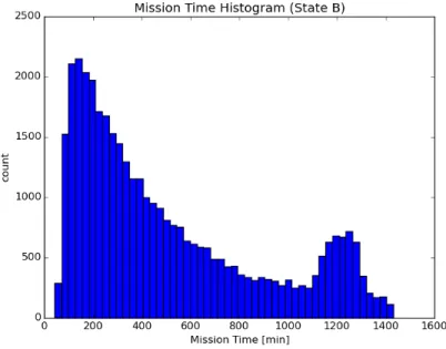
Figure 4-32 shows a histogram of the Saturation Time results for the N = 38,097 simulation runs. If the Saturation Time is greater than 3 minutes, I assume that the operator will not observe the saturation conditions.
Figure 4-32: Saturation Time Histogram (State B)
The Saturation Time histogram has three visible local extrema. Each local ex-tremum is a result of the different break sizes. The local exex-tremum for the smallest Saturation Time is that of the largest break size. The amplitudes of the following local extrema are lower because the range is larger for the smaller break sizes and so the distributions have a larger spread. The histogram is normalized for each break size.
A total of 29,507 runs out of the 38,097 simulation runs had a Saturation Time above 3 minutes. A histogram of the Mission Times for these runs is in Figure 4-33