Advanced techniques for flutter clearance

Advanced Techniques for Flutter Clearance

by

Laurent Guillaume Duchesne

Submitted to the Department of Aeronautics and Astronautics

in partial fulfillment of the requirements for the degree of

Master of Science in Aeronautics and Astronautics

at the

MASSACHUSETTS INSTITUTE OF TECHNOLOGY

January 1997

@

Massachusetts Institute of Technology 1997. All rights reserved.

A uthor ...

Department of Aeronautics and Astronautics

January 17, 1997

C ertified by ... .. ....

I

...

Eric Feron

Assistant Professor

Thesis Supervisor

Accepted by ...

Jaime Peraire

Chair, Graduate Office

FEi; 1 0 197

... ....

Advanced Techniques for Flutter Clearance

by

Laurent Guillaume Duchesne

Submitted to the Department of Aeronautics and Astronautics on January 17, 1997, in partial fulfillment of the

requirements for the degree of

Master of Science in Aeronautics and Astronautics

Abstract

In this thesis, a new methodology for flutter boundary prediction using experimental data is developed. Due to the complexity of the aircraft's structure and aerodynamics, it appeared necessary to rely on a simplified wing model to create a low order state space representation that would capture all the essential dynamics of a flutter prob-lem. The methodology is the following: first, a low order finite element model was derived using linear aerodynamic theory and a Pade approximation. The technique also relies on a time-frequency analysis which selectively eliminates noise from the recorded signals in order to estimate the transfer function of the system. A graphical interface was developed to perform this task more efficiently. Then, a state space model parameterized by the dynamic pressure q is identified with a quasi-Newton optimization based on a frequency domain cost function. Finally, the flutter bound-ary is determined based on the domain of stability of the parameterized model. This methodology has been validated first on a theoretical example, then on wind tunnel data through the Benchmark Active Controls Technology (BACT) model and finally on the F18 System Research Aircraft.

Thesis Supervisor: Eric Feron Title: Assistant Professor

Acknowledgments

First of all, I would like to thank my advisor Eric Feron for the interest and enthusi-asm that he has showed throughout my stay at MIT. I would also like to thank Jim Paduano who acted as a co-advisor for this project. I wish to acknolewdge all the NASA Dryden Flight Research Center engineers with whom I have interacted with a special thank to Marty Brenner with whom I have shared many productive discus-sions. Finally, I would like to thank all my lab mates who provided useful advice and more importantly friendship.

This work was supported by NASA under the Consortium program NCC 2-5116 entitled "Advanced Techniques for Flutter Clearance" and the cooperative research agreement DFRCU-95-025 entitled "Methods for In-Flight Robustness Evaluation".

Contents

1 Introduction 11

1.1 M otivation . . . . . . .. . . 11

1.2 O utline . . . . 12

2 Classical flutter boundary determination 15 2.1 Typical section dynamics ... 16

2.2 Aerodynamic model ... ... 17

2.3 Classical flutter prediction ... .. . . 20

3 Classical identification techniques 23 3.1 Parameter estimation method ... ... 23

3.2 Subspace identification ... 26

3.2.1 Notations ... 26

3.2.2 Step by step procedure ... ... 28

3.3 Multiple data sets in subspace identification . ... 29

3.3.1 Motivational example ... .... 30 3.3.2 A lgorithm . . . . 33 3.3.3 R em arks . . . . 34 3.3.4 Exam ples . . . 35 3.4 Conclusion ... .... ... ... 41 4 A new methodology 43 4.1 Transfer function estimation ... .... 43

4.1.1 Principle of the estimation . . . . . 4.1.2 Resolution issues ... 4.1.3 Graphical interface . . . . 4.2 Identification ... 4.2.1 Model definition ... 4.2.2 Cost definition ...

4.2.3 Estimating the physical parameters

5 Application to wind tunnel data (BACT model)

5.1 Presentation of previous research . ... 5.2 Identification of the BACT model . ...

6 Application to the F18-SRA

6.1 Description of the experiment . . . 6.2 Data analysis ...

6.3 Transfer function estimation . . . .

6.4 Description of the structural model 6.5 Evaluation of the C matrix . . . . . 6.6 Evaluation of the A matrix . . . . . 6.7 Flutter results ...

7 Conclusion

A Linearized equation of motion of a typical wing section B State space model example

C Gradient of the cost function used in the identification procedure

. . . . . 45 . . . . 48 . . . . . 49 . . . . 49 . . . . 50 . . . . 5 1 . . . . . 52 65 . . . . . 65 . . . . . 68 . . . . . 74 . . . . . 76 . . . . . 78 . . . . . 80 . . . . . 82

List of Figures

2-1 Typical section of the airfoil .. . . . ... . . . .. 17 2-2 Root locus of the flexible aircraft with respect to air speed ... 21

2-3 Evolution of the damping ratio and the real part of the torsion mode of the aircraft with respect to air speed. . ... 22

3-1 Concatenation of two simulations made on a 8th order system with two

different inputs and no noise. . ... ... 31 3-2 Simulation made with the same system as in Figure 3.1 but with the

concatenated input ... ... 32

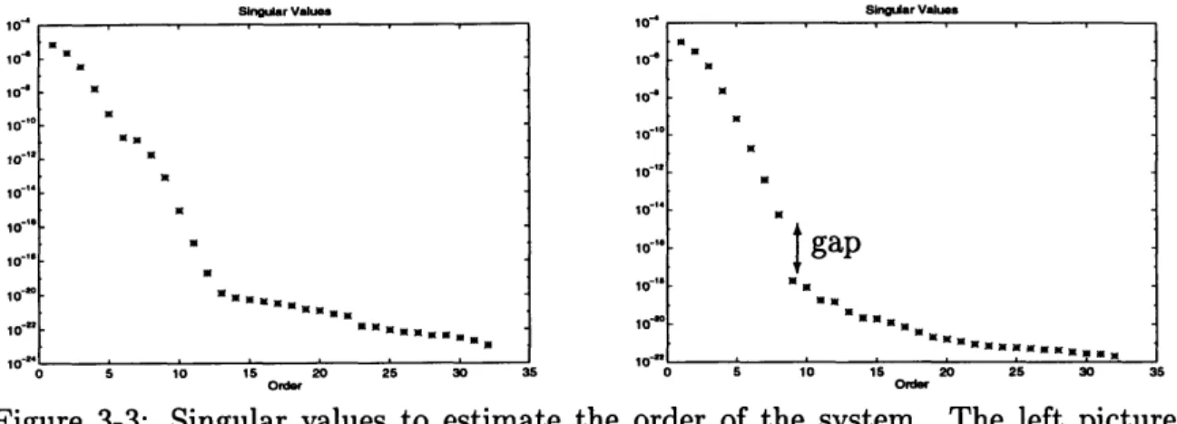
3-3 Singular values to estimate the order of the system. The left picture happens when concatenating the data, the right one is with the new

scheme. ... ... ... ... 33

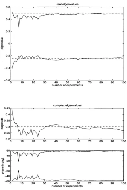
3-4 Identified eigenvalues with respect to the number of experiments for a

stable system ... ... ... 37

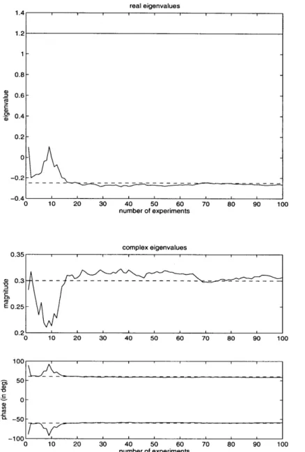
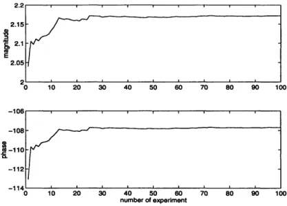
3-5 Identified eigenvalues for an unstable system. . ... 38 3-6 Convergence of the short period eigenvalue for the steady state case.. 39

3-7 Evolution of the short period eigenvalue with respect to time in a pull

up maneuver. ... ... ... 39

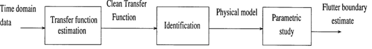
4-1 Flowchart of the methodology . ... . . . . . 44

4-2 Choice of the parameters N1 and N2 of the input and output signals . 46

4-3 Signal representation using the graphical interfacing tool ... . 49 4-4 This plot shows how the flutter boundary prediction evolves with

5-1 Measure of the accuracy of flutter prediction of the BACT model using

analytical data . ... ... 62

5-2 Measure of the accuracy of flutter prediction of the BACT model using

experimental data. ... 63

5-3 Flutter boundary prediction in a Mach vs dynamic pressure diagram 63 6-1 Diagram of the DEI exciter ... .. 66 6-2 Aerodynamic force due to the DEI exciter with respect to its position. 67 6-3 Diagram of the F18-SRA with the DEI exciter . ... 68 6-4 Flight envelope of the F18 and flight conditions at which experiments

were perform ed ... ... 69

6-5 Plot of the coherence of the input and output data at Mach 0.8, 10,000 feet . . . .. .. . 70

6-6 Transfer function estimate at Mach 0.8 and elevation of 10,000 feet 75 6-7 Typical transfer function fit ... 79 6-8 Normalized standard deviation vs. mean of the coefficient of C . . .. 80 6-9 Normalized standard deviation vs. mean of the coefficient of A . . .. 81 6-10 Flutter boundary prediction points . ... 82

List of Tables

3.1 Eigenvalues of the identified model. ... . 32

6.1 Position of the accelerometers ... ... 67 6.2 Coherence between the right exciter and the five first accelerometers . 71 6.3 Coherence between the right exciter and the five last accelerometers . 72 6.4 Flight condition for each data set . ... . 73

Chapter 1

Introduction

1.1

Motivation

Flutter is a phenomenon which is very critical in aeronautical engineering and arises in the design of the wings and the tail of an aircraft. It involves a coupling between inertial, structural and aerodynamic forces. Under certain conditions, typically in the transonic region or at high dynamic pressure, the combination of these three forces may create a self excited system that becomes unstable. Flutter therefore must be avoided on any aircraft because its presence can result in the yield of the structure. Furthermore, with the rise of new types of structures, wings are becoming more and more flexible thus bringing flutter boundary even closer to normal operating condi-tions. A more critical point is that, even though flutter boundary can be estimated in the design procedure of an aircraft, the results are not very reliable and a large margin of error must be allowed for. Therefore, flutter clearance is an essential part of the aircraft certification problems which has to be accomplished through extensive and expensive flight tests. The goal of this thesis is to provide efficient and reliable ways to predict flutter boundary in real-time by using recorded flight data.

The wing flutter problem has been heavily studied in the past, and its theoretical development, based on linear aerodynamic theory, can be found in [9] and [37]. A Pade approximation is also used to model some delays in the aerodynamic forces.

improved flutter boundary estimations. Currently, the so-called p-k iteration [13] is used to predict the flutter boundary. This algorithm actually solves finite element equations and gives an estimation of the damping ratio of each mode, given a specific flight condition. Then, an iteration on the flight condition needs to be made to find the flutter boundary. The preceding methods rely essentially on analytical computations and also on assumptions about the accuracy of linear aerodynamic theory. Indeed they do not take into consideration any flight measurements. In the past, experimental data have been used to clear operating points in the flight envelope from flutter but little extrapolation to the flutter boundary was attempted [3]. Lately, some attention has been given to the use of modern control theory such as robustness analysis in the prediction of flutter boundary . In [11], a methodology to obtain a conservative bound of flutter for an airfoil in a wind tunnel is developed. The problem was set up as a real-p problem with two uncertainties, Mach number and dynamic pressure. The same idea was adapted to the F18-SRA [21] where unmodeled dynamics were incorporated into the uncertainty as well.

1.2

Outline

Classical flutter boundary determination for a typical wing section is described in Chapter 2. The equations of motion are first derived and the flutter boundary is estimated using a damping ratio extrapolation. As further explained, this method may provide poor performance when the recorded data are taken at flight conditions that are not very close to the flutter boundary.

In Chapter 3 a review of major classical system identification techniques is pro-vided since it quickly appears as one of the critical points in a flutter clearance

problem. A short description of parametric identification methods is given but more attention is devoted to subspace identification methods. It is also shown how such methods can handle multiple data sets.

The overall procedure proposed in this thesis is developed in Chapter 4. A tech-nique based on time-frequency analysis is described to estimate the transfer function

of the system based on frequency sweep excitation signals. A Newton optimization algorithm is then used to identify the system at different flight points simultaneously. A validation of this method is done using the model described in Chapter 2 since it represents the dynamics of the flutter phenomenon very well.

Application of the identification technique to the BACT model in a wing tunnel experiment was achieved. The flutter boundary determination was duplicated from earlier work by K. Gondoly based on robustness analysis. Improvements of results obtained with experimental data is also presented.

Finally, the proposed procedure is applied to the F18 SRA and described in Chap-ter 6. The flight data were provided by NASA Dryden Flight Research CenChap-ter and the experiments included flight conditions at different altitudes (10,000 30,000 and 40,000 feet) and different Mach numbers in the transonic region (Mach 0.8, 0.85, 0.9 and 0.95).

Chapter 2

Classical flutter boundary

determination

Although a real aircraft is not strictly speaking a single elastic unit, it is necessary

from an engineering view point to treat it as such in order to deal with the complexity of flutter problems. Another simplification is to limit the study to a specific part of the aircraft that is susceptible to generating unstable oscillations. In general, an aircraft has two critical points, the wings and the tail, and it is usually assumed that there is no interaction between those two parts of the aircraft. In this thesis, only the wing flutter problem will be addressed.

It is also necessary to make some further assumptions because, even if the wing is considered as a cantilevered structure, it would still be a continuous system which has an infinite number of modes. Since this is unfeasible in practice, a finite element model is usually derived from the geometry and the material of the aircraft. However, to understand the most important part of the physics involved in a flutter problem, a typical wing section is enough [9]. In this Chapter, only a simple typical section is presented to allow the reader understand the flutter phenomenon.

2.1

Typical section dynamics

Let us consider a unit width strip of a two-dimensional flat plate airfoil which has two degrees of freedom: a bending mode and a torsion mode (also called pitching mode). As a convention, a positive bending h will be downward, and a positive torsion a will be pitching up. The semi-chord of the airfoil is denoted b, and the ratio of the distance between the elastic axis and the center of gravity to the semi-chord is ah. The x-axis is defined to be parallel to the air speed U. The model and the notations are illustrated in Figure 2-1. Note also that two springs were incorporated in the system to model the strain due to the rest of the wing. For an elementary unit length dx on the x-axis, the small element of the airfoil has an elementary mass denoted dm. The kinetic energy of an element of mass at a distance x from the elastic axis is

dT = (h + x&)2dm. (2.1)

So, the kinetic energy of the typical section is

1

T = -(mh 2 _{+ 2Sh& + I,&2), (2.2)}

2

where m is the mass per unit span of the wing, S, is the static moment of inertia about the elastic axis and I is the mass moment of inertia about the elastic axis. Those terms can be computed using the following expressions:

nm =

dm,

S,= xdm,

S= J 2dm.

If the stiffness of the bending and torsion spring are respectively defined as kh and

u kh h

a --- -- ....--

---ka

b.ah

b

Figure 2-1: Typical section of the airfoil.

1 1

U= khh2 + -k a2. (2.3)

2 2

Since the gravity does not play a fundamental role in the flutter phenomenon, this force was omitted in the formula for the potential energy for reasons of simplicity. The Lagrange equation of motion can now be computed

mh + S& + khh = -L (2.4)

SI + I,& + ka = M, (2.5)

where L and M represent respectively the aerodynamic force and moment about the elastic axis.

2.2

Aerodynamic model

Proceeding further in the derivation of the equation of motion, the description of the aerodynamic forces needs to be performed. The theory that will be considered is called linearized aerodynamic theory. It assumes that all the forces and moments are linear with respect to the air density p. The forces can be decomposed into two parts: the non-circulatory and the circulatory one.

of gravity to the elastic axis and the chord, and U as the airspeed, the lift of the non-circulatory part can be decomposed as follows:

1. A lift force with center of pressure at the mid-chord

L1 = pb2 (h - ahbo) (2.6)

2. A lift force with center of pressure at -chord point

L2 = pirb2U& (2.7)

3. A nose down moment

prb4

Ma= a8 (2.8)

For the circulatory part, the step response to a vertical velocity component w (or downwash) was obtained by Wagner, Kussner, von Karman and Sears and is equal to

L3(T) = 27rbpUw(rT), (2.9)

where 7 = Ut/b is non-dimensional quantity proportional to the time t. The function

1D is called the Wagner's function. It is a highly nonlinear function but can, however,

be approximated by

(7T) = 1 - 0.165e-0.041_{7 - 0.335e-0}32

_r.

_(2.10)

The downwash due to the two degrees of freedom h and a consist of the three following terms:

1. A uniform downwash corresponding to a pitching angle a, w = U sin a = Ua 2. A uniform downwash due to vertical translation h

In the interval [ro, o + tTo], the downwash w(To) increases by an amount d(o)dTo.

When dro is sufficiently small, this may be regarded as an impulsive increment and the corresponding circulatory lift is

dL3(T) = 27rbpU((7 - Todw) dro.

tTo

By the principle of superposition, the circulatory lift becomes

L3 = 27rbpU D(T - To)w(To)dTo. (2.11)

oo TO

The total lift on the on the typical section is

L = LI + L2 + L3, (2.12)

and the total moment about the elastic axis is

1 1

M = ( + ah)bLl + ahbL₂ - (- - ah)bL+Ma. (2.13)

2 2

Since the Wagner's function is a function of 7, it is convenient to convert the equation of motion and use r instead of t as the time variable. To do this, we need to relate the differentiation of a function f with respect to the physical time

f

to the differentiation with respect to the non dimensional time f':

df df dT Uf

f- _{dt dr dt b}f'. (2.14)

Using this notation, the aerodynamic lift and moment about the elastic axis in-duced by h and a are

L(T) = 2rbpU2

L

( - To)[a'(To) + b "(To) + ( - ah)a(T)]dTo

+pr U2_{(h" - ahba") + prbU}2_{a' (2.15)}

1 1 1

M(T) =(- + ah)2rb2pU2 00 (T - To) [a'(To) + h"(To) + ( - ah)a"(To)]dro

+ahbprU2 (h - ahb") ( - ah)pr b2U2 Prb2U2 . (2.16)

2 8

Using this notations, the full equation of motion using the dimensionless time is

U2 U2

m -h" + S a" + mwh2h = -L(T) (2.17)

U2 U2

S h" + I- a + IWQ2 = M(T), (2.18)

where Wh = kh/m and w, = kI.

2.3

Classical flutter prediction

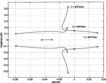
The equations that have been derived model a self-excited system. Flutter occurs when the state space model becomes unstable. Since the equations are linear, the stability is checked by calculating the poles of the system. This is simple to do once the model has been converted to a state space format, since it becomes an eigenvalue calculation. However, to write the equation in a matrix form, it is important to notice that the Wagner's function introduces some exponential terms in the time domain. Those terms can be dealt with by adding two states to the system, which are usually called the lags. The derivation of the state space model is shown is Appendix A. Once the geometry of the wing is specified, the state space matrix A becomes a function of air density p and air speed U only. It is interesting to plot the evolution of the eigenvalues of the A matrix with respect to one of the two variables, the other one remaining constant. Such a plot is called a root locus, and an example is shown in Figure 2-2. In this case, the air speed varies from 200 ft/sec to 500 ft/sec. Notice that the aircraft structure becomes unstable for air speed greater than 429 ft/sec. This instability point, marked with a star on the figure, is the flutter boundary point that we are interested in.

U 200 ft/sec 0.4 0.3 0 .2 . . . .. . . . ... .... ... U. 9.sec .. ..42 -0.2 -0.3 -0.08 -0.06 -0.04 -0.02 0 0.02 0.04ft/sec real part

Figure 2-2: Root locus of the flexible aircraft with respect to air speed.

As stated in the introduction, the problem addressed in this thesis is to predict the flutter boundary based on flight data that are necessarily taken in the stable region of the structure. Therefore, it is not possible to obtain the root locus of the

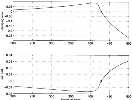
flexible structure close to the flutter boundary. The solution is then to extrapolate the results that were obtained at lower air speed or lower air density up to the point of instability. Let us assume, at first, that the poles of the system can be calculated exactly by using some identification techniques. It is then possible to calculate the error that is made by extrapolating the poles to higher speed. To obtain an idea of the accuracy of the results, let us plot the real part as well as the damping ratio (which has more physical meaning) of the pole that is going unstable with respect to speed (Figure 2-3). Notice that the change of behavior of this parameter is very abrupt in the neighborhood of the flutter boundary. This means that the extrapolation will

give an accurate answer only when the air speed of the point at which the poles are calculated is very close to the boundary, typically on the right side of the dashed line. In other words, to obtain a reliable answer by extrapolating the damping ratio of the

pole, we need to know a priori the answer with an uncertainty of less than 4%. An a priori estimate of the flutter boundary can be obtained by a finite element modeling of the aircraft and aerodynamics. However, the results would usually not be accurate of the aircraft and aerodynamics. However, the results would usually not be accurate

0 -0.05 -0.1 -0.2 0.25 -200 250 300 350 400 450 500 0.04 0.03 -_{0 .02 .... ....} ..._{. . .... ... ... ... ... .... ... ....} 0.02 - _{i ... .... ... ...} 0 . . -0 .0 1 . ... ... ... .. .. -0.02 i i 200 250 300 350 400 450 500

Speed (in ft/sec)

Figure 2-3: Evolution of the damping ratio and the real part of the torsion mode of the aircraft with respect to air speed.

enough to allow the use of such a method. The noise was not taken into account up to this point of the analysis. In real life, noise can never be avoided, providing even more uncertainty in the results. This is amplified by the fact that we need to evaluate the derivative of a curve to predict flutter, which is usually very sensitive to noise.

It was shown, in this section that extrapolating the damping ratio with respect to the air speed or the air density is accurate only when data is available close to the flutter boundary. In practice, this constraint is very limiting because flying close to the instability region is very dangerous for the pilot. Another problem is that the flutter boundary is originally unknown, so in order to fly close to it, it may require many expensive flight tests. An alternate method, explained in Chapter 4, is necessary to solve this problem.

Chapter 3

Classical identification techniques

In this thesis, the goal is to predict flutter boundary by relying heavily on recorded data. The general idea is to obtain an accurate state space model of the structural dynamics of the aircraft that is in agreement with both flutter theory and experimen-tal data. Therefore, an essential step of the procedure is system identification. This topic has been extensively studied in the past and a fairly comprehensive survey of existing methods can be found in [23]. The main techniques are described briefly in this chapter but special attention is devoted to subspace identification. Some inter-esting contributions on data sets combination are also described in detail, illustrated by a series of applications.

3.1

Parameter estimation method

The first step of a parameter estimation method is to define a model which is in accordance with the physics of the system to identify. Many different models have been proposed in the past. The most popular one is the Auto Regressive Model (ARX) which is presented briefly. The general ARX model has the following form:

na nb

y(t) = 1 Aky(t - k) + L Bku(t - k) + n(t), (3.1)

where y is the output, u the input and n the noise. na and nb are two integers that respectively represent the order and the number of zeros of the model. Those two numbers are chosen by the user based on physical knowledge on the system. However,

nb should be smaller than na to get a strictly proper system. The other parameters, Ak and Bk, are constants to evaluate through the identification method. Writing Equation (3.1) in a matrix form leads to

... " Yna Una-nb+1 ... Yp-1+na _Up+na-nb Una Up-l+na A1 Ana B₁ Bnb

I

Yna+1 - nna+l Yp+na - np+na

where p is an index for the number of data samples. Equation (3.2) is a set of linear equations in Ak and Bk that are solved through a least square method.

... " " Yna Una-nb+l1 ... Yp-1+na Up+na-nb Un_a Up-l+na Yna+l - nna+1 (3.3) Yp+na n- P+na

assume that the noise is white, with zero mean and a variance of a,2, we that the estimate is unbiased, since the expected value of the error e equals

-t

1 .. " Yna Una-nb+1 . na

E(e) = " E(n) = 0

Yp " Yp-1+na Up+na-nb Up-l +na

(3.4) Y1 Yp (3.2) YI

Lp

A1 Ana B1 Bnb Bnb If we can note

Denoting

-t Y1 " " Yna Un-nb+1 Una

Q

, (3.5)

Yp " " Yp-l+na Up+na-nb Up-l+na

The variance a2 _{of the estimate is}

a2 _{= E(eeT) = a}2_{QQT (3.6)}

Note that the variance of the estimate is linked to the singular values of the matrix

Q. _{The variance can be decreased by increasing the amplitude of the input signal,}

which means adding more energy to the system. This assertion is true as long as non-linearities in the system can be neglected which implies magnitudes of the input signal to be small. Therefore, there is a trade off.

Other types of model can be found in the literature such as the Auto Regressive Moving Average Model (ARMAX), Output Error models (OE), Finite Impulse Re-sponse models (FIR) or the Box-Jenkins models (BJ). A more comprehensive list can be found in [24, 23]. Each model assesses some properties on the system such the

number of modes or the properties of the noise. For example, the ARMAX model has the following structure

na nb nc

y(t) = Aky(t - k) + Bku(t - k) + C Ckn(t), (3.7)

k=1 k=1 k=1

where some dynamics are added to the noise.

Other types of model assume that the input is an unknown noise having some known properties. For example, the Auto Regressive Model (AR) is the following

y(t) = E Aky(t - k) + n(t), (3.8)

k=1

Methods to identity such models are usually called prediction methods and those problems are addressed in [25, 2].

3.2

Subspace identification

Subspace identification methods have been initiated by the works of Kung [19], and Juang and Pappa [17]. A variety of new methods have emerged ([31], [28], [4] and [22]) for identifying a system in the time domain, [32] for systems with stochastic input, and also [26] in the frequency domain. Efficient numerical procedures using the structures of Hankel and Toeplitz matrices, saves computational time and storage, increasing the performances of such algorithms [5]. All those methods are based on the same basic principle, presented in this section through a simple subspace identification algorithm.

3.2.1

Notations

The goal of subspace identification is to find a linear, time invariant, finite dimensional state space realization

Xk+1 = Axk + Buk (3.9)

Yk = CXk + DUk,

where A E nx, B E Rnxm, C E Rlxn, D E Rlxm, based on the knowledge of specific

sequences u = [u, ... , up], y = [Y1, ..., yp].

The following notation is used:

The block Hankel input and output matrices are defined as

Yk Yk+1 ... Yk+j-1

Yh(ki, j) = k+1 Yk+2 ... Yk+j

Yk+i-1 Yk+i ... Yk+j+i-2 and

Uh(k, i,

j)

=

Uk Ukc+1 .. Uk+j-1

Uk+1 Uk+2

Uk+i-1 Uk+i

We also introduce the extended observability matrix

C CA

CA'-the lower block triangular Toeplitz matrix

HtL = D CB CAB 0 D CB

CAi-2B CAi-3_{B CAi-}4_B and the state matrix

X=[ _{xk Xk+1} --. _{Xk+j-1 ]}

This notation leads to the following representation of the input output history:

Yh(k, i, j) = FX + HtUh.

... _Uk+j

... Uk+j+i-2

3.2.2

Step by step procedure

The step by step procedure of a subspace identification algorithm with one data set is now explained through the example of the deterministic identification (i.e. no noise is corrupting the data).

Step 1: find a matrix P that satisfies an equation of the form

P = FQ, (3.11)

where r is the extended observability matrix and such that rank(P)=rank(F)=n. In practice, the existence of noise makes it impossible to obtain equation (3.11) ex-actly. Any subspace method extracts a matrix P from the input to output data that is optimal in the sense defined by the method: the specific solution depends mainly on the noise assumption. Depending on the subspace method that is chosen, different computations of this matrix P are possible, all leading to different results.

In the case of a deterministic system, P can be found by post multiplying equa-tion (3.10) by a matrix Uh' that satisfies UhUh = 0. We then obtain P = YhUh- . However, the rank of the matrix P may not be equal to the order of the system. This phenomenon is known as rank cancellation and its probability of occurring decreases when the number of rows in Yh increases.

Step2: perform a singular value decomposition of P

P = USV,

where S = S 0 and U = (U1 U2) such that U1 is the first n columns of U. Note that S1 is an n x n matrix. With Equation (3.11), we can see that there must exist a full rank n x n matrix T such that

U = FT.

will be the matrix with a reduced number of rows, obtained from M by omitting the first (resp. last) 1 rows, where 1 is the number of outputs of the system.

Step 3: Evaluate A and C as follow: A = U1 tUi and C is equal to the first block of Ui, where U1t denotes the pseudo-inverse of U1 .

Using the structure of the extended observability matrix, it is clear that

F=FA

U1 = ET , U = FT

UIT- 1 = UIT-1A.

This can also be written as

U1 = UI J', ' = T-1AT.

Thus, I is a matrix similar to A, which is what we wanted originally. Step 4: Use a least square method to compute B and D.

We can pre multiply equation (3.10) by F' such that F'F = 0, and post multiply it by the pseudo-inverse of Uh. By using the structure of the matrix Htj, we get

r±YhUht = rl

D1

B leading to

D

D = (F' B

)

tFYlyhUht

3.3

Multiple data sets in subspace identification

Currently available time-domain subspace identification algorithms assume that plant identification is based on a single experiment, where only a single input to output data

set is available. There are, however, many cases for which data collection cannot be done all at once, and experiments must be segmented possibly over a period of several days, leading to the collection of many data sets all related to the same dynamic system, but with possibly different initial conditions. This is typically the case, for example, when attempting to identify the flexible dynamics of the F18 Systems Research Aircraft (SRA) at NASA Dryden Flight Research Center, where several data sets generated through many flights at the same flight conditions (altitude, Mach number and dynamic pressure) are available.

The idea of combining data sets into one single identification method is not new (see [20]). However, it has never been implemented on subspace identification meth-ods. In this section, it is shown how such an algorithm may be readily adapted to handle multiple data sets.

3.3.1

Motivational example

Before we start presenting the algorithm with multiple data sets, an example is first described to show that naive concatenation of the data sets leads to severely degraded performance. Results are compared with a method described in Section 3.3.2 and in [7] which recovers the original performance of subspace algorithms.

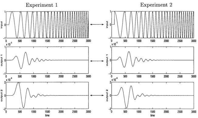
The system is an 8th _{order discrete time system with one input and two outputs,} whose state space representation can be found in Appendix B. The system has been excited separately by two sets of linear frequency sweeps. The choice of such inputs has been motivated by some practical concerns since frequency sweeps were the only available excitations at our disposal to identify the structural dynamics of the F18-SRA. The following formula for the inputs has been used from k = 100 to 3000, the first 100 points were set to zero:

el(k) = sin(27r(5 + 20k/3000)(k - 100)/3000) e2(k) = cos(27r(5 + 20k/3000)(k - 100)/3000).

Experiment 2 -1 -1 0 500 1000 1500 2000 2500 3000 0 500 1000 1500 2000 2500 3000 x 10 x 10 0 0 -1 -1 0 500 1000 1500 2000 2500 3000 0 500 1000 1500 2000 2500 3000 x10 x 10 2 2 o -21 -2 0 500 1000 1500 2000 2500 3000 0 500 1000 1500 2000 2500 3000 time time

Figure 3-1: Concatenation of two simulations made on a 8th order system with two

different inputs and no noise.

sets were concatenated. The plot of the input and outputs can be seen in Figure 3-1. Notice that the discontinuity at the junction of the two data sets is very small. Then, the identification of the system with a subspace algorithm (we used N4SID which is a state of the art method) was performed as if the concatenated data had been recorded from only one experiment. The number of blocks i in the Hankel matrix was set to 14, 15 and 16. For i = 15, the original system was perfectly recovered. The problem came when i = 14 or 16 was used since some of the eigenvalues have become unstable as seen on Table 3.1. Other values of i have been tested from 10 to 30 and the algorithm failed in about 70 % of the cases. Even though the identification was accurate for some values of i, the issue remains; the user has no way to discriminate between the right answer and the wrong one.

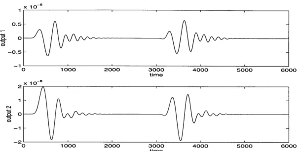
On Figure 3.3.1, the simulation of the system with the input concatenated is realized, and the outputs of this single experiment are plotted. By comparing those outputs to the one shown on Figure 3-1, it can be noticed that the difference between the two tests is very small. However, when applied to these data, N4SID recovered the

x 10 - s 0.5 -0.5 -- 1 0 1000 2000 3000 4000 5000 6000 time x 10 - 6 -1 20 1 oo 2o000 3000 4000 _5000 6000 time

Figure 3-2: Simulation made with the same system as in Figure 3.1 but with the concatenated input.

original eigenvalues calculated eigenvalues calculated eigenvalues by concatenating the two sets with this new algorithm

i = 14 i = 16

0.9893 + 0.0396i .9977+.0100i 1.0133 + 0.0614i 0.9893 + 0.0396i 0.9893 - 0.0396i .9977-.0100i 1.0133- 0.0614i 0.9893 - 0.0396i 0.9799 + 0.0245i .9960+.0200i 0.9969 + 0.0377i 0.9799 + 0.0245i

0.9799 - 0.0245i .9960-.0200i 0.9969 - 0.0377i 0.9799 - 0.0245i 0.9949 + 0.0149i .9944+.0386i 0.9985 + 0.0098i 0.9949 + 0.0149i

0.9949 - 0.0149i .9944-.0386i 0.9985 - 0.0098i 0.9949 - 0.0149i

0.9753 .9454+.1431i 0.9976 + 0.0195i 0.9754

0.9851 .9454-.1431i 0.9976 - 0.0195i 0.9850

Table 3.1: Eigenvalues of the identified model

right eigenvalues regardless of i. This shows that the identification procedure is very sensitive to data corruption.

To show that this problem does not come from the kind of input that has been chosen, the system was identified with each data sets separately. The original system was recovered with any i that we picked for both data sets.

N4SID was then adapted to handle multiple data sets, using the algorithm de-scribed in the next section. This modified version was used on the same numerical data. As shown in table 3.1, the result of this identification was very accurate. The eigenvalues were fitted with an error lower than 0.1%.

Sinmuiar Values 10 10 to 10 10~" m 10-1 10= C U 10- 10 10 gap to' t1 " 0 5 10 15 20 25 30 35 0 5 10 15 20 25 30 35 Order Order

Figure 3-3: Singular values to estimate the order of the system. The left picture happens when concatenating the data, the right one is with the new scheme.

The question of determining the order of the system is also a major issue in

identifi-cation methods. In practice, the order is also unknown and needs to be determined. In many subspace identification algorithms, the singular values of the matrix P (step

1) are plotted and the user must decide the order of the system. If there is a jump in the amplitude of the singular values, the order is determined by the number of singular values to the left of this jump. If there is no detectable jump, then the user must guess the system's order, based on his or her knowledge of the system. Figure 6 shows the plots that are obtained using both procedures with 16 blocks in the Hankel matrix (i = 16). Notice that it is not obvious to determine the order of the system when the data has been concatenated. On the other hand, there is a gap of 3 orders of magnitude for the improved procedure.

3.3.2

Algorithm

We will now assume that we have collected two data sets (the generalization to n data sets is very simple and is omitted for notation purposes), ul (k), yl (k) and u2(k),

y2(k) and the following equations are satisfied

Y = PX 1 + HUI (3.12)

Y2 =

rX

2

+

HU2.

Let us now explain how the original algorithm has to be modified in order to handle multiple data sets.

Step 1: Find two matrices P1 and P2 that satisfy Pi = FQi, for i = 1, 2, where P is the extended observability matrix.

Actually, this step is similar to the first step of the initial algorithm, but we need to perform it for each data set. For example, if we want to use the noise free method, we should proceed as follow

Pi = YU1I = r(X ₁U1 )

P2 = Y2U21 = F(X2U2 ).

The main modification of the algorithm is to compute an additional step at this point.

Step lbis: Compute the matrix ( = [P₁ P₂].

This matrix ( satisfies

# = r[Q1 Q2],

which is exactly the same property as the matrix P of the first steps of the original algorithm.

The steps 2 to 4 are exactly the same as in the original algorithm, where the matrix (i replaces the matrix P.

3.3.3

Remarks

If we append the two data sets at the beginning of the experiment and use the single data set algorithm, the Hankel matrix Yh will have some columns that have no physical meaning. This is because, at the junction of the two data sets, some columns will contain some data from both experiments as shown in Equation (3.13) and Equation (3.10) would not be satisfied anymore.

yi(1) .. yl(p-i+2) ... y,(p) y₂() "" Y2 (q)

y1(2) ... yi(p-i+3) ... y2(1) y2(2) .. Y2(q +1)

y1(i) Y2 (1) ... y(i- 1) y2(i) ... y2(q+i- )

No physical meaning

(3.13)

If the classical algorithm were used, those columns would be considered as part of the dynamics of the system. On the other hand, the proposed method avoids this problem by removing those undesirable columns. The algorithm treats those data sets in parallel, and concatenates them only when performing a least square fit so that only the real dynamics are kept. Therefore, the statistical properties such as the bias or the variance of the estimator of the state space model are carried over. Only deterministic subspace identification has been detailed in this thesis because it is the easiest one to understand. However, this method can be applied to more sophisticated algorithms such as N4SID.

3.3.4

Examples

An academic case

Let us start our series of examples with a very academic one. The system that was chosen is a 4th order system with two real poles at 0.5 and -0.25, and two complex conjugate poles at 0.3e±i,/ 3. The matrices B and C are chosen so that the system is fully observable and controllable. The simulation was driven by a known input which was generated by a white noise process. Some additional unknown white noise was also added to the output. Each simulation lasted exactly 20 samples. The identification was then made with the deterministic subspace algorithm and with a set of independent experiments. The value of i in the algorithm was always set to 10 and the identified system order to 4. The evolution of the eigenvalues with respect to the number of experiments is plotted on Figure 3-4. It appears that all

the eigenvalues converge to the actual value of the plant. Of course, since noise is corrupting the signals the convergence is not monotonic, but the variance of the error tends to decrease.

The same data was then concatenated and treated as one single experiment with the same simple subspace identification and the eigenvalues did not converge at all. Actually, all the eigenvalues were identified as being complex.

An interesting application of this algorithm is to identify unstable systems. Indeed, an unstable system cannot by driven for a long period of time in practice because saturation will occur very quickly. Therefore, only a few valid samples for each experiment are available.

To avoid the saturation, the identification could be done in closed loop, using the following standard set up:

Reference signal command

Plant

Feedback signal

Controller

However, to stabilize an unstable plant, the feedback signal usually has a very high amplitude compared to the reference signal. This means that the command is almost equal to the feedback. Therefore, the spectrum of the command does not cover all the frequency range. This property usually leads to poor identification performance. To show that the proposed method also works for an unstable system, the same experiment as before was generated with the mode at 0.5 switched to 1.2. The results are plotted in Figure 3-5, and we notice that the modes are still very well identified. Note also that the unstable pole was identified after the first experiment, but the multiple data set algorithm showed improvements for the other eigenvalue.

0.6 0.4 0.2 -0.2 -0.4 0.4 0.35 " 0.3 E real elgenvalues 0 2 3 4 - 5 0 7 8 9 O 10 20 30 40 50 60 70 80 90 101 number of experiments complex elgenvalues 0 10 20 30 40 50 60 70 80 90 100 60 40- 2 0- 20-40 0 10 20 30 40 50 60 70 80 90 100 number of experiments

Figure 3-4: Identified eigenvalues with respect to the number of experiments for a stable system.

-- ---

--- - --- - -- -

I-real eigenvalues 1 , , 102-0 4 0 60 7 0 9 0 10 20 30 40 50 60 70 80 90 100 number of experiments complex eigenvalues

Figure 3-5: Identified eigenvalues for an unstable system.

1.2 1 0.8 .2 0.6 - 0.4 0.2 0 -0.2 -0.4 0 50 r--5o -100L 0 10 20 30 40 50 60 70 80 90 100 number of experiments I I I 1 }{ .. .. .

-2.15 " 2.1 E 2.05 0 10 20 30 40 50 60 70 80 90 100 -inn . -108k C-110 -112 -114 0 10 20 30 40 50 60 70 80 90 100 number of experiment

Figure 3-6: Convergence of the short period eigenvalue for the steady state case.

jvWdeg) RQ 0 20 1 2 3 4 5 6 7 8 9 10 deg/sec) .8 -2 IIIo o 0 1 2 3 4 5 6 7 8 9 10 5 .2_{0 1 2 3 4 5 6 7 8 9 10} ' rad/se) . ,2.21- 2-0 1 2 3 4 5 6 7 8 9 10 _0.25 0 1 2 3 4 5 6 7 8 9 10

Figure 3-7: Evolution of the short period eigenvalue with respect to time in a pull up maneuver.

F18 longitudinal dynamics

A more practical application of this tool is to identify a linearized model of a system at a point which is not an equilibrium point. In other words, we are looking at the linearized dynamics around an arbitrary trajectory. Its main application would be to realize an optimized gain scheduling for the control system of this plant [27]. The linearized dynamics can be provided by a direct linearization of the equations of mo-tion. However, this is a long and time-consuming process, and subspace identification methods can be used to solve this problem more efficiently.

In the case of an F18, the linearized dynamics around that trajectory will be time-varying, but we expect that they will be a function of the state variables only. This assumption would simply mean that fuel variation is neglected. In such a case, it is clear that it is impossible to stay for a long period of time at the same operating point, since either pitch, yaw or roll rates would not be identically zero. If we try to identify the plant with with only one experiment, the amount of data would be too small to obtain a reliable model. Therefore, we need to collect data from different experiments in order to obtain a reliable identified plant.

An accurate simulator of the F18, developed in cooperation between NASA Dry-den Flight Research Center and MIT, was used to generate an example. Indeed, a pull up maneuver was simulated and some white noise excitation was added to the horizontal tail. The white noise amplitude was set to be small so that the nominal trajectory would not be affected. The initial flight point was chosen at Mach 0.6 and 15000 feet of elevation. To show that subspace identification methods with multiple data sets can be applied to an aircraft, the experiment was first run at a steady level

flight with an excitation that lasted .5 seconds. The input was added directly to the horizontal tail and the simulation was done in closed loop with the actual control law in the feedback path. However, only the open loop plant was identified by collecting data from the horizontal tail and from the longitudinal states of the airplane (vertical speed, forward speed, pitch and pitch rate). The nominal values of those states were subtracted and the subspace identification method was then run with the perturbed

values. As a matter of fact, the phugoid could not be identified by this method. The reason is that this mode has a very low frequency (.1 Hz), so by taking runs of exper-iments of only 0.5 seconds (1/20 of a period) this mode cannot be observed properly. However, the short period eigenvalue has converged to a value which is very close to the one estimated by NASA Dryden with an other simulator, as shown in Figure 3-6. Then, the simulation was run with a command input of 1.5 degrees/sec of pitch rate. At the initial time, the aircraft still was at Mach 0.6 and at 15000 feet of eleva-tion. A linear model of the plant was then identified at every step of the maneuver. Here again, the excitation was added directly on the horizontal tail for a period of 0.5 seconds around the operating point of interest. No linear models of the F18 around a pull up maneuver have been found in the literature. Therefore, the results cannot be compared to actual values but still, they are plotted in Figure 3-7. The conclusion that can be drawn is that the multi-data sets algorithm provides such information that can be used, in the future, for more efficient control law design.

3.4

Conclusion

All the methods that were presented in this chapter have been used extensively in the past and have given very reliable results. However, a major constraint remains: there is not enough structure in the state space model obtained with such identification techniques. In other words, those methods give a very good representation of the dynamics of the system at each flight conditions, but it is very hard to establish a correlation between the different flight conditions. This is a major constraint for flutter boundary prediction since this is the information that we are interested in.

Those identification methods could however be applied to estimate a transfer function. A different method is presented in the next chapter but it relies on the type of input that was used in the experiments. In the future, if different excitation

signals are used such as white noise, subspace identification may find some interesting application in a flutter boundary determination problem.

Chapter 4

A new methodology

As stated in Chapter 3, the major problem of the previous identification method was that the state space model had no structure that could be carried over from one flight condition to another. The main reason is that the physics was not represented well enough in the model resulting from classical system identification methods. The solution was found by using an accurate model of the structural dynamics of an aircraft close to fluttering flight conditions. The detailed approach is illustrated by the flowchart shown in Figure 4-1. As one can see, three essential steps are involved in the proposed flutter boundary estimation procedure. The first step gives an estimate of the transfer function of the system and relies on the a priori knowledge of the exciting signal. The second step takes the transfer function estimate and fits a physical model to it. The last step uses the parameterized model and projects it to the flutter boundary by varying Mach number and dynamic pressure.

4.1

Transfer function estimation

Classical transfer function estimation techniques, developed in [30], as well as the identification methods described in Chapter 3 have been tried on both simulated and experimental data. The results of those methods were not satisfactory enough for the purpose of flutter boundary estimation because the properties of the input signal

Time domain call al Physical model Flutter boundary data Transfer function Function Physical model Parametric estimate

estimation study

Figure 4-1: Flowchart of the methodology

were not used effectively. Indeed, the input was a frequency sweep

u(t) = Uo sin(27rg(t)).

This sweep is characterized by the properties of the function g. The derivative of g with respect to time 4 is called the instantaneous frequency f. In the case of adt

flutter problem, the frequency sweep is either linear, which means that

dg_{dg = kt, (4.1)} dt or logarithmic dg dg= k log(t). (4.2) dt

Work on transfer function estimation of systems excited by a linear frequency sweep was found in [6]. However, the limitation was that the slope k of the frequency sweep had to be very slow in order to apply this method. This limitation is a major constraint in aeronautics, given the high cost of flight tests.

New ideas emerging from wavelet analysis [35] gave rise to a new transfer function estimation method based on time-frequency analysis. Moreover, the input signal has an apprecialble power spectral density at a frequency wo only during a short period

of time. Assuming that the system is linear, the output should also have a non zero power spectral density at wo only around this time. Therefore, the transfer function estimate should rely only on data from this time interval.

4.1.1

Principle of the estimation

A transfer function is supposed to be a continuous function of frequencies which it is impossible to deal with since there would be an infinite number of frequencies. It is thus necessary to discretize the frequency axis and calculate the transfer function at only a finite amount of points. The choice of those frequencies will be addressed in Section 4.1.2. In the rest of this section, the interest is focused on estimating the transfer function at one given frequency wo0.

In this method, all the outputs are processed separately so that the system can be considered as multiple input, single output. In the first step of the estimation, all the inputs and the output are filtered by the same band pass filter centered around the frequency w0 . Filtering the signals does not alter the identification at all. Indeed, if the filter F is linear time invariant (LTI), this operation can be seen as a multiplication by the following scalar matrix:

F 0

0 F

in which the number of rows is equal to m, the number of inputs. If we note U and k the filtered input and output, it follows that:

F 0

= FY = FGU = G U = GU

0 F

This means that if the filtered input excites the system, the output will be the filtered output. For this reason, in the rest of this section, all the notations related to the

-1 N1 --> <- N2 -2 0 1000 2000 3000 4000 5000 6000 number of points -1 " -21 0 1000 2000 3000 4000 5000 6000 number of points

Figure 4-2: Choice of the parameters N1 and N2 of the input and output signals

inputs and output will represent the filtered signals.

Now, a time window (from a sample time noted N1 to a sample time noted N2 for the input and the output) need to be selected. Physically, this time window corresponds to the time when the input excites the system at the frequency wo. It also represents the time when the input signal is actual information and not noise. The choices for the parameters N1 and N2 will be discussed in the next section.

The figure 4-2 illustrates this choice. The upper plot correspond to the input signal and the lower plot, to the output. Note that the output signal outside the time window has a significant magnitude. Since there is no energy in the input at this time and this frequency, properties of linear systems reveals that the energy in the output signal outside the interval [N1 N2] just comes from noise. Therefore, only the part of the signal with accurate information (inside [N1 N2]) will be kept.

We are now able to compute the transfer function estimate at this frequency: let

N₂

U = u ( k)eiwok

where ul represents the Ith input of the system. Define also

N₂

Y= yi(k)eiwok.

kc=N₁

If we assume that there is no noise then

m Y = GU

1=1

where G1 is the estimate of the transfer function from the Ith input to the output. However, this equation is true only in two cases. First, when the system is at steady state during the whole time window and second, when the system is at rest at the beginning of the time window and the time window is long enough so that the system is assumed to be at rest at the end of the time window also.

If we reproduce this procedure for many experiments, we obtain a set of equalities

Yk = [Ukl]GI

where Uki correspond to the Fourier transform of the 1th input of the kth experiment. If there are enough independent experiments, the matrix of Uki will be of rank m. If so, a least-square solution will give a transfer function estimate

G1 = [Ukl]tYk (4.3)

where [Ukl]t represents the pseudo-inverse of Ukl. In a flutter problem, there are usually two exciters (one on each wing) and a set of symmetric and asymmetric excitations is performed. This provides two linearly independent equations so Uki will be full rank.

Note that if the filter F is an ideal band pass filter, filtering the signal does not affect at all the estimate since the Fourier transform of the input and the output signals should be the same at the frequency of interest. However, this filtering is

4.1.2

Resolution issues

For practical purposes, it is necessary to determine the length of the time window At and the resolution Af that can be obtained in the transfer function. Of course, it would be interesting to minimize those two parameters. However, a theoretical boundary is defined by the Heinsenberg inequality [35].

AtAf > 2. (4.4)

Also, the slope of the chirp gives another relation between time and frequency resolution. At this point, we need to make a distinction between the linear and the logarithmic sweeps.

In the case of a linear sweep,

Af = kAt. (4.5)

Combining this equation with the Heinsenberg inequality (4.4), we obtain

At = V2/k, Af = . (4.6)

In the case of a logarithmic sweep, Equation (4.5) becomes

k

Af = At. (4.7)

t

Therefore, the time and frequency resolutions become of function of time (and

frequency due to Equation (4.2))

At = 2tit, Af = 2k/t. (4.8)

Of course, those results have an underlying assumption which is that the damping ratio of the modes of the system are not too small so that Equation (4.5) is still satisfied for the output signals.

-I-j 8 8 8 Cr S10 10 10 12L 12 12 10 20 30 10 20 30 10 20 30

time (s) time (s) time (s)

Figure 4-3: Signal representation using the graphical interfacing tool

4.1.3

Graphical interface

Selecting the time window for each signal may be a hard and laborious process. In-deed, a different time window must be selected for every frequency of the transfer function estimate that we are interested in. To solve that problem, a tool was de-veloped to create a graphical interface [33, 8] so that the user can select this time window more efficiently.

The tool shows a 3-dimensional time-frequency representation of the signal. In

other words, it plots the amount of energy in the signal for each time and each frequency. The center part of Figure 4-3 gives an idea of the picture that is drawn for a noisy output. Since the input signal is known to be a frequency sweep, it appears clearly what part of the signal is actual information and what part is noise. The user can now select a series of points on this picture which defines a polygon on this time-frequency plot. The tool will then only keep the part of the signal inside this polygon. The result of this selection is illustrated on the right picture of Figure 4-3. The left picture represents the input signal.

4.2

Identification

Identification of transfer function through a polynomial fit has attracted a lot of attention [34]. However, when the order of the system gets high, the coefficients