Selecting surrogate species for connectivity conservation

HAL Id: hal-01914756

https://hal-amu.archives-ouvertes.fr/hal-01914756

Submitted on 7 Nov 2018

HAL is a multi-disciplinary open access

archive for the deposit and dissemination of

sci-entific research documents, whether they are

pub-lished or not. The documents may come from

teaching and research institutions in France or

abroad, or from public or private research centers.

L’archive ouverte pluridisciplinaire HAL, est

destinée au dépôt et à la diffusion de documents

scientifiques de niveau recherche, publiés ou non,

émanant des établissements d’enseignement et de

recherche français ou étrangers, des laboratoires

publics ou privés.

Distributed under a Creative Commons Attribution| 4.0 International License

Selecting surrogate species for connectivity conservation

Margaux Meurant, Andrew Gonzalez, Aggeliki Doxa, Cécile H. Albert

To cite this version:

Margaux Meurant, Andrew Gonzalez, Aggeliki Doxa, Cécile H. Albert.

Selecting surrogate

species for connectivity conservation. Biological Conservation, Elsevier, 2018, 227, pp.326 - 334.

�10.1016/j.biocon.2018.09.028�. �hal-01914756�

Selecting surrogate species for connectivity conservation

Margaux Meurant

_{, Andrew Gonzalez}

_{, Aggeliki Doxa}

_{, Cécile H. Albert}

d_{Institute of Applied and Computational Mathematics, Foundation for Research and Technology - Hellas (IACM FORTH), Nikolaou Plastira 100, Vassilika Vouton, GR} 700 13 Heraklion, Crete, Greece

A R T I C L E I N F O Keywords:

Biodiversity

Connectivity conservation Focal species selection Habitat fragmentation Spatial prioritization Graph theory

A B S T R A C T

Habitat loss and fragmentation impede the movement of animals across landscapes causing biodiversity change. One strategy to counter these effects is to protect and restore habitat quality and connectivity for a diversity of species. How should surrogate species be selected to represent a diversity of needs from a larger species pool? Using a recent method to prioritize multispecies habitat networks, we tested how the selection of surrogate species affects prioritization outcomes. We ran prioritization schemes using subsets of N (N = 0, 1, 3, 5, 7, 9) species selected from a 14-species reference set. Selection was based on different concepts of surrogate species: umbrella, taxonomy, habitat diversity, movement diversity, movement and habitat diversity. Prioritization outputs were compared to the 14-species set for their effectiveness and comprehensiveness at retaining habitat quality and connectivity criteria, and for their spatial congruence.

We show that species-based surrogates perform better than habitat-based surrogates and that a moderate number of species (5–7) might be sufficient to capture the needs of a broader species pool for one habitat type (forest). However, how species are selected matters as much as how many. The best performing approach is to select species representing a diversity of habitat and/or movement needs. Umbrella or taxonomy-based selec-tions were less effective and comprehensive.

Our results can guide the selection of surrogate species when designing a prioritization plan for regional connectivity conservation. We recommend favoring systematic trait-based species selection over single-species, umbrella or taxonomy-based selections. When a proper species-based surrogate approach cannot be done, a habitat-based surrogate approach might still be a useful alternative.

1. Introduction

Integrating connectivity conservation and restoration with land planning is a widespread strategy for achieving biodiversity conserva-tion targets given land-use and climate change (Heller and Zavaleta, 2009). Because the species of a given region differ widely in their re-source needs, habitat requirements and movement abilities, connectivity – the degree to which a landscape allows species movement -is inherently species-specific and highly scale-dependent (Taylor et al., 1993). The challenge of connectivity conservation thus lies in si-multaneously satisfying this diversity of needs (Vos et al., 2001). New methods now make it possible to design multi-species and multi-scale habitat networks, for instance by combining spatial prioritization tools and connectivity analyses (Magris et al., 2015; Albert et al., 2017). However, there remains the necessity to reduce the many dimensions of

multiple species requirements to a manageable set of criteria (Wiens et al., 2008). Surrogate approaches are used in conservation planning when the number of species of concern is too high, and to compensate for incomplete knowledge of a regional pool of species and their re-quirements for persistence (Wiens et al., 2008). Two types of surrogates are used to define conservation objectives: the species-based (or fine-filter) approach uses one or a limited number of species as a surrogate for a larger suite of species (Caro and O'Doherty, 1999), while the in-direct (or environmental, coarse-filter, ‘stage’) approach uses more general proxies based on land-cover types, habitat types, naturalness, or environmental conditions to serve as surrogates for the species that use or inhabit them (Anderson and Ferree, 2010). Merits of the first proach are often limits of the second and vice versa. The indirect ap-proach is less analytically intensive and typically yields a single con-nectivity network and a single set of habitats with high conservation

⁎_{Corresponding author at: Institut Méditerranéen de Biodiversité et d'Écologie Marine et continentale (IMBE) - Europôle Méditerranéen de l'Arbois, Pavillon}

Villemin, BP 80 - 13545 Aix-en-Provence Cedex 04, France. E-mail address:cecile.albert@imbe.fr(C.H. Albert). https://doi.org/10.1016/j.biocon.2018.09.028

Received 28 December 2017; Received in revised form 10 September 2018; Accepted 21 September 2018 Available online 04 October 2018

priority. There is no need to deal with the uncertainty arising from multiple species-specific networks (Lindenmayer et al., 2002). The species-based approach leads to networks that may be easier to inter-pret, to validate with field data, and more effective for engaging dis-cussion with local stakeholders because they are targeted towards species-specific needs (Wiens et al., 2008). However, a major criticism of the species-based approach is that it seems unrealistic that the needs of a handful of species can effectively represent the needs of a broad range of species (Lindenmayer et al., 2002). This concern is particularly vivid when selecting ‘umbrella’ surrogate species, i.e. species with broad home ranges – such as large carnivores - whose requirements are believed to encapsulate the needs of many others (Breckheimer et al., 2014).

Recent years have seen an evolution of concepts and methods to select sets of surrogate species, each designed to address concerns about the approach (Wiens et al., 2008). For instance, ‘focal species’ are a suite of species selected systematically to reflect vulnerability to a di-versity of threats (Lambeck, 1997). To better tailor the selection of multiple surrogate species to the conservation objectives at hand, more quantitative approaches have also been tested by grouping species from the regional pool based on shared threats and similar characteristics (e.g. trait-based multivariate dimension-reduction techniques) (Wiens et al., 2008). For instance, ‘Dispersal guilds’ may be built by grouping species by similar fine-scale movement behavior (inter-patch and gap-crossing distances, minimum patch area,Lechner et al., 2016). Ecolo-gical profiles (or ‘ecoprofiles’) were also introduced to deal with con-nectivity conservation and spatial planning; they classify species ac-cording to their potential vulnerability to habitat fragmentation, i.e. based on their habitat preferences, area requirements, and dispersal abilities (Vos et al., 2001;Opdam et al., 2008).

Until now, the numerous attempts to assess the performance of surrogate species have revealed some general lessons (Roberge and Angelstam, 2004). First, multiple surrogate species are better than any single surrogate species, because management actions that target a single species do not necessarily benefit the conservation of all co-oc-curring species, especially those limited by different ecological factors (Carroll et al., 2001,Roberge and Angelstam, 2004, but seeOlds et al., 2014for an effective single-species design). Second, surrogate species from a given taxon may not necessarily confer protection to assem-blages composed of other taxa (Breckheimer et al., 2014;Di Minin and Moilanen, 2014). Third, a systematic selection of a diverse set of species has proven to reflect well the needs of other species (Roberge and Angelstam, 2004;Cushman and Landguth, 2012).Watson et al. (2001) found that a landscape designed to meet the habitat requirements of a set of carefully selected bird species encompassed the requirements of all other bird species experiencing similar threats. Fourth, recent stu-dies have also found that spatial conservation priorities for connectivity may strongly differ according to the choice of surrogates (Krosby et al., 2015;Théau et al., 2015). In practice, it remains difficult to know how to best select surrogates to accommodate the habitat and movement needs of all the species in a region.

We asked three main questions:

1) Can an indirect approach using habitat characteristics alone replace a carefully-conducted species-based approach?

2) When using a species-based approach, how many surrogate species should be selected to represent the needs of a diverse fauna? 3) When using a species-based approach, how should species be

se-lected? Can a good selection procedure help reduce the number of required species?

To address these questions, we build on the methods and data from Albert et al. (2017). They developed a method combining graph-based connectivity analyses with a spatial prioritization tool. They used this method to identify a forest habitat network based on the habitat quality and connectivity requirements of a range of vertebrate species in

southern Quebec (Canada). This dataset offers a good opportunity to test different methods for selecting surrogate species because: i) refined habitat and graph models are already available for fourteen species, and ii) species have been selected carefully to reflect the diversity of habitat requirements and movement abilities of the local forest fauna.

To test how the selection of surrogate species affects prioritization outcomes, we ran new prioritization schemes for the same case study using either an indirect approach (based on unspecified forest habitat) or a species-based approach with fewer species (N = 1, 3, 5, 7, or 9). Species were selected from the reference set using six different common methods: (i) each species alternately, (ii) based on their taxonomy (supposedly different traits and life-history), (iii) based on their po-tential as an umbrella species (large spatial requirements), or (iv) based on their diversity of habitat needs, (v) movement abilities, or (vi) both combined. These species subsets were created ‘from scratch’, i.e. as would be done in a new connectivity conservation project when only a list of species and some basic information about their taxonomy, body mass (proxy for area requirement), habitat requirements and movement abilities are available. The new conservation networks were compared to the 14-species network for their spatial congruence, but also to assess how well and how evenly they conserve the needs of all fourteen spe-cies (Grantham et al., 2010). We predicted that a selection of few species based on their diversity of needs should perform as well as the 14-species reference set and better than the indirect approach. We also ran an extensive sensitivity analysis to make sure our results on sur-rogate species selection are robust to prioritization parameterization.

2. Material and methods 2.1. Study area

The study area is the St Lawrence Lowlands around Greater Montreal, in Southern Quebec, Canada (~27,500 km2_{). About half of}

the area is covered by agricultural land, mainly annual crops. With 10% of the area urban, the region is also the most populated in Quebec (ca. 4 million inhabitants). Remnant forests cover about a fourth of the area and are threatened by the rapid sprawl of low density urban areas. Only 1.2% of the land area is currently protected (Fig. B1), but there is strong political will and commitment from diverse stakeholders to conserve the quality and connectivity of forest habitat within and across the region (Mitchell et al., 2015).

2.2. Identification of spatial conservation priorities

Conservation priorities for habitat quality and connectivity in the study area were identified using the material produced byAlbert et al. (2017)(Sections 2.2.1 & 2.2.2) and following their general method of spatial prioritization (Section 2.2.3).

2.2.1. Selection of a reference species set

A set of fourteen vertebrate surrogate species was selected in a previous study (Albert et al., 2017) to represent the regional forest (and treed-wetland) biodiversity and the vertebrate fauna's needs in terms of habitat and connectivity (Fig. 1, Fig. B2). The selection was made among the 48 mammals, 216 birds, and 32 amphibians and reptiles occurring in the region using a multivariate analysis based on traits that are known to characterize how vulnerable species are to habitat frag-mentation: habitat requirements, population dynamics and movement abilities (Henle et al., 2004). Species characteristics were gathered from wildlife guidebooks.

2.2.2. Habitat quality and connectivity metrics

Maps of habitat quality were developed for each selected species, based on a literature review and using raw data from multiple sources (e.g. Quebec ministries of energy and natural resources, and forests, wildlife and parks). Baseline habitat-quality maps were obtained from a

customized 8-class land-cover map at a resolution of 30 × 30 m. These baseline maps were then modified to further account for landscape composition (e.g. forest attributes) and configuration (e.g. forest edge, distance to wetlands). Maps of habitat patches were derived from ha-bitat-quality maps by forming groups of habitat pixels that were large enough (area > minimum patch area) and close enough (distance <

gap size) to be used by a particular species (Table B1).

Species-specific 5-class maps (2n_{-scale from 1 to 32) of movement}

resistance were developed in the non-habitat pixels to quantify the degree to which pixels in the matrix limit inter-patch movement re-lative to habitat (Adriaensen et al., 2003). From a literature review, resistance values were assigned based on land-cover type (e.g. inter-mediate in cropland, high on highways) and on the presence of linear elements (e.g. hedges).

Habitat graphs were assembled by connecting habitat patches (nodes of the graph) from edge-to-edge via least-cost paths (links of the graph) through the species-specific resistance maps with a minimum planar graph model (Fall and Fall, 2001). Links were weighted to re-present movement flux between habitat nodes; the flux between nodes i and j (Pij) separated by a distance dijwas calculated as a negative

ex-ponential kernel, Pij= exp(dij× log(0.5)/D50), with D50 the

species-specific median movement ability.

Five connectivity metrics (four graph-based and one circuit-based) were used to estimate the contribution of each habitat patch or pixel to the range of movements that need to be supported by the habitat net-work, namely 1) short-range connectivity (e.g. daily movements be-tween proximate nodes) and 2) long-range connectivity (e.g. seasonal

or climate-driven migrations across the habitat network) (Fig. B3, Table B2).

The contribution of nodes to short-range connectivity was quanti-fied by: 1) the degree to which the habitat node serves as a stepping stone to promote movement between other non-adjacent nodes in the network (betweenness centrality, Freeman, 1979); 2) the node's im-portance to the total amount and quality of reachable habitat (dEC), which represents how much Equivalent Connectivity (or amount of reachable habitat) is lost in the network when this node is removed (Saura et al., 2011). dEC was calculated for two contrasting estimates of movement ability for each species (D50): upper (natal dispersal

dis-tance) and lower (gap-crossing disdis-tance) boundaries (Table B1). They were obtained combining a literature review and distances estimated from species body size (Bowman et al., 2002).

The contribution of nodes to long-range connectivity was quantified as the degree to which a node serves as a stepping-stone to promote movement between the Appalachian and Laurentian mountain ranges, i.e. from the south to the north of Montreal (modified betweenness). The contribution of each pixel to long-range connectivity was also as-sessed with Circuitscape (McRae et al., 2008) based on the amount of flow (or current density) through each pixel associated with movement across the landscape in multiple directions (omnidirectional traversa-bility,Pelletier et al., 2014).

2.2.3. Spatial prioritization with Zonation

Spatial conservation priorities were identified with Zonation v4, a widely used multi-criteria prioritization tool (Moilanen et al., 2014).

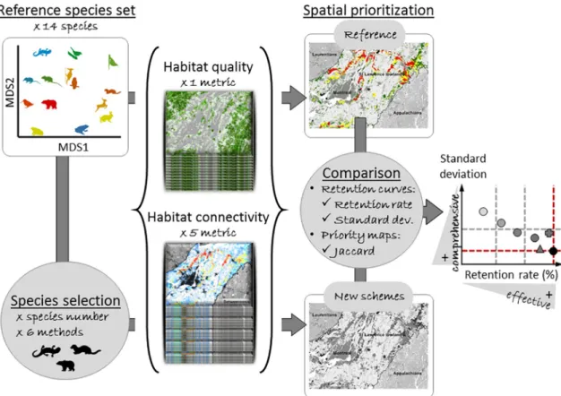
Fig. 1. General work flow. The reference spatial prioritization is obtained from one metric of habitat quality and five metrics of habitat connectivity for each of the 14

species within the reference set. These species have been selected from the forest regional species pool to reflect a diversity of habitat needs (differences in habitat requirements from Table B1 are displayed by the two axes of a non-metric multidimensional scaling analysis: MDS1 & MDS2) and movement abilities (from low: blue to high: red natal dispersal). New prioritization schemes are performed based on the requirements of subsets of species selected from the reference species set based on different species number and selection method. Schemes' performance is assessed by comparing their effectiveness (high retention rate) and comprehensiveness (low standard deviation) at retaining species-specific conservation criteria. Performance is expected to increase with species number (from low: light grey to high: black) and to change with selection methods for a given species number (displayed as different symbols). Dashed lines represent the reference values (red) and arbitrary thresholds of 80 and 90% of the reference retention rate and 120% of its standard deviation. (For interpretation of the references to color in this figure legend, the reader is referred to the web version of this article.)

Zonation iteratively discards the least valuable pixels regarding pro-vided criteria (input layers) such that the marginal loss of conservation value across the entire landscape is minimized. Here 84 criteria were used, namely 1 map of habitat quality and 5 maps of habitat con-nectivity per surrogate species (14). Final products are: 1) a priority-map, which ranks all the pixels in the landscape from lowest to highest conservation priority (Fig. B4) and 2) a set of performance curves that quantify the fraction of the total values of each criterion remaining for any percentage of the top-ranked pixels protected (Fig. B5).

We acknowledge that algorithms like Zonation select subsets of the landscape that maximize a set of static conservation values. This might be an issue regarding the spatial contingency and dynamic nature of connectivity (Gonzalez et al., 2018); a “high-value” area for habitat quality or connectivity may become “low-value” when the rest of the network changes (e.g.Rubio et al., 2015). We believe however that our choice is appropriate because: 1) by balancing a variety of multi-species and multi-metric criteria we do not focus on the most important node according to a single criteria; 2)Albert et al. (2017)showed using land use change simulations that such prioritizations could actually maintain connectivity; 3) our habitat graphs are very large (on average 4700 nodes) which prevents the use of multi-node removal optimization (~20 nodes inRubio et al., 2015); 4) inAlbert et al. (2017), simulated land-use change causes node loss ~10% of the time, but more often (~20% of the time) existing patches are fragmented or lose area. This mixed form of network erosion is likely to be common in many land use change scenarios and cannot be represented by node removal only.

To minimize biological loss, a core-area removal rule (removal rule = 1) was used; it enhances areas with maximal values of criteria and increases the importance of rare features.

To save computing time (our landscapes were represented by 27 million pixels), cells from the edges of the remaining landscape were removed first (edge removal = 1) and 10,000 cells were removed at each iteration (warp factor) (Lehtomäki and Moilanen, 2013). We did not use randomly generated edge points (add edge points = 0), but due to the diversity and the spatial heterogeneity of our conservation cri-teria, the edge removal procedure was only clearly visible for very low thresholds of priority (> 20–30% of the landscape lost), which does not affect our conclusions.

To expand upon existing protected areas, we used existing protected areas as a removal mask layer during the prioritization procedure. By artificially giving the highest conservation values to existing protected areas, surrounding cells are kept longer in the analysis, potentially leading to the identification of more compact future reserves.

All species were given equal weights. All criteria were also given equal weights (=1) (Arponen et al., 2012). We used two estimates of movement ability, so each dEC layer was given half the weight (=0.5) (Table B2). Also see Section 2.5 and Appendix A for a sensitivity analysis.

2.3. Prioritization schemes with no or fewer surrogate species

To test how the selection of surrogate species affects prioritization outcomes, we ran 43 new prioritization schemes using no surrogate species (forest habitat) or subsets of species selected from the reference species set (seeSection 2.2.1) based on a combination of 6 different concepts (single, umbrella, taxonomy, habitat diversity, movement diversity,

movement and habitat diversity) and 5 different numbers of species

(N = 1, 3, 5, 7, or 9) (Table 1). A random scheme, was also performed by removing cells randomly whatever their conservation value (re-moval rule = 5). This scheme was used as a null model to compare the outcomes of incidental representation with deliberate selection (Grantham et al., 2010). Weights were set to 0 for the criteria associated to unselected species. Unless otherwise specified, we kept the other parameters in Zonation unchanged (seeSection 2.2.3).

2.3.1. No surrogate species: habitat surrogates

In the forest habitat schemes (4), habitat and connectivity needs were defined without referring to any species in particular, i.e. based on all forested areas. This is what is classically done when little informa-tion is available on species habitat needs. To test the effect of different movement abilities on the resulting conservation priorities, we calcu-lated dEC with three different values for D50: 800 m, 4000 m, and

40,000 m, which correspond respectively to the 20%, 50%, and 90% quantiles of natal dispersal for the 14 surrogate species. Prioritization analyses were run for each of the three distances separately (weight 1 for the unique dEC layer) and for all three distances together (weight 1/ 3 for each dEC layer). Mixed prioritization combining the indirect and the species-based approaches were also performed (Appendix A).

2.3.2. Subsets of surrogate species

The single schemes (14) each accounted for only one of the species. For the schemes related to the other five concepts, subsets of N (N = 3, 5, 7, or 9) species were selected as follows: 1) umbrella: we selected species with the highest body mass (proxy for their home range size,Bowman et al., 2002); 2) taxonomy: we selected at random N/3 species among the mammals, birds, and amphibians. If N/3 contained a decimal, priority was given to mammals and birds that are more fre-quently used as surrogate species in conservation plans. This random selection was done twice to test the repeatability of this method; 3)

habitat diversity, movement diversity, or habitat & movement diversity, we

selected the most diverse subsets of species with respect to their habitat preferences and/or movement abilities. We searched across all possible subsets of N species the one maximizing the Rao quadratic entropy (Pavoine et al., 2005). Dissimilarities among species were calculated as a Gower's distance including the main habitat preferences and move-ment ability parameters from the habitat and graph models (Table B1); weights were adjusted to give equal importance to habitat and move-ment.

2.4. Comparing prioritization schemes to the reference set

The 14-species prioritization detailed inSection 2.2(Fig. B4) was used as the reference and all the prioritizations we ran inSection 2.3 were compared to it. The comparison of prioritization schemes was done in two different ways: 1) comparison of their performance curves to analyze how well and how evenly they retain the different con-servation criteria when the top priorities are protected, and 2) com-parison of the priority-rank maps to analyze the spatial congruence of conservation priorities.

Three conservation thresholds were used: 17% to follow the Aïchi biodiversity targets (CBD, 2010), and 5 and 10% as typical intermediate levels of protection. Results for 10% (respectively 5, 17%) are provided in the main text (respectively in Appendices A & C).

2.4.1. Comparison of the performance curves

To assess the performance of the different prioritization schemes we calculated two complementary metrics.

First, we calculated the retention rate, i.e. the percentage of the 84 conservation criteria retained for a given conservation threshold (5, 10, 17%). This retention rate is associated with the concepts of ‘effective-ness’ (gap between the representation target required and the one at-tained by the existing network), ‘adequacy’ (extent to which reserves fulfil their basic purpose of conserving biodiversity), and ‘representa-tiveness’ (fraction of surrogates that meet their set targets) from Kukkala and Moilanen (2013). A higher retention rate indicates a more effective prioritization scheme because it means the criteria are overall better retained. Note that we do not address the economic dimensions. Second, we calculated the standard deviation of the criteria reten-tion at the species-level. This standard deviareten-tion is associated with the concepts of ‘comprehensiveness’ (a comprehensive reserve system is

one that contains examples of many biodiversity features) and ‘com-plementarity’ (number of unrepresented species that a new area adds) (Kukkala and Moilanen, 2013). A lower standard deviation indicates a more comprehensive prioritization scheme because it means that the criteria for all species (and thus their habitat and connectivity re-quirements) are retained similarly whether they are included in the scheme or not.

Arbitrarily we classified as ‘effective and comprehensive’ schemes with retention rates within 80% and with a standard deviation within 120% of the reference schemes.

2.4.2. Comparison of priority-rank maps

To compare two priority-rank maps for a given conservation threshold (5, 10, 17%), we used the Jaccard index, which is the ratio between their intersection (both prioritization schemes agree that a given area is among the top priorities) and their union (one, the other, or both schemes agree that a given area is among the top priorities):

= > > > > Jaccard prm prm x prm x prm x prm x prm x ( 1, 2, %) 1 %_% 2 %_% 1 2 (1)

where prmi> x% is the top 5, 10, or 17% of the priority-rank map

of prioritization scheme i. This index ranges from 0 (top priorities are completely disjoint in the 2 maps) to 1 (top priorities are fully over-lapping in the 2 maps).

2.5. Sensitivity analyses

To test the robustness of our conclusions, we ran three sets of sen-sitivity analyses (Appendix A).

First, to estimate the relative contribution of each species to the prioritization results and test the robustness of the 14-species reference set, we ran 39 different schemes in which only one or two species out of fourteen were unselected.

Second, we tested the sensitivity of the conservation priorities to Zonation's main parameters with 16 different schemes (Table A1): re-moval rule (CAZ: Core-Area Zonation or ABF: Additive Benefit Function), warp factor (100, 1000 or 10,000), with and without ‘edge removal’ and ‘add edge points’, using or not protected areas as a mask, and with different weighting schemes (habitat quality: 1 and habitat connectivity: 0, 1, 4).

Third, to test the robustness of our conclusions with regard to Zonation parameterization and based on the results from the previous sensitivity analysis (seeSection 3.4), we reran the 42 prioritization schemes with species subsets (all but random, seeSection 2.3) with an ABF removal rule, and with a balanced weighting scheme (habitat quality: 1 and habitat connectivity: 1).

3. Results

3.1. Effect of species number

As species number increases, the retention rate and the Jaccard index increase while the standard deviation decreases; they all show non-linear trends and they converge asymptotically towards the values obtained with the reference set (Fig. 2). Overall, identifying priorities based on more species leads to prioritization schemes that are more effective (higher rates), more comprehensive (smaller standard devia-tion), and that are spatially more congruent with the reference set

Table 1

List of species subsets used in the prioritization schemes - Selection of species subsets among the reference species set, with increasing species numbers, and based on different methods.

Selection method Species nb. Schemes nb. Selected species or selection criteria Reference 14 1 All speciesa

Random 0 1 Cells removed randomly (no criteria accounted for)

Forest habitat 0 4 Forest habitat & connectivity layers with dispersal distance 800 m Forest habitat & connectivity layers with dispersal distance 4000 m Forest habitat & connectivity layers with dispersal distance 40,000 m

Forest habitat & connectivity layers with dispersal distances 800, 4000, and 40,000 m Single species 1 14 Habitat quality & connectivity layers for each of the 14 species separately

Umbrella 3 1 Lea, Odv, Uraa

5 1 Lea, Maa Odv, Stv, Uraa

7 1 Drp, Lea, Maa, Odv, Scm, Stv, Uraa

9 1 Bua, Drp, Lea, Maa, Odv, Scm, Sea, Stv, Uraa

Taxonomy 3 2 Bua, Drp, Leaa

Blb, Ras, Stva

5 2 Bua, Drp, Lea, Pel, Sica

Blb, Drp, Maa, Ras, Stva

7 2 Blb, Bua, Drp, Lea, Pel, Sic, Stva

Blb, Drp, Maa, Odv, Ras, Sea, Stva

9 2 Blb, Bua, Drp, Lea, Pel, Plc, Sic, Stv, Uraa

Blb, Drpi, Lea, Maa, Odv, Plc, Ras, Sea, Stva

Habitat diversity 3 1 Bua, Scm, Sica

5 1 Bua, Maa, Plc, Sic, Uraa,b

7 1 Blb, Bua, Lea, Maa, Plc, Sic, Uraa

9 1 Blb, Bua, Lea, Maa, Plc, Ras, Scm, Sic, Uraa

Movement diversity 3 1 Blb, Plc, Uraa

5 1 Blb, Maa, Plc, Ras, Uraa

7 1 Blb, Maa, Plc, Ras, Sea, Stv, Uraa

9 1 Blb, Maa, Plc, Ras, Scm, Sea, Sic, Stv, Uraa

Habitat and movement diversity 3 1 Maa, Plc, Uraa

5 1 Bua, Maa, Plc, Sic, Uraa,b

7 1 Maa, Plc, Ras, Scm, Sea, Sic, Uraa

9 1 Blb, Bua, Maa, Plc, Ras, Scm, Sic, Stv, Uraa

Abbreviations: nb.: number; Blb: Blarina brevicauda; Bua: Bufo americanus; Drp: Dryocopus pileatus; Lea: Lepus americanus; Maa: Martes americana; Odv: Odocoileus virginianus; Pel: Peromyscus leucopus; Plc: Plethodon cinereus; Ras: Rana sylvatica; Scm: Scolopax minor; Sea: Seiurus aurocapilla; Sic: Sitta canadensis; Stv: Strix varia; Ura Ursus americanus.

a _{Habitat quality & connectivity layers for the given species (details in Table B2).} b _{Same subsets.}

(higher jaccard index,Fig. 2). Results are very similar with 5% and 17% thresholds (Fig. A5).

3.2. Effect of species selection

Beyond species number, the concepts used to select species also lead to a great variability in the performance of the prioritization schemes. The best performing schemes are the three diversity-based schemes, the

habitat diversity scheme performing slightly less well and the movement diversity scheme performing slightly better than the others (Fig. 2). The three diversity-based schemes lead to priority-rank maps that are fairly similar to the reference set. The taxonomy scheme also leads to effective and comprehensive schemes on average, but with little repeatability among the two runs. The umbrella schemes are not comprehensive (high standard deviations, 125–160% of reference) though they are not par-ticularly ineffective (Fig. 2). Both taxonomy and umbrella schemes lead

to priority-rank maps that are moderately similar to the reference set. All the single schemes - with the exception of Dryocopus pileatus – per-form poorly and they all lead to priority-rank maps that strongly differ from the reference (Fig. 2).

Forest habitat schemes – whatever the movement ability – perform

less well (less effective and less comprehensive) than the other schemes and lead to priority-rank maps that strongly differ from the reference map. However, they perform better and lead to priority-rank maps more similar to the reference, than single schemes (Fig. 2). Interestingly, the forest habitat schemes are more comprehensive (lower standard deviation) than the reference. Mixing ‘Forest habitat’ and species-spe-cific criteria for 3, 5, or 7 species (movement diversity or habitat and

movement diversity) within schemes does not improve effectiveness

(Appendix C).

Overall, selection procedure plays a crucial role as some 3-species schemes are more effective and comprehensive than some 9-species

Fig. 2. Comparison of the prioritization schemes' performance (top 10% priorities conserved) – Effectiveness (high retention rate, top) and comprehensiveness (low

standard deviation, middle) at retaining species-specific conservation criteria, and spatial agreement with the reference scheme (high Jaccard index, bottom) are given as a function of species number (left column) and selection method (right column). Symbols represent the different concepts used for species selection. Dashed lines represent the reference values (red), the random scheme (black), the arbitrary thresholds of 80 and 90% of the reference retention rate and 120% of its standard deviation (grey). The box-and-whisker plots display the median (central bar), the first and third quartiles (Q1 and Q3, box envelope), whiskers show the max (respectively min) between max (respectively min) value and Q3 + 1.5(Q3-Q1) (respectively Q1 − 1.5 (Q3-Q1)), dots are values beyond the whiskers. (For inter-pretation of the references to color in this figure legend, the reader is referred to the web version of this article.)

schemes. The schemes based on diversity are globally effective and comprehensive, in particular for 5 species or more (Fig. 2).

Results are fairly similar with 5% and 17% thresholds (Appendix C).

3.3. Spatial agreement among prioritizations

When we overlap the top 10% priorities identified by 43 of our prioritization schemes (reference, forest habitat, and 1–9 species schemes) a series of large stepping-stone patches emerge to the north, which delineate the easiest paths to traverse the Lowlands between the Appalachian and Laurentian Mountains (Fig. 3a). Areas of disagreement are mainly smaller and scattered habitat patches that are found essen-tially to the northeast and southwest of the lowlands. Increasing the conservation threshold (from 5%, to 10 and 17%) exacerbates the im-portance of the series of stepping stone patches and increases the agreement among schemes (Fig. A6).

The 5-species movement diversity scheme (hereafter ‘5sp-disp’) pre-sents a trade-off between parsimony (few species) and a high perfor-mance (effectiveness and comprehensiveness). ‘5sp-disp’ identifies the same series of stepping-stone forest patches to the north as the reference (Fig. 3b). Disagreement areas are scattered to the south and along the series of stepping-stone patches.

3.4. Sensitivity analyses

First, not including only one or two species from the reference set (12- and 13-species schemes) leads to effective and comprehensive schemes; some of these schemes are even marginally more effective (higher retention rate) and comprehensive (lower standard deviation) than the reference set (Fig. A1). They also lead to priority-rank maps very similar to the reference (Jaccard: 0.76–0.99).

Second, we found that two Zonation's parameters mainly influence prioritization outcomes and may modify findings based on the selection of surrogate species (Table A2): 1) changing the relative weights at-tributed to conservation criteria; and 2) using an Additive Benefit

Function (ABF) instead of a Core-Area Zonation (CAZ) removal rule. Third, species number (Section 2.1) and species selection (Section 2.2) results remain robust when switching the removal rule from CAZ to ABF, or when altering the weighting choices (Figs. A2 & A3). ABF schemes lead to higher retention rates and lower standard deviations for a given scheme, but the highest values of each criterion are better conserved with CAZ (Fig. A4). This is expected given that ABF favors criteria-rich areas while CAZ focuses on the highest-quality locations for each criterion (Lehtomäki and Moilanen, 2013). Giving more weight to habitat quality leads to lower retention rates and higher standard deviations, due to a lower retention of connectivity layers. The relative performance of the diversity-based schemes changes slightly; the two schemes including habitat diversity become slightly improved com-pared to the movement diversity scheme.

4. Discussion

Here we compared the performance and spatial agreement of dif-ferent prioritization schemes obtained with systematically-selected sets of surrogate species. Our 14-species set was a relatively robust reference given the asymptotic convergence to its values and the highly similar schemes (performance and maps) obtained when removing only 1 or 2 species. Our results also remain robust to the other major sources of uncertainty found behind spatial conservation prioritization based on habitat quality and connectivity (e.g., removal rule, weights). Therefore, we will discuss three main points that may help build ef-fective sets of surrogate species for connectivity conservation.

4.1. Species are more effective surrogates than habitat

We found that basing conservation priorities on the connectivity of forest habitat is globally less effective than doing the same thing with few surrogate species (≥3), but still more effective than doing so with a single surrogate species. It also leads to priorities that are spatially more different from the reference set. This extends previous findings from

Fig. 3. Spatial agreement among conservation priorities (top 10%) obtained with prioritization schemes based on contrasting numbers and selections of species - a)

priorities from all 43 prioritization schemes (1–9 species schemes, Forest habitat, and reference) following a yellow (few) to red gradient (most); b) priorities from the 5-species movement diversity scheme (5sp-div.mvt.: blue), the 14-species reference scheme (14sp: yellow) or both simultaneously (green). The grey shades display the underlying simplified land cover (both panels).

Krosby et al. (2015)who found that conservation priorities based on habitat naturalness were more different from the reference (in their case 16-species scheme) than the ones obtained with > 3–4 randomly selected species. However, in our case forest habitat priorities balance the requirements of the different species well (low standard deviation), whileKrosby et al. (2015)found that naturalness-based networks better agree with corridor networks of far-dispersing species. Interestingly, we found that including different movement distances in the forest habitat prioritization did not lead to any significant change, which seems contradictory with the necessity to encompass different scales of con-nectivity. As it accounts for all forested areas with no specific focus on species' needs, the forest habitat scheme does not capture the most im-portant areas for each species, whatever the distance considered. Con-trary to other studies (e.g.Di Minin and Moilanen, 2014), we also found little support for a mixed approach. Indeed, when combining habitat-based criteria with species-habitat-based criteria, the results were always very similar to the equivalent species-based schemes.

4.2. A moderate number of species might be sufficient

Overall, our results are in agreement with previous studies, and a greater number of species leads to more effective prioritization schemes that also match the reference priority-rank map better (Roberge and Angelstam, 2004). However, expanding on the results fromKrosby et al. (2015, spatial overlap only)and contrary toLindenmayer et al. (2002), we show that a relatively modest number of surrogate species (N ≥ 5) captured relatively well the needs of the fourteen species and led to priority maps that where fairly similar (N ≥ 7) to the reference set. Interestingly, the rate with which the spatial priorities converge (Fig. 2) is lower than in Krosby et al. (2015), probably because here the 14 species were selected specifically to maximize differences in habitat needs and movement abilities. The rate with which the spatial priorities converge is also much lower than the one with which retention rate saturates (Fig. 2). This suggests that in our case different spatial con-servation solutions may equally meet concon-servation criteria.

Our results also indicate that increasing the number of surrogate species beyond 7–9 leads to decreasing returns; each additional species means more work but a small increase in the schemes' performance. In our case, increasing species number beyond 12 is also marginally counter-productive regarding the overall performance because spatial priorities are highly similar and the schemes' performance marginally better than with 14 species. The fact that a schemes' performance sa-turates so quickly when increasing species number is encouraging be-cause it suggests that adding a 15th forest species with subtly different habitat needs or movement ability would not modify greatly the schemes or their performances. In addition, given that the reference species set has already been selected to reflect contrasting habitat needs and movement abilities, it is expected it also reflects the needs of the many other vertebrate species within the regional species pool (see Fig. M1.1 in Albert et al., 2017). A major limitation of this dataset is, however, that – like many sets of surrogate species – it contains only vertebrates due to a lack of good data for other taxa from the study area; better data is required to assess how effective our schemes are for plants and insects, for instance. In addition, we focused here only on forest (and treed-wetland) biodiversity, making a full regional assess-ment of regional connectivity for all ecosystem types (open areas, aquatic habitats) would require additional surrogates and would lead to stronger conservation trade-offs (Breckheimer et al., 2014).

4.3. ‘How’ is as important as ‘how many’

The number of surrogate species is not the only factor determining a schemes' performance and the associated priorities. In contrast to the prediction made byLindenmayer et al. (2002)that ‘no scheme captured more species [needs] […] than species selected at random’, schemes can vary greatly depending on how surrogate species have been

selected. In agreement with the ecoprofiles concept (Vos et al., 2001; Wiens et al., 2008), selecting a few surrogates based on the diversity of needs of the species pool may be the best compromise to build a high-performing conservation scheme. The three diversity-based schemes were indeed the best performing. The movement diversity (respectively

habitat diversity) scheme performed marginally better (respectively

worse) than the other two under the reference parameterization; but these marginal differences were not robust to a modification of the weighting scheme. Schemes favoring habitat quality (respectively connectivity) may perform better when selecting species based on their diversity of habitat needs (respectively movement abilities, Silvano et al., 2017,Lechner et al., 2016). The fact that the habitat and

move-ment diversity scheme did not perform better than the other two, may be

because the reference set was already chosen to reflect the diversity of habitat needs and movement abilities of the regional pool.

Two commonly used methods for species selection in applied con-servation (taxonomy and umbrella), performed poorly and led to priority-rank maps that strongly differed from the reference maps. In particular, the taxonomy schemes led to results with low repeatability. Selecting species from different taxa is expected to enlarge the diversity of needs covered (Di Minin and Moilanen, 2014) but our results ques-tion the reliability of this often-used concept to properly select species subsets. In agreement with previous studies, we also found the ‘area-demanding’ umbrella species perform very poorly and do not cover the needs of a diversity of species (Breckheimer et al., 2014). It has been thought for a long time that area-demanding species should encompass the needs of less-area demanding ones, butCushman et al. (2013)found habitat specialists with limited movement ability to be weak indicators of others, and to be weakly indicated by others. Here we obtained high standard deviations for criteria retention among species with these schemes, meaning that some species' needs (those with small body mass) are poorly represented. If the poor dispersers (e.g. salamander) may not actually need connectivity at broader scales, their habitat needs – along with the needs of species sharing these habitats – must still be preserved. From our results, Dryocopus pileatus (classically an ‘indicator species’ for old forests) and Strix varia (owls are classical umbrella species) could still appear as good ‘umbrella species’ as they lead to relatively effective and comprehensive schemes when conser-ving 10% of the landscape. However, given the low reliability of this approach (performances are bad for these two species with a 5% con-servation threshold, and for all the other single-species schemes), we believe an umbrella-type selection of species should be avoided.

5. Conclusion: how to select surrogate species for connectivity conservation?

We close with four points that may help the future selection of surrogate species sets for connectivity conservation. First, species se-lection should match the conservation objectives. When dealing with connectivity conservation, the ecoprofile approach seems effective (Vos et al., 2001), i.e. species are selected based on characteristics related to their vulnerability to habitat fragmentation, habitat preferences and movement abilities. A few species (5–7) selected with this flexible ap-proach may be the best option to successfully prioritize a habitat net-work (for one type of ecosystem) and coincide conservation objectives with data availability and stakeholder objectives (Opdam et al., 2008; Wiens et al., 2008). Second, when too little is known about the local biodiversity, or and when resources are insufficient to conduct a proper surrogate species approach, an indirect approach may safely replace a species-based approach, though it may lead to spatial conservation priorities that do not align with the most important areas in terms of species-specific habitat quality and connectivity. This should be pre-ferred to an umbrella, or taxonomy-based, selection of surrogate species (Lehtomäki et al., 2009; Krosby et al., 2015). Third, ideally species selection should be made more explicit in projects focused on con-nectivity conservation; the performance of different selection methods

can only be assessed when selection methods are more systematically described. Fourth, future studies on this topic need to go further than a simple examination of the spatial match among conservation solutions (e.g.Krosby et al., 2015;Breckheimer et al., 2014) and actually assess how satisfactory the solutions are, for instance with measures of ef-fectiveness or comprehensiveness, at representing the habitat and functional connectivity needs of a diversity of species (Grantham et al., 2010). Assessing the cost-effectiveness of these solutions would also foster the implementation phase of a planned ecological network (Dilkina et al., 2017).

Supplementary data to this article can be found online athttps:// doi.org/10.1016/j.biocon.2018.09.028.

Acknowledgments

This research was funded by the Mediterranean Institute of Biodiversity and Ecology (PPM team). Computations were performed using the computing platform “Cluster de calcul intensif HPC” of the OSU Institut Pythéas (Aix-Marseille Université, INSU-CNRS). We thank M. Libes and C. Yohia, from the Service Informatique de Pythéas (SIP), for their technical assistance. We thank A. Millon, B. Rayfield, and M. Dumitru for their help and comments on earlier phases of this work. This work contributes to the Agence Nationale de la Recherche (ANR) (number ANR-11-LABX-0061) funded by the French government through the A∗MIDEX project (number ANR-11-IDEX-0001-02). AG is supported by the Liber Ero Chair in Biodiversity Conservation.

References

Adriaensen, F., Chardon, J.P., De Blust, G., Swinnen, E., Villalba, S., Gulinck, H., Matthysen, E., 2003. The application of ‘least-cost’ modelling as a functional land-scape model. Landsc. Urban Plan. 64, 233–247.

Albert, C.H., Rayfield, B., Dumitru, M., Gonzalez, A., 2017. Applying network theory to prioritize multi-species habitat networks that are robust to climate and land-use change. Conserv. Biol. 31 (6), 1383–1396.

Anderson, M.G., Ferree, C.E., 2010. Conserving the stage: climate change and the geo-physical underpinnings of species diversity. PLoS One 5, e11554.

Arponen, A., Lehtomäki, J., Leppänen, J., Tomppo, E., Moilanen, A., 2012. Effects of connectivity and spatial resolution of analyses on conservation prioritization across large extents. Conserv. Biol. 26 (2), 294–304.

Bowman, J., Jaeger, J.A.,.G., Fahrig, L., 2002. Dispersal distance of mammals is pro-portional to home range size. Ecology 83 (7), 2049–2055.

Breckheimer, I., Haddad, N.M., Morris, W.,.F., Trainor, A.M., Fields, W.R., Jobe, R.T., Hudgens, B.R., Moody, A., Walters, J.R., 2014. Defining and evaluating the umbrella species concept for conserving and restoring landscape connectivity. Conserv. Biol. 00 (0), 1–10.

Caro, T.M.G., O'Doherty, G., 1999. On the use of surrogate species in conservation biology. Conserv. Biol. 13 (4), 805–814.

Carroll, C., Noss, R.F., Paquet, P.,.C., 2001. Carnivores as focal species for conservation planning in the rocky mountain region. Ecol. Appl. 11 (4), 961–980.

Convention on Biological Diversity (CBD), 2010. COP-10 Decision X/2, ed. C. Secretariat, Montreal.

Cushman, S.A., Landguth, E.L., 2012. Multi-taxa population connectivity in the Northern Rocky Mountains. Ecol. Model. 231, 101–112.

Cushman, S.A., Landguth, E.L., Flather, C.H., 2013. Evaluating population connectivity for species of conservation concern in the American Great Plains. Biodivers. Conserv. 22 (11), 2583–2605.

Di Minin, E., Moilanen, A., 2014. Improving the surrogacy effectiveness of charismatic megafauna with well-surveyed taxonomic groups and habitat types. J. Appl. Ecol. 51 (2), 281–288.

Dilkina, B., Houtman, R., Gomes, C.P., Montgomery, C.A., McKelvey, K.S., Kendall, K., ... Schwartz, M.K., 2017. Trade-offs and efficiencies in optimal budget-constrained multispecies corridor networks. Conserv. Biol. 31 (1), 192–202.

Fall, A., Fall, J., 2001. A domain-specific language for models of landscape dynamics. Ecol. Model. 141, 1–18.

Freeman, L.C., 1979. Centrality in social networks conceptual clarification. Soc. Networks 1, 215–239.

Gonzalez, A., Thompson, P., Loreau, M., 2018. Spatial ecological networks: planning for sustainability in the long-term. Curr. Opin. Environ. Sustain. 29, 187–197.

Grantham, H.S., Pressey, R.L., Wells, J.A., Beattie, A.J., 2010. Effectiveness of biodiversity surrogates for conservation planning: different measures of effectiveness. PLoS One 5 (7).

Heller, N.E., Zavaleta, E.S., 2009. Biodiversity management in the face of climate change: a review of 22 years of recommendations. Biol. Conserv. 142, 14–32.

Henle, K., Davies, K.F., Kleyer, M., Margules, C., Settele, J., 2004. Predictors of species sensitivity to fragmentation. Biodivers. Conserv. 13, 207–251.

Krosby, M., Breckheimer, I., Pierce, D.J., Singleton, P.H., Hall, S.A., Halupka, K.C., Gaines, W.L., Long, R.A., McRae, B.H., Cosentino, B.L., Schuett-Hames, J.P., 2015. Focal species and landscape “naturalness” corridor models offer complementarity approaches for connectivity conservation planning. Landsc. Ecol. 30, 2121–2132.

Kukkala, A.S., Moilanen, A., 2013. Core concepts of spatial prioritization in systematic conservation planning. Biol. Rev. 88 (2), 443–464.

Lambeck, R., 1997. Focal species: a multiple-species umbrella for nature conservation. Conserv. Biol. 11 (4), 849–856.

Lechner, A.M., Sprod, D., Carter, O., Lefroy, E.C., 2016. Characterising landscape con-nectivity for conservation planning using a dispersal guild approach. Landsc. Ecol. 32 (1), 1–15.

Lehtomäki, J., Moilanen, A., 2013. Methods and workflow for spatial conservation prioritization using Zonation. Environ. Model. Softw. 47, 128–137.

Lehtomäki, J., Tomppo, E., Kuokkanen, P., Hanski, I., Moilanen, A., 2009. Applying spatial conservation prioritization software and high-resolution GIS data to a na-tional-scale study in forest conservation. For. Ecol. Manag. 258 (11), 2439–2449.

Lindenmayer, D.B., Manning, A.D., Smith, P.L., Possingham, H.P., Fischer, J., Olivier, I., McCarthy, M.A., 2002. The focal-species approach and landscape restoration: a cri-tique. Soc. Conserv. Biol. 16 (2), 338–345.

Magris, R.A., Reml, E.A., Pressey, R.L., Weeks, R., 2015. Integrating multiple species connectivity and habitat quality into conservation planning for coral reefs. Ecography 39, 649–664.

McRae, B.H., Dickson, B.G., Keitt, T.H., Shah, V.B., 2008. Using circuit theory to model connectivity in ecology evolution and conservation. Ecology 89 (10), 2712–2724.

Mitchell, M.G.E., et al., 2015. The Montérégie Connection Project: linking landscapes, biodiversity, and ecosystem services to improve decision-making. Ecol. Soc. 20 (art. 15).

Moilanen, A., Pouzols, F.M., Meller, L., Arponen, A., Leppänen, J., Kujala, H., 2014. Spatial Conservation Planning Methods and Software: ZONATION. Version 4. User Manual.

Olds, A.D., Connolly, R.M., Pitt, K.A., Maxwell, P.S., Aswani, S., Albert, S., 2014. Incorporating surrogate species and seascape connectivity to improve marine con-servation outcomes. Conserv. Biol. 28 (4), 982–991.

Opdam, P., Pouwels, R., Van Rooiji, S., Steingröver, E., Vos, C.C., 2008. Setting biodi-versity targets in participatory regional planning: introducing ecoprofiles. Ecol. Soc. 13 (1), 20.

Pavoine, S., Ollier, S., Pontier, D., 2005. Measuring diversity from dissimilarities with Rao's quadratic entropy: are any dissimilarities suitable? Theor. Popul. Biol. 67 (4), 231–239.

Pelletier, D., Clark, M., Anderson, M.G., Rayfield, B., Wulder, M.A., Cardille, J.A., 2014. Applying circuit theory for corridor expansion and management at regional scales: tiling, pinch points, and omnidirectional connectivity. PLoS One 9 (1), 1–11.

Roberge, J.M., Angelstam, P., 2004. Usefulness of the umbrella species concept as a conservation tool. Conserv. Biol. 18 (1), 76–85.

Rubio, L., Bodin, O., Brotons, L., Saura, S., 2015. Connectivity conservation priorities for individual patches evaluated in the present landscape: how durable and effective are they in the long term? Ecography 38, 001–010.

Saura, S., Estreguil, C., Mouton, C., Rodríguez-Freire, M., 2011. Network analysis to as-sess landscape connectivity trends: application to European forests (1990–2000). Ecol. Indic. 11 (2), 407–416.

Silvano, A.L., Guyer, C., Steury, T.D., Grand, J.B., 2017. Selecting focal species as sur-rogates for imperiled species using relative sensitivities derived from occupancy analysis. Ecol. Indic. 73, 302–311.

Taylor, P.D., Fahrig, L., Henein, K., Merriam, G., 1993. Connectivity is a vital element of landscape structure. Oikos 68, 571–573.

Théau, J., Bernier, A., Fournier, R.A., 2015. An evaluation framework based on sustain-ability-related indicators for the comparison of conceptual approaches for ecological networks. Ecol. Indic. 52, 444–457.

Vos, C.C., Verboom, J., Opdam, P., Braak, C., 2001. Toward ecologically scaled landscape indices. Am. Nat. 183 (1), 24–41.

Watson, J., Freudenberger, D., Paull, D., 2001. An assessment of the focal-species ap-proach for conserving birds in variegated landscapes in southeastern Australia. Conserv. Biol. 15 (5), 1364–1373.

Wiens, J.A., Hayward, G.D., Holthausen, R.S., Wisdom, M.J., 2008. Using surrogate species and groups for conservation planning and management. Bioscience 58 (3), 241–252.