Data and text mining
Advance Access publication January 26, 2010Predicting biodegradation products and pathways: a hybrid
knowledge- and machine learning-based approach
Jörg Wicker
1, Kathrin Fenner
2,3, Lynda Ellis
4, Larry Wackett
5and Stefan Kramer
1,∗ 1Institut für Informatik/I12, Technische Universität München, Boltzmannstr. 3, D-85748 Garching b. München, Germany,2Eawag, Swiss Federal Institute for Aquatic Science and Technology, CH-8600 Dübendorf,3Institute of Biogeochemistry and Pollutant Dynamics (IBP), ETH Zurich, CH-8092 Zürich, Switzerland,4Department of Laboratory Medicine and Pathology, University of Minnesota, Minneapolis, MN 55455 and5Department of Biochemistry, Molecular Biology and Biophysics, University of Minnesota, St. Paul, MN 55108, USA Associate Editor: Jonathan WrenABSTRACT
Motivation: Current methods for the prediction of biodegradation products and pathways of organic environmental pollutants either do not take into account domain knowledge or do not provide probability estimates. In this article, we propose a hybrid knowledge- and machine learning-based approach to overcome these limitations in the context of the University of Minnesota Pathway Prediction System (UM-PPS). The proposed solution performs relative reasoning in a machine learning framework, and obtains one probability estimate for each biotransformation rule of the system. As the application of a rule then depends on a threshold for the probability estimate, the trade-off between recall (sensitivity) and precision (selectivity) can be addressed and leveraged in practice.
Results: Results from leave-one-out cross-validation show that a recall and precision of ∼0.8 can be achieved for a subset of 13 transformation rules. Therefore, it is possible to optimize precision without compromising recall. We are currently integrating the results into an experimental version of the UM-PPS server.
Availability: The program is freely available on the web at http://wwwkramer.in.tum.de/research/applications/ biodegradation/data.
Contact: [email protected]
Received on August 11, 2009; revised on December 30, 2009; accepted on January 17, 2010
1 INTRODUCTION
In silico methods to predict products and pathways of microbial
biotransformations of chemical substances are increasingly sought due to rapidly growing data requirements for regulatory chemical risk assessment at the European (cf. REACH) and global level. Existing methods for the prediction of biotransformation products and pathways can be categorized as either knowledge- or machine learning-based approaches. Each of the two approaches has its strengths and weaknesses. Knowledge-based approaches, such as METEOR for the prediction of mammalian metabolism (Greene
et al., 1999) or the University of Minnesota Pathway Prediction
∗To whom correspondence should be addressed.
System (UM-PPS) for microbial biodegradation (Hou et al., 2004) take into account expert knowledge on the basis of sets of transformation rules. However, they run the risk of including potentially overly general, incomplete or inconsistent rules. In contrast, machine learning approaches produce accurate probability estimates on the basis of empirical data, but often lack the ability to incorporate prior domain knowledge. Also, recent machine learning approaches for biotransformation prediction only predict quite general classes [e.g. whether a compound plays a role in central metabolism (Gomez et al., 2007) or whether it is the substrate of some broad reaction class, e.g. oxidoreductase-catalyzed reactions (Mu et al., 2006)].
The goal of this article is to combine the two approaches: we assume a given set of biotransformation rules and learn the probability of transformation products proposed by the rules from known, experimentally elucidated biodegradation pathways. Only two comparable systems exist so far: META (Klopman et al., 1997) that is similar in spirit, but uses a less-advanced problem formulation and machine learning approach than the one presented here, and CATABOL (Dimitrov et al., 2007), the only rule-based method explicitly aiming for probability estimates. However, the CATABOL system works with a fixed pathway structure for training, which is different from the approach presented here working on the basis of individual rules (for a detailed discussion, see Section 6).
Rule-based systems, such as UM-PPS, work on the basis of rules that are generalizations and abstractions of known reactions, in the case of UM-PPS, its underlying Biocatalysis/Biodegradation Database (UM-BBD; Ellis et al., 2006). UM-BBD is a manually curated compilation of over 200, experimentally elucidated microbial biotransformation pathways, encompassing enzymatic reactions for roughly 1000 parent compounds and intermediates. If certain functional groups of a query substrate match with any of the biotransformation rules in UM-PPS, then its structure is transformed into one or several products according to the rule(s). These rules are typically fairly general, either to cover all known reactions, or because there is not enough information known to restrict them. As a consequence, UM-PPS produces a large number of possible reaction products, especially when used to predict several subsequent generations of transformation products. This combinatorial explosion is a phenomenon also known from other rule-based systems and approaches. It is particularly aggravated for the structurally more complex contaminants of current concern,
e.g. pesticides, biocides or pharmaceuticals. Potential users of such a system such as environmental microbiologists, risk assessors and analytical chemists are overwhelmed by the number of possible products, and find it hard to identify the most plausible products.
In an effort to restrict combinatorial explosion, some of the knowledge-based approaches to metabolic prediction employ what is called relative reasoning (Button et al., 2003). In relative reasoning, the possibility to apply a rule depends on the presence of other applicable rules. Practically, this requires additional rules for the prioritization of rules and the resolution of conflicts. These meta-rules, or relative reasoning rules, express that some reactions take priority over others, and vice versa, and that some reactions only occur if others are not possible. Relative reasoning rules have recently been derived automatically for the set of UM-PPS biotransformation rules and have been successfully implemented into the working UM-PPS (Fenner et al., 2008). However, although reductions in the number of predicted products in one prediction step of∼20% were achieved, the selectivity (precision) of UM-PPS still remained rather low, at∼16–18%. Thus, the question remains how, when a set of rules applied to the structure of a given substrate, we can further refine the process of selecting and accepting those rules that most likely lead to observed products.
In this article, we propose a solution that transfers the idea of relative reasoning to a machine learning setting, to further improve the system’s selectivity (precision). Rule probabilities are to be estimated such that they depend not only on all other rules that are applicable, but also on the structure of the substrate. The priorities are learned statistically from data on known biodegradation pathways. In our solution, one classifier is learned for each rule, generalizing over the molecular substructures of the substrate and the ‘activation patterns’ of the rules as given by the set of all other rules that are triggered by the same substrate.
Given the availability of such probabilistic classifiers, the decision to accept a product or not can be made dependent on a probability threshold: the application of individual rules can be tuned such that only transformations with a probability above a certain threshold are accepted. In this way, one can also control the generality of whole rule sets and the overall number of products. Thus, it is easy to address the fundamental trade-off between the completeness and the accuracy of predictions. In technical terms, we can analyze the performance of both individual rules and the whole system in recall–precision space, and visualize their performance in 2D plots. Moreover, it is possible to explicitly choose a suitable point in recall– precision space by setting the probability threshold for accepting a rule to a certain level.
This article is organized as follows: In Section 2, we explain the method for learning classifiers to restrict the scope of transformation rules. Section 3 presents the data that were used as the basis of our study and some implementation details. In Section 4, the performance measures used to evaluate the results of our experiments are presented and finally, in Section 5, the results themselves are discussed.
2 METHOD
To illustrate the problem and the proposed solution, we start with an example shown in Figure 1a: given a new compound cnew, several rules of the UM-PPS are applicable and suggest possible transformation products. In
the example, a subset of rules r1,r2,r5, etc., triggers for the given input structure. In the illustration, triggering rules are indicated by solid arrows, rules not triggering by dashed arrows. As mentioned above, the problem is that the rules of the system are overly general, i.e. they suggest a wide range of possible products, many of them false positives. To restrict the number of possible products, it would be desirable to score the proposed transformations by estimated probabilities. In this way, it would also be possible to tune the number of products depending on a user-defined threshold: If the estimated probability of a transformation exceeds a threshold, it is accepted, otherwise it is discarded. The probability for each rule riis estimated by a corresponding
function fi. Function fi tells us how likely a transformation suggested by
rule riis, depending on the structure of the input compound and all other
triggering rules. This is illustrated in Figure 1b: function f1 estimates that the probability of obtaining a correct product from applying r1to substrate cnew is 0.6, given the molecular structure of cnew and the other rules applicable (r2,r5,...,r179). The dependency of the decision on all other transformation options reflects the fact that, under certain conditions, one reaction should be given priority over another. If the cut-off was set to 0.5 in the example, we would only accept the transformations proposed by r1 and r5.
The problem is of course to derive suitable probability scores. In this article, the solution is based on a training set of examples and machine learning. In Figure 1c, a sample of three compounds from a hypothetical training database is shown. For the three training compounds, we assume that we not only know which rules are applicable, but also which rule applications lead to observed products. In the figure, the observed transformation products are indicated by a check mark, whereas the spurious products are indicated by a cross. Given this information, it is possible to learn under which conditions the suggested product of a transformation rule can actually be observed. As a classifier is only needed when a rule triggers, the training set for a rule also includes only those compounds for which the rule suggests a product. Figure 1d shows two training sets constructed from the three training compounds c1–c3, one for rule r1(upper table) and one for rule r2 (lower table). The first group of features (s1,...,sm) is a fingerprint-based
representation of the structure of the input compound. The second group of features (all r1,...,r179 except the rule for which the classifier is built) indicates which other rules are applicable to the compound: a feature is set to +1, if the corresponding rule fires, and 0, otherwise. As explained above, the training set for f1does not contain an entry for c2, because rule r1is not applicable to that compound. Similarly, c1is not listed in the training set for f2, because rule r2cannot be applied. Also note that c3is a positive example for f1, whereas it is a negative example for f2. Given such training sets, any machine learning algorithm for classification can be applied to induce a mapping from the structural and rule descriptors to the target variable, i.e. whether a rule generates an observed product.
To be more precise (amongst others, to enable reproducibility), we have to introduce some notation: in the following, C denotes the set of compounds ci, and R the set of rules rj. Then triggers(rj,ci) is a predicate indicating
whether rjtriggers on compound ci. Moreover, observed(rj,ci) is a predicate
indicating that rule rjfires and provides an observed degradation product.
For instance, we have the following list of facts for c1and c2, and r1to r3 from Figure 1c: triggers(r1,c1). triggers(r3,c1). observed(r3,c1). triggers(r5,c1). observed(r5,c1). triggers(r2,c2). observed(r2,c2). triggers(r4,c2).
Finally, S denotes the set of molecular substructures sl, and predicate
occurs(sl,ci) checks the occurrence of a substructure slin a compound ci.
To prepare for training, we need two transformation operators, one for the construction of individual examples, and one for the construction of whole
(a)
(b)
(c)
(d)
Fig. 1. (a) Indication of the rules applicable to an input compound cnewby solid arrows. (b) Illustration of the use of one classifier for each rule to determine the probability of obtaining a proper product, depending on the structure and other applicable rules. (c and d) Examples for the construction of two training sets, one for f1(upper table) and other for f2(lower table).
training sets. The first one,τinstance, is defined as follows: τinstance(ci,k)= xi such that
xi,j = occurs(sj,ci) for
1≤ j ≤ |S|∧
xi,j = triggers(rj−|S|,ci) for
|S|<j ≤|S|+k −1∧ xi,j = triggers(rj−|S|+1,ci) for
|S|+k −1<j ≤|R|+|S|−1
This means that operator τinstance(ci,k) constructs the description of an
individual example without its class information. It takes a compound ci
and constructs a feature vector (see the example above), taking into account substructures and applicable rules. Parameter k is used to exclude the information for the k-th rule, which is convenient for our purposes, because it constitutes the target for training. Making use ofτinstance(ci,k), we are ready
to define a transformation operator generating a training or test set for rule k from a given set of compounds C:τsettakes a compound cifrom C and
checks whether rule k triggers. Only if this is the case, a training example (xi,yi) is constructed: τset(C,k)={(xi,yi)|ci∈C∧ triggers(rk,ci)∧ xi=τinstance(ci,k)∧ yi=1if observed(rk,ci), yi=0 otherwise}
In the above example,τset({c1,c2,c3,...,c718},1) gives us the training set for classifier f1shown in the upper table of Figure 1d,τset({c1,c2,c3,...,c718},2) gives us the training set for f2 in the lower table. A training procedure
Algorithm 1 Pseudocode for training and testing classifiers for
biotransformation rules
% training one classifier per rule for all rule rkdo
Dk
Trg:=τset(CTrg,k)
fk:=train(DkTrg)
end for
% testing for a new test compound cnew
% the cut-off for acceptance is given by parameterθ for all rule rkdo
if triggers(rk,cnew) then
if fk(τinstance(cnew,k))>θ then classify as “product of k” else
classify as “no product of k” end if
end if end for
train returns the classifiers needed for the restriction of the rules based on such training sets. As already indicated above, classifiers are represented as functions fjreturning class probability estimates for given examples.
Given those preliminaries, we can explain how training and testing is performed and how it is embedded into the working system (see Algorithm 1 for the pseudocode). In the training phase, a classifier is trained for each rule in turn. In the testing phase, we first obtain a list of rules applicable to each test compound using the UM-PPS. If a rule triggers, we apply the rule’s classifier to the instance, where information from the molecular structure and all competing rules is taken into account to obtain a probability estimate. If this estimate exceeds a thresholdθ, the product suggested by rule rk is
3 DATA AND IMPLEMENTATION
It is possible to validate the above procedure by running a cross-validation over the compounds of the UM-BBD database. This can be optimized considerably, if the predicates triggered, observed and
occurs are precomputed once for all compounds and stored for
later use. In our implementation, we precomputed a|C|×|R| table
indicating the rules’ behavior on the UM-BBD compounds: the value +1 of an entry encodes that a rule is triggered and produces an observed product, 0 encodes that a rule is triggered but the product is not observed, and−1 encodes that the rule is not triggered for a given compound. Simple database and arithmetic operations can then be applied to extract training and test sets, e.g. for (leave-one-out) cross-validation. Additionally, we learned the classifiers on the complete dataset and tested our approach on an external validation set of 25 xenobiotics (pesticides), which was also used in previous work (Fenner et al., 2008).1 Pesticide biodegradation data is the
largest cohesive dataset available, because these compounds are made to be put into the environment and are among the most heavily regulated class of chemicals.
The matrix encoding described above was applied to the UM-BBD/UM-PPS from July 24, 2007, containing 1084 compounds and 204 biotransformation rules (btrules). Of these, 366 compounds not triggered by any rule (terminal compounds of reported pathways, compounds containing metals or other compounds whose biodegradation should not be predicted) were removed. Likewise, 25 strictly anaerobic (unlikely or very unlikely) btrules and btrules not triggered by any compounds in the UM-BBD were removed. Finally, 48 transformation rules triggered by only one structure were removed from the set. The remaining 718 UM-BBD compounds were submitted to 131 UM-PPS btrules. The predicate triggered was then defined to be true if a rule applied to a compound, and
observed was defined to be true if the product could be found in the
database.
The class distribution in the dataset is very diverse (Fig. 2). There are only few transformation rules with both a balanced class distribution and a sufficient number of structures triggering them. Thus, we decided to implement classifiers for a subset of the transformation rules. We chose rules that provide at least a certain amount of information for the construction of the classifiers. The transformation rules are needed to be triggered by at least 35 structures. On the other hand, for the ratio of ‘correct triggers’, we set a minimum of at least 0.15. These parameters seem sufficient to cover a sufficient number of cases and exclude overly skewed class distributions. Varying the parameters in further experiments did not lead to an improvement of the results.
Of the 131 transformation rules in the training set, this leaves 13 rules for the validation process (Table 1). Considering the class distribution and number of examples of the remaining rules, it is not reasonable to learn classifiers for these transformation rules. To compare the results with previous work and to evaluate all transformation rules, we generated a default classifier (DC) for these rules which predicts the ratio of positive examples as the probability to produce a correct product. Thus, if the chosen threshold is below
1Those 25 pesticides were also tested in our previous experiments
investigating the sensitivity and selectivity of the method [see Table 6 in (Fenner et al., 2008)]. Twenty-two other xenobiotics (pharmaceuticals) were only used for determining the reduction of predictions [see Table 4 in (Fenner et al., 2008)] because their degradation products are not known.
all transformation rules 13 transformation in subset 0 0.2 0.4 0.6 0.8 1 0 50 100 150 200 250 300 350
Fraction of correctly triggered compounds
Number of triggered compounds
Fig. 2. Characteristics of datasets for rules: size (number of triggered compounds) and class distribution (fraction of correctly triggered compounds). The 13 transformation rules used in the subset are marked. The dotted lines are the cutoffs (number = 35, fraction = 0.15) used to select the subset (see text).
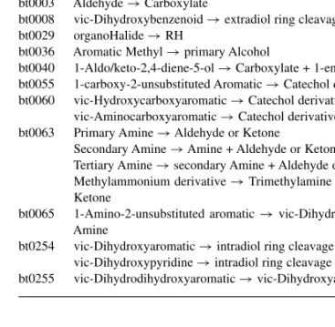
Table 1. List of the 13 transformation rules in the subset used for prediction Rule Description
bt0001 Primary Alcohol→ Aldehyde bt0002 Secondary Alcohol→ Ketone Secondary Alcohol→ Ester bt0003 Aldehyde→ Carboxylate
bt0008 vic-Dihydroxybenzenoid→ extradiol ring cleavage bt0029 organoHalide→ RH
bt0036 Aromatic Methyl→ primary Alcohol
bt0040 1-Aldo/keto-2,4-diene-5-ol→ Carboxylate + 1-ene-4-one bt0055 1-carboxy-2-unsubstituted Aromatic→ Catechol derivative bt0060 vic-Hydroxycarboxyaromatic→ Catechol derivative
vic-Aminocarboxyaromatic→ Catechol derivative bt0063 Primary Amine→ Aldehyde or Ketone
Secondary Amine→ Amine + Aldehyde or Ketone Tertiary Amine→ secondary Amine + Aldehyde or Ketone Methylammonium derivative→ Trimethylamine + Aldehyde or Ketone
bt0065 1-Amino-2-unsubstituted aromatic→ vic-Dihydroxyaromatic + Amine
bt0254 vic-Dihydroxyaromatic→ intradiol ring cleavage vic-Dihydroxypyridine→ intradiol ring cleavage bt0255 vic-Dihydrodihydroxyaromatic→ vic-Dihydroxyaromatic
the ratio of positive examples, all structures are predicted as positive, i.e. they are predicted to trigger this transformation rule correctly.
For the computation of frequently occurring molecular fragments, we applied the FreeTreeMiner system (Rückert and Kramer, 2004), as it builds on a computer chemistry library to handle structures and substructures conveniently.
4 PERFORMANCE MEASURES
Clearly, we are facing a fundamental trade-off also found in many other applications of machine learning and classification: if the
rules are too general, we will not miss many positive examples, but we might also include too many false positives. Vice versa, if the rules are too specific, we probably have few false positives, but we will potentially miss too many positives. It is convenient to think of this trade-off in terms of recall (sensitivity) and precision (selectivity). If the overall system predicts an observed product for a given substrate, we can count this as a true positive. If the system predicts a product that is not observed, we have a false positive. If a product is missing for a substrate, we have a false negative.2
The number of true positives is denoted by TP, the number of false positives by FP and the number of false negatives by FN. Then the standard definitions of recall (sensitivity) and precision (selectivity) can be applied:
R=Sensitivity = TP
TP+FN
P=Selectivity = TP
TP+FP
The overall number of products predicted by the system critically
depends on the cut-off parameterθ. To evaluate the performance
of the system, this parameter does not need to be fixed in advance. Instead, the parameter can be varied over the whole range from 0 to 1, and the resulting values for R and P can be plotted in two dimensions: recall is plotted on the x-axis and precision on the y-axis. Recall–precision plots offer an easy and intuitive visualization of the trade-offs involved in choosing a certain value ofθ. Also the results of approaches without cut-off parameters (e.g. relative reasoning as discussed above) appear as single data points in recall–precision space.
Recall–precision analysis can be performed on the system level as well as on the level of individual rules. In principle, one could set the threshold individually for each rule, but this would introduce a large number of parameters. For simplicity, we chose to visualize the system’s performance below by applying the same threshold for all rules. Also, as individual classifier schemes should be sensitive and adaptive to different class distributions, one parameter for all should work reasonably well in the first approximation.
In addition to recall–precision analysis, we measure the area under the receiver operating characteristic (ROC) curve, which indicates the capability of a classifier to rank the examples correctly (Cortes and Mohri, 2004).
5 EXPERIMENTAL RESULTS
In the following, we present the experimental results obtained with our approach. After introducing various learning schemes and settings, we present the results on the xenobiotics test set and, more importantly, our main results from a leave-one-out cross-validation over the UM-BBD structures.
For the 13 transformation rules in the subset, we applied the Random Forest algorithm (Breiman, 2001) in the implementation
2We count the false negatives in a slightly different way than in a previous
paper (Fenner et al., 2008), as we only consider products that are suggested by any of the biotransformation rules. In other words, we do not take into account products of reactions that are not subsumed by any of the rules. This is done because only for the products suggested by the UM-PPS, the method proposed here becomes effective—the classifiers can only restrict the rules, not extend them.
of the Weka workbench (Witten and Frank, 1999), because it gave good probability estimates in preliminary experiments. As a second classifier, we used Support Vector Machines (SVMs) trained using sequential minimal optimization (Platt, 1999a) in the implementation of the Weka workbench. We automatically adjusted the complexity constant of the support vector machine for each transformation rule separately. We used a 10-fold cross-validation to generate the data for the logistic models (Platt, 1999b) to obtain well-calibrated class probability estimates.3For the DC on the remaining
118 transformation rules, we used the ZeroR algorithm of the Weka workbench.
In total, we evaluated three variants:
(a) 13 learned classifiers (LC) (i.e. Random Forests or SVMs) only,
(b) 13 LCs and 118 DC and (c) 131 LCs (without DCs).
The idea of (a) is to evaluate the performance of the machine learning component of the system only. In (b), the overall performance of the system is evaluated, where 13 classifiers are complemented by 118 DCs. The purpose of (c) is to show whether the DCs are really sufficient, or whether LCs should be used even when samples are very small and classes are unequally distributed. All the results are shown in terms of manually chosen points in recall–precision space (e.g. before inflection points) as well as the area under the ROC curve (AUC). The possibility to choose thresholds manually is one of the advantages of working in recall–precision and ROC space: instead of fixing the precise thresholds in advance, it is possible to inspect the behavior over a whole range of cost settings, and set the threshold accordingly. Finally, we compare the results to the performance of relative reasoning.4
For compatibility with a previous paper (Fenner et al., 2008), we start with the results of training on all UM-BBD compounds and testing on the set of 25 xenobiotics. The results are given in the upper part of Table 2. It should be noted that in this case the DCs were ‘trained’ on the class distributions of the UM-BBD training data, and subsequently applied to the external xenobiotics test set.
First, we observe that ROC scores are on a fairly good level. The results in recall–precision space indicate that variant (b) is as good
as variant (c). However, with an AUC of∼0.5, having 13 LCs only
[variant (a)], performs on the level of random guessing. An indepth comparison of the two sets of structures (UM-BBD and xenobiotics) shows that this can be attributed to (i) the low structural similarity between the two sets, and (ii) the fact that a very limited set of rules trigger at all for the xenobiotics [a consequence of (i)]. The average number of free tree substructures per compound is 48.76 in the xenobiotics dataset, whereas it is 65.24 in the UM-BBD dataset. Due to this structural dissimilarity, the transfer from one dataset to the other is a hard task. Therefore, we decided to perform a leave-one-out cross-validation over all UM-BBD compounds, where the
3It should be noted that any other machine learning algorithm for
classification and, similarly, any other method for the computation of substructural or other molecular descriptors could be applied to the problem.
4We cannot compare our results with those of CATABOL, because the system
is proprietary and cannot be trained to predict the probability of individual rules—the pathway structure has to be fixed for training (for details we refer to Section 6). This means that CATABOL addresses a different problem than the approach presented here.
Table 2. Recall and precision for one threshold (on the predicted probability of being in the positive class) of the machine learning approach and for relative reasoning
Method Variant LC DC θ Recall Precision AUC
Xeno- RF (a) 13 0 0.417 0.400 0.333 0.505 biotics RF (b) 13 118 0.296 0.525 0.447 0.676 RF (c) 131 0 0.35 0.475 0.404 0.664 SVM (a) 13 0 0.023 0.800 0.235 0.389 SVM (b) 13 118 0.296 0.475 0.463 0.674 SVM (c) 131 0 0.157 0.410 0.390 0.599 RR – – – – 0.950 0.242 – UM- RF (a) 13 0 0.600 0.777 0.788 0.902 BBD RF (b) 13 118 0.308 0.595 0.594 0.842 RF (c) 131 0 0.485 0.653 0.632 0.857 SVM (a) 13 0 0.329 0.813 0.771 0.903 SVM (b) 13 118 0.294 0.582 0.588 0.841 SVM (c) 131 0 0.250 0.632 0.623 0.833 RR – – – – 0.942 0.267 –
The columns LC and DC indicate the number of transformation rules used for the LC, SVMs or Random Forests, and the DC, ZeroR. The value ofθ is determined manually considering the trade-off between recall and precision. We chose the threshold manually at an approximate optimum for recall and precision to provide a comparison to previous work (Fenner et al., 2008). AUC is threshold independent and only given for the new approach. The column with the variant refers to the assignment of rules to the different classifiers and is explained in the text.
structural similarity between test and training structures is higher than in the validation with the 25 xenobiotics as test structures.
Our main results from leave-one-out over the UM-BBD compounds are visualized in the recall–precision plots of Figure 3 and shown quantitatively in Table 2. Figure 3a and b shows the plots of the Random Forest classifiers and Figure 3c and d displays the results of the SVMs. Figure 3a and c shows the results of the classifiers on the 13 transformation rules in the subset and Figure 3b and d uses the DC for the remaining rules. The plots tend to flatten while including predictions of the DC. The overall performance does not differ too much between Random Forest and SVMs. Using both classification methods, we can achieve recall and precision of slightly less than 0.8 (see Fig. 3a and c and also the values for 13+0 in the lower part of Table 2) for the LC only in a leave-one-out cross-validation. The quantitative results in Table 2 also show that the performance of Random Forests and SVMs are on a similar level. Also in this case, the performance of LCs complemented by DCs is nearly as good as the performance of the LCs for all rules, supporting the idea of having such a mixed (LC and DC) approach.5However, in this case, the machine learning component
consisting of 13 LCs only, as expected, performs better on average than the overall system with 118 DCs added. In summary, the AUC scores are satisfactory, and the recall–precision scores of∼0.8 of the machine learning component show that improvements in precision are possible without compromising recall too much. Therefore, the machine learning approach provides some added value compared with the relative reasoning approach developed previously (Fenner
et al., 2008).
5In other words, it shows that informed classifiers do not pay off for the rest
of the rules. 0 0.2 0.4 0.6 0.8 1 0 0.2 0.4 0.6 0.8 1 Precision Recall 0.0 0.1 0.2 0.3 0.4 0.5 0.6 0.7 0.8 0.9 1.0 (a)
Random Forest, no default classifier 0 0.2 0.4 0.6 0.8 1 0 0.2 0.4 0.6 0.8 1 Precision Recall 0.0 0.1 0.2 0.3 0.4 0.5 0.6 0.7 0.8 0.9 1.0 (b)
Random Forest, default classifier
0 0.2 0.4 0.6 0.8 1 0 0.2 0.4 0.6 0.8 1 Precision Recall 0.0 0.1 0.2 0.3 0.4 0.5 0.6 0.7 0.8 0.9 1.0 (c) SVM, no default classifier 0 0.2 0.4 0.6 0.8 1 0 0.2 0.4 0.6 0.8 1 Precision Recall 0.0 0.1 0.2 0.3 0.4 0.5 0.6 0.7 0.8 0.9 1.0 (d) SVM, default classifier
Fig. 3. Recall–precision plots from a leave-one-out cross-validation using the Random Forest classifier (a and b) and SVMs (c and d). On the left-hand side (a and c), only the results of classifiers on a subset of the rules is shown. On the right-hand side (b and d), classifiers were generated for the same subset and a DC is used for the remaining rules. The subset was chosen by using transformation rules with at least 35 triggered examples and a minimum ratio of known products of 0.15. Using these parameters, 13 transformation rules were selected. The thresholdθ is given in 10 steps per plot. Note that the points in recall–precision space are connected by lines just to highlight their position: in contrast to ROC space, it is not possible to interpolate linearly.
To evaluate the enhancement of using both the structural information and the expert knowledge in the transformation rules, we applied the new method individually to the dataset leaving out the structure and, in a second run, the transformation rules. As it tends to give smoother probability estimates, we focus on Random Forest classifiers here and in the remainder of the section. Using only the structural information gives an AUC of 0.895, whereas the transformation rules only give an AUC of 0.885. Taken together, we can observe an AUC of 0.902, which, despite the apparent redundancy for the given dataset, marks an improvement over the results of the individual feature sets.
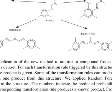
An example prediction of the biotransformation of a structure is given in Figure 4. We applied our approach to amitraz, a pesticide from the xenobiotics dataset. The incorrectly triggered transformation rules all get a rather low probability, while bt0063, a correctly triggered rule, is the only transformation rule being predicted with a probability higher than 0.53. As the xenobiotics dataset is very small, we generated Random Forest classifiers for every transformation rule triggered by this structure for the purpose of the example.
6 DISCUSSION AND CONCLUSION
We presented a combined knowledge- and machine learning-based approach to the prediction of biodegradation products and pathways. The proposed solution performs relative reasoning in a machine learning framework. One of the advantages of the approach is that probability estimates are obtained for each biotransformation rule.
N N N Amitraz N N N HO OH bt0005: 0.0 N N N HO bt0011: 0.16 N N N OH bt0012: 0.0 N N N OH bt0013: 0.033 N N N HO bt0036:0.2 N HN N bt0063: 0.6
Fig. 4. Application of the new method to amitraz, a compound from the xenobiotics dataset. For each transformation rule triggered by this structure, an example product is given. Some of the transformation rules can produce more than one product from this structure. We applied Random Forest classifiers to the structure. The numbers indicate the predicted probability that the corresponding transformation rule produces a known product. From the transformations predicted by the UM-PPS, only bt0063 produces a known product. As shown in the figure, this is the only transformation rule with a relatively high predicted probability.
Thus, the results are tunable and can be analyzed in recall– precision space. Making the trade-off between recall (sensitivity) and precision (selectivity) explicit, one can choose whether one or the other is more important.
In contrast to CATABOL, the approach works on the level of rules and not on the level of pathways. In CATABOL, the structure of pathways has to be laid out in advance in order to solve the equations based on the training data. To make the computations more stable, reactions have to be grouped using expert knowledge. In contrast, we apply the rules to the training structures to extract a matrix, which is the basis for the creation of the training sets for each rule. CATABOL learns parameters for a fixed pathway structure, whereas the approach proposed here learns classifiers for (individual) transformation rules. During testing, only the pathways laid out for training can be used for making predictions in CATABOL. In contrast, the approach presented here predicts one transformation after the other according to the rules’ applicability and priority determined by the classifiers. Overall, the training of CATABOL requires more human intervention than our approach, e.g. for grouping and defining hierarchies of rules (Dimitrov et al., 2004).
One might speculate (i) which other methods could be used to address this problem, and (ii) where the proposed solution could be applied elsewhere. Regarding (i), it appears unlikely that human domain experts would be able and willing to write complex relative reasoning rules as the ones derived in this work. Alternatively, other machine learning schemes could be used to solve the problem, for instance, methods for the prediction of structured output (Joachims
et al., 2009) or multi-label classification (Tsoumakas et al., 2009).
Methods for the prediction of structured output should be expected
to require a large number of observations to make meaningful predictions. Also, with the availability of transformation rules, the output space is already structured and apparently much easier to handle than the typically much less-constrained problem of structured output. Since multi-label classification seems particularly promising to address the problem described here, we are planning to investigate its use in future work. Regarding (ii), the approach could be used wherever expert-provided over-general transformation rules need to be restricted and knowledge about transformation products is available. It would be tempting to use the same kind of approach for other pathway databases like KEGG, if they were extended toward pathway prediction systems such as the UM-BBD. Our extended pathway prediction system could also be used as a tool in combination with toxicity prediction, as the toxicity of transformation products often exceeds the toxicity of their parent compounds (Sinclair and Boxall, 2003). The procedure would be first to predict the degradation products and then use some (Q)SAR model to predict their toxicity.
Currently, we are integrating the resulting approach into an experimental version of the UM-PPS server. In the future, it may become necessary to adapt the method to more complex rule sets, e.g. (super-)rules composed of other (sub-)rules. Such complex rule sets should be useful for the representation of cascades of reactions.
Funding: Fellowship for advanced researchers from the Swiss
National Science Foundation (PA002-113140 to K.F.), Lhasa Limited, the US National Science Foundation (NSF0543416); the University of Minnesota Supercomputing Institute. EU FP7 project OpenTox Health-F5-2008-200787.
Conflict of Interest: none declared.
REFERENCES
Breiman,L. (2001). Random forests. Mach. Learn., 45, 5–32.
Button,W.G. et al. (2003) Using absolute and relative reasoning in the prediction of the potential metabolism of xenobiotics. J. Chem. Inf. Comput. Sci., 43, 1371–1377.
Cortes,C. and Mohri,M. (2004) AUC optimization vs. error rate minimization. In Advances in Neural Information Processing Systems 16. MIT Press, Vancouver, Canada.
Dimitrov,S. et al. (2004) Predicting the biodegradation products of perfluorinated chemicals using catabol. SAR QSAR Environ. Res., 1, 69–82.
Dimitrov,S. et al. (2007) A kinetic model for predicting biodegradation. SAR QSAR Environ. Res., 18, 443–457.
Ellis,L.B. et al. (2006) The university of minnesota biocatalysis/biodegradation database: the first decade. Nucleic Acids Res., 34, D517–D521.
Fenner,K. et al. (2008) Data-driven extraction of relative reasoning rules to limit combinatorial explosion in biodegradation pathway prediction. Bioinformatics, 24, 2079–2085.
Gomez,M.J. et al. (2007) The environmental fate of organic pollutants through the global microbial metabolism. Mol. Syst. Biol., 3, Article number 114.
Greene,N. et al. (1999) Knowledge-based expert systems for toxicity and metabolism prediction: DEREK, StAR and METEOR. SAR QSAR Environ. Res., 10, 299–314.
Hou,B.K. et al. (2004) Encoding microbial metabolic logic: predicting biodegradation. J. Ind. Microbiol. Biotechnol., 31, 261–272.
Joachims,T. et al. (2009) Predicting structured objects with support vector machines. Commun. ACM, 52, 97–104.
Klopman,G. et al. (1997) Meta 3 a genetic algorithm for metabolic transform priorities optimization. J. Chem. Inf. Comput. Sci., 37, 329–334.
Mu,F. et al. (2006) Prediction of oxidoreductase-catalyzed reactions based on atomic properties of metabolites. Bioinformatics, 22, 3082–3088.
Platt,J.C. (1999a) Fast training of support vector machines using sequential minimal optimization. In Advances in Kernel Methods: Support Vector Learning. MIT Press, Cambridge, MA, pp. 185–208.
Platt,J.C. (1999b) Probabilistic outputs for support vector machines and comparisons to regularized likelihood methods. In Advances in Large Margin Classifiers. MIT Press, Cambridge, MA.
Rückert,U. and Kramer,S. (2004) Frequent free tree discovery in graph data. In SAC’04: Proceedings of the 2004 ACM symposium on applied computing. ACM Press, New York, NY, pp. 564–570.
Sinclair,C. and Boxall,A. (2003) Assessing the ecotoxicity of pesticide transformation products. Environ. Sci. Technol., 37, 4617–4625.
Tsoumakas,G. et al. (2009) Mining multi-label data. In Data Mining and Knowledge Discovery Handbook, 2nd edn. Springer.
Witten,I.H. and Frank,E. (1999) Data Mining: Practical Machine Learning Tools and Techniques with Java Implementations. Morgan Kaufmann, San Francisco, CA.