The Representation of the Visual Field in Three Extrastriate Areas of the Ferret (Mustela putorius) and the Relationship of Retinotopy and Field Boundaries to Callosal Connectivity

Texte intégral

(1)The Representation of the Visual Field in Three Extrastriate Areas of the Ferret (Mustela putorius) and the Relationship of Retinotopy and Field Boundaries to Callosal Connectivity. We describe representations of the visual field in areas 18, 19 and 21 of the ferret using standard microelectrode mapping techniques. In all areas the azimuths are represented as islands of peripheral visual field surrounded by central visual field representation. The zero meridian was found at the 17/18 and 19/21 borders; at the 18/19 and anterior border of 21 the relative periphery of the visual field was found. In areas 18 and 19, elevations are represented in a smooth medio-lateral progression from lower to upper visual field. In several cases the elevations in area 21 evidenced a similar medio-lateral progression; however, in others the elevations exhibited a split representation of the horizontal meridian. Anatomically determined callosal connections coincided with the representation of azimuths near the zero meridian. Medio-lateral bands of callosal connectivity that straddle the 17/18 and 19/21 borders are connected by bridges of callosally projecting cells. Acallosal cortical islands corresponded to the peripheral visual field and were found straddling the 18/19 border and the anterior border of area 21. The results are discussed in relation to callosal connectivity and retinotopy in extrastriate visual cortex and to proposed homologies of carnivore and primate visual cortex.. Introduction Despite being comprised of 271 extant species with complex brain structure (Radinsky, 1969; Wozencraft, 1993), the only carnivore species in which the extrastriate cortex has been thoroughly studied is the domestic cat (Payne, 1993; Pigarev and Rodionova, 1998). The ferret is a member of the canid lineage, whereas the cat is a member of the felid lineage and thus diverged ∼55 million years ago (Bininda-Emonds et al., 1999). One might expect differences between these species; however, the similarities may ref lect general principles of organization of the carnivore visual system. A better understanding of carnivore visual cortex is important for understanding the evolution of the primate visual system (Payne, 1993; Pigarev and Rodionova, 1998). Some aspects of the organization of the visual areas are revealed by the distribution of callosal connections. Callosal connections have been shown to correlate with the representation of the vertical meridian at the striate–peristriate border of several species (Montero et al., 1973; van Essen and Zeki, 1978; Jen et al., 1984) [reviewed in (Innocenti, 1986; Olavarria and Montero, 1989)]. From this observation, it was predicted that the callosal connections should indicate regions of vertical meridian representation in extrastriate visual areas and therefore their borders (van Essen and Zeki, 1978; Olavarria and Montero, 1984; Thomas and Espinoza, 1987; Martinich et al., 2000). However, the distribution of callosal connections in extrastriate areas, including the ferret (Innocenti et al., 2002), exhibit a complicated pattern and so it seems unlikely that they relate to areal borders in any simple way. In the previous paper (Innocenti et al., 2002), we proposed that callosal connectivity would correlate to both areal borders and anisotropies in the repre© Oxford University Press 2002. All rights reserved.. Paul R. Manger1, Daniel Kiper2,3, Italo Masiello1, Luis Murillo2, Laurent Tettoni2, Zsolt Hunyadi1 and Giorgio M. Innocenti1,2 1 Department of Neuroscience, Division of Neuroanatomy and Brain Development, Karolinska Institutet, Retzius väg 8, S-171 77 Stockholm, Sweden and 2Institute of Cell Biology and Morphology, University of Lausanne, CH-1005, Switzerland 3 Current address: Institute of Neuroinformatics, University/ETH Zurich, 8057 Zurich, Switzerland. sentation of the visual field within cortical areas. If this were so, it may lead to the reinterpretation of the relationship of callosal connections to area borders in other species, for example in rodents, for which the identification of cortical areas based on the combination of mapping and callosal connectivity has lead to controversial interpretations (Olavarria and Montero, 1984; Rosa and Krubitzer, 1999). Using standard microelectrode mapping procedures to determine cortical boundaries, combined with anatomical tracing from the contralateral hemisphere to indicate callosal connections, we examined three questions of interest. First, we compare the organization of extrastriate cortex with that of the domestic cat and other species. Second, the predictive value of callosal connectivity in regards to extrastriate cortical field boundaries is tested. Finally, we examine the relationship between callosal connectivity and retinotopy within extrastriate visual areas.. Materials and Methods Twenty adult female ferrets (Mustela putorius, 600–1000 g) were used. A ll experiments were performed according to Swedish, Swiss and European Community guidelines for the care and use of animals in scientific experiments. Two series of experiments were undertaken: plain electrophysiological mapping (15 cases) and mapping combined with tracing of callosal connections (five cases). Anatomical methods are described in the companion paper (Innocenti et al., 2002). Electrophysiological Recordings For the electrophysiological experiments, the animals were initially anesthetized with ketamine hydrochloride (Ketalar, 10 mg/kg, i.m.), medetomidin hydrochloride (Domitor, 0.08 mg/kg, i.m.), supplemented with atropine sulphate (0.15 mg/kg, i.m.). After inserting a cannula into the femoral vein and a tracheal tube (5 mm diameter), the animal was placed in a stereotaxic frame. The animal was artificially ventilated and anesthetized with 1% isof lurane in 1:1 nitrous oxide and oxygen. The expired CO2 was maintained between 3.5 and 4.0%, body temperature between 37 and 38°C, and the heart rate noted periodically to ensure stability of the animal. The visual cortex was exposed and protected with viscous mineral oil or with a layer of 3% agar. When the hemispheric screen was used, two orthopedic screws were inserted into the cranial vault and attached to the end of a stainless steel rod mounted to the stereotaxic frame, allowing removal of the stereotaxic frame. In cases when a tangent screen was used, the animal was left in the stereotaxic frame. The animal was paralysed with an initial intravenous bolus of pancuronium bromide (0.15 mg/kg), supplemented with a continuous infusion of pancuronium bromide (6 µg/kg/h, 1.5 mg in 25 ml normal saline). The pupil was dilated (1% atropine) and a contact lens was placed over the eye. Using a reversible ophthalmoscope, the position of the optic disk (contralateral to the exposed hemisphere) was marked onto a translucent tangent screen (57 cm from the eye), or hemispheric screen (45 cm radius) positioned to cover the entire visual field. The optic disk was found 15° above the horizontal meridian as seen previously (Law et al., 1988) and, on average, Cerebral Cortex Apr 2002;12:423–437; 1047–3211/02/$4.00.

(2) 35° from the zero meridian. Repeated recordings at a single location in most experiments ensured that eye position drift was minimal (<2°). Varnish-insulated tungsten microelectrodes (0.95–1.3 MΩ, exposed tip of ∼15 µm), were inserted orthogonal to the pial surface to depths between 500 and 1000 µm. Individual penetrations were separated by 250–500 µm anteroposteriorly and 700–1400 µm medio-laterally (depending on vasculature). Their position was marked on a photograph of the cortical surface. The electrophysiological signal was amplified and filtered, visualized on an oscilloscope and played through a loudspeaker. Minimal receptive fields (RFs) were defined by moving or f lashing luminous white circles (1° and 20° diameter) across the surface of the screen. Since clusters of neurons, not single units, were recorded, a systematic study of orientation and direction bias was not undertaken. Recording sites, the majority of which were visible in the processed tissue (Fig. 1), were aligned with architectural features, labeled cells and axons. Histology At the conclusion of the recording session, the animals were killed, fixed and the cerebral cortices processed as described in the companion paper (Innocenti et al., 2002). In purely electrophysiological mapping experiments, sections of the cerebral cortex were stained for cytochrome oxidase (CO) and for combined tracing/mapping experiments, alternate sections were stained for CO, or reacted to visualize biotinylated dextran. Reconstruction of Connections and Maps For each tracing/mapping case a complete map of the callosal connections was generated (Innocenti et al., 2002). To identify recording sites, the CO stained sections were examined with a stereoscope and the recording sites (Fig. 1) and architectonic boundaries marked on a camera lucida drawing. In the tracing/mapping cases, the electrode tracks were used to align labelled cells and recordings. Areal physiological borders were determined by reversals in RF progressions, RF size changes and changes in the neuronal response properties (Fig. 2). To generate physiological maps we used two techniques. The first was manual reconstruction as is standard in studies of this kind and the second was computer-aided (Fig. 2). Information from each recording site was entered into Excel (Microsoft) and processed in Matlab V5 (MathWorks Inc.) as: azimuth (degrees from zero meridian), elevation (degrees above/below horizontal meridian) and RF sizes (horizontal and vertical diameters in degrees). In this study we used the zero meridian, defined as the most rostral azimuth of the leading edge of the combined RFs, in place of the vertical meridian. For azimuth and elevation, scaled circles were overlaid on the position of the recording site (using Image Mapper, written by Laurent Tettoni). For RF size, lines representing the width and height of the RF were overlaid onto the recording sites. This allowed immediate visualization of all parameters and their easy comparison with architectonic borders (e.g. Figs 2, 5 and 6).. Results We found three representations of the contralateral visual hemifield rostral to area 17, or V1 (Law et al., 1988); see Figure 3. These fields lie within the architectonically defined regions 18, 19 and 21 (Innocenti et al., 2002). The anterior border of area 18 is particularly clear in the semi-f lattened CO sections (Fig. 1). Isoelevation lines run antero-posteriorly in all three areas, with the lower visual field represented medially and the upper visual field laterally; however, in area 21 a more complex representation of elevations was often observed (see below). Representation of azimuths formed a complex island-and-bridge pattern, which we found was related to callosal connectivity. The zero meridian was located at the 17/18 and 19/21 borders, the relative periphery (see below) at the 18/19 border and the anterior border of area 21. Visuotopic Representation in area 18 The representation of the visual field within area 18 was determined in nine experiments. Elevations exhibit a smooth change as recordings sites move from medial (lower visual field). 424 Extrastriate Visual Areas of the Ferret • Manger et al.. Figure 1. Semi-flattened section of ferret occipital lobe reacted for cytochrome oxidase (CO). Areas 17 and 18 are the dense regions of CO reactivity (arrows mark the architectonic borders). This photograph demonstrates the tissue artefacts left by the recording electrode (arrowheads). The electrode tracks can be readily matched to cortical architecture in these preparations. This section is within 200 µm of the pial surface. Scale bar = 1 mm.. in area 18 to lateral (upper visual field); see Figures 4 and 9. Isoelevation lines run antero-posteriorly and are continuous with those found in area 17 (Law et al., 1988). Elevations 10° above and below the horizontal meridian have a greatly expanded representation and occupy a little more than one-third of this area. The representation of azimuths was far more complicated than that of the elevations. The zero meridian was located at the posterior border of area 18 (Figs 4 and 9). As recording sites progressed rostrally in area 18, RFs were located progressively toward the periphery, to an extent that varied with medio-lateral position in area 18. In some recording rows, RF centers were found as far peripheral as 120° (e.g. Fig. 4, rfs 8, 9), whereas in others they remained within 25° of the zero meridian (e.g. Fig. 4, rfs 19–22). These rows with small peripheral movements of the RFs were often adjacent to each other, forming bridges that stretched across area 18. The rows in which large azimuths were found delineated islands (Fig. 9). Despite some recordings rows showing limited azimuthal progression, the RFs recorded at the anterior border of area 18 were always more peripheral than those recorded more posteriorly. Thus, we can say that the anterior border of area 18 corresponds to a representation of the relative peripher y of the visual field. The representation of azimuths reversed around the anterior border of area 18 as recordings moved into areas 7 medially, 19 and temporal cortex laterally. A band of ipsilateral eye dominance (antero-posterior.

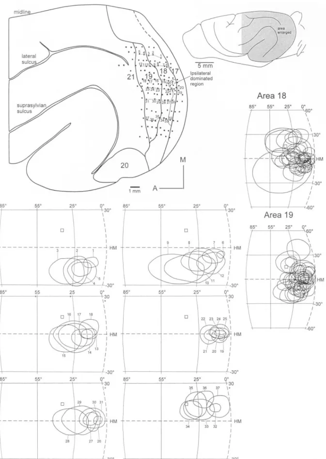
(3) Figure 2. Computer-based map reconstructions of the data from a single case. In the upper two diagrams elevations and azimuths are depicted. The diameters of the circles represent the degrees (see scale) in elevation (above/below the horizontal meridian) or azimuth (from the zero meridian). For elevations, the circles with thicker lines are above the horizontal meridian and those with thinner lines below. In the third diagram (lower left) RF sizes are shown. Vertical bars represent the RF size in elevation and horizontal bars represent the RF size in azimuth. The scale to the right shows the relative size of the bars in degrees. Area borders (thin lines) are congruent with several changes, including reversals in the progressions of azimuths and changes in RF size.. Cerebral Cortex Apr 2002, V 12 N 4 425.

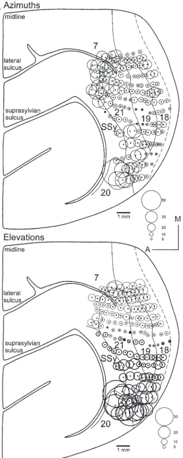
(4) Figure 3. Dorsolateral photograph of ferret brain with cortical field boundaries superimposed. Area 18 forms a thin band along the entire anterior border of area 17. Areas 19 and 21 are between area 18 and the suprasylvian sulcus. Other areal boundaries are based on exploratory recordings (dashed lines). Areas 3b and AI were identified on the basis of dense CO reactivity.. dimension of ∼500 µm, medio-lateral dimension of ∼5 mm), was found at the posterior border of area 18 (Fig. 4); see also Figure 4 in the companion paper (Innocenti et al., 2002), and White et al. (White et al., 1999). Within this band, neural responses could be driven by stimulation of both eyes; however, the responses evoked by stimulation of the ipsilateral eye were significantly stronger. In this region RFs were found with elevations 10° above and below the horizontal meridian and with maximal azimuths of 15° (Fig. 10). The extent of the visual field represented in area 18 covers elevations from 60° above to 50° below the horizontal meridian, with azimuths as peripheral as 120° from the zero meridian (Figs 4 and 7). The size of the RFs increased with eccentricity in the visual field (Fig. 8), but averaged ∼20° in azimuth and 10° in elevation. Visuotopic Representation in Area 19 The representation of the visual field within area 19 was determined in 12 experiments. As in area 18, the lower half of the visual field was found medially and the upper visual field laterally (Figs 4, 5 and 9). Elevations progressed smoothly in the medio-lateral direction. The isoelevation lines coursed antero-posteriorly and were continuous with those of area 18. Elevations 10° above and below the horizontal meridian occupied half of the representation. The zero meridian was found at the anterior border of area 19 (Figs 4, 5 and 9). As recording sites progressed caudally, RFs moved gradually into the periphery. In some recording rows, the RF centers did not move beyond 25° azimuth (e.g. Fig. 4, rfs 23–25; Fig. 5, rfs 7–9, 14–16), whereas in others they approached 70° (e.g. Fig. 4, rfs 10–12). The representation of azimuths formed an island-and-bridge pattern as seen in area 18. These islands and bridges were continuous with those found in area 18, thus the representation of azimuth in area 19 forms an approximate mirror image of area 18 (Fig. 9). The highest azimuths were invariably found along the posterior border of. 426 Extrastriate Visual Areas of the Ferret • Manger et al.. area 19. Thus, the 18/19 border represents the relative periphery of the visual field. The extent of visual field represented in area 19 covered elevations from 60° above to 50° below the horizontal meridian, with azimuths as peripheral as 70° (Figs 4, 5 and 7). The size of the RFs increased with eccentricity (Fig. 8), but averaged around 35° in azimuth and 20° in elevation. Visuotopic Representation in Area 21 Within area 21 of the ferret there were significant interindividual differences in the representation of the elevations; however, two clear patterns emerged. The first pattern, found in five cases, is that of a smooth progression of elevations from medial (lower visual field) to lateral (upper visual field) (Fig. 5). The representation of elevations within 10° above and below the horizontal meridian was expanded and occupied up to half of the area. In this first pattern, the isoelevation lines were continuous with those seen in area 19. The second pattern (seven cases) exhibited a split representation of the horizontal meridian (Fig. 6). Thus, as one moved from medial to lateral in area 21, RFs were initially recorded in the lower visual field and then progressed through the horizontal meridian, to ∼20° above it. At this point, the progression of elevations would reverse and the RFs moved closer to the horizontal meridian. Once the second representation of the horizontal meridian was reached, the progression would again reverse and RFs would be located at consistently higher elevations until the lateral edge of area 21 was reached. Despite these elevation reversals, there was only one representation of the visual field within area 21. This is due to the manner in which the azimuths are represented (see below). At the lateral border of area 21, elevations reversed around the upper limit of the visual field (Figs 5, 6 and 9). This reversal coincides with low myelin and CO staining and delineates the beginning of the temporal visual areas (Fig. 3). The retinotopy around the medial border of area 21 is complex due to its conf luence with areas 18.

(5) Figure 4. Reconstruction of the retinotopy within middle area 18 and all of area 19, with examples of RF progressions. Numbers at recording sites correspond to the illustrated RFs. Reversals in RF progressions correspond to area boundaries. In some rows, we see a substantial representation of the periphery; in others, the eccentricities of the RFs are quite small (contrast row labeled 1–5 with row labeled 6–12). A small band adjacent to the border with area 17 is dominated by ipsilateral eye input, but was weakly binocular. The figurines to the right show all the RFs recorded within areas 18 and 19 in the present case.. Cerebral Cortex Apr 2002, V 12 N 4 427.

(6) Figure 5(A). 428 Extrastriate Visual Areas of the Ferret • Manger et al..

(7) Figure 5. Reconstruction of the retinotopy within areas 19 and 21. Conventions as in Figures 2 and 4. (A) Area 21 represents more of the visual field than does area 19 (see figurines to the right). The internal topography of these areas can be visualized using both RF progressions (A) and circle diagrams (B). The circle diagram representing azimuths shows that the anterior border of area 21 represents the relative periphery, as does the posterior border of area 19. The peripheral representations fuse medially and laterally and continue along the anterior border of area 18. Elevations show a smooth medio-lateral progression of elevations in areas 18, 19 and 21. This is representative of a case of area 21 in which the representation of the horizontal meridian was not split.. Cerebral Cortex Apr 2002, V 12 N 4 429.

(8) Figure 6(A). 430 Extrastriate Visual Areas of the Ferret • Manger et al..

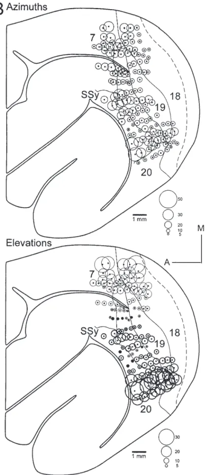
(9) Figure 6. Reconstruction of the retinotopy within area 21. Conventions as in Figures 2 and 4. In this case, a dual representation of the horizontal meridian is seen, both in the examples of RFs (A) and the circle diagrams (B). As recordings move medial to lateral in area 21, the elevations of the RFs begin in the lower visual field, pass through the horizontal meridian and progress to 20° above the horizontal meridian. At this point, RFs progress back to the horizontal meridian. Here again, retinotopy reverses and RFs are located progressively higher in the visual field until the lateral edge of area 21 is reached. Note that despite these reversals in elevation, a minimal portion of the visual field is re-represented due to the complicated azimuthal representation (see text).. Cerebral Cortex Apr 2002, V 12 N 4 431.

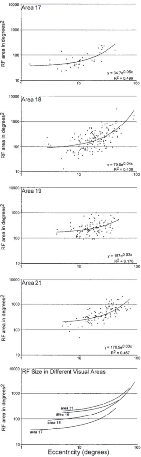
(10) Figure 7. Extent of visual field representation in each area compared to area 17 (Law et al., 1988). Area 18 has a slightly smaller representation of the visual field than area 17 (the surface delimited by the dashed line). Area 19 shows the most limited representation, with area 21 encompassing ∼20° more azimuth than area 19.. and 7; however, it became clear that the representations of the relative periphery of anterior 21 (see below), posterior 7 and that of the 18/19 border fused in this region. This is shown explicitly in Figures 5 and 6. The representation of azimuths is also complex in area 21. As with area 18 and 19, the representation of the zero meridian was consistent and was located at the posterior border of area 21 (Figs 5 and 6). As recording sites moved rostrally through area 21, RF centers shifted away from the zero meridian. In some recording rows, the RF centers approached 85° azimuth (e.g. Fig. 5, rfs 3–6, 31–34; Fig. 6, rfs 8–12, 19–22), while in others they did not exceed 30° (e.g. Fig. 5, rfs 25–28; Fig. 6, rfs 4–7, 13–15). Thus, a similar island-and-bridge pattern of azimuths, as seen in areas 18 and 19 was found, and the anterior border of area 21 coincides with a representation of the relative periphery. In cases with a simple representation of elevations, the azimuths exhibit a mirror reversal of that found in area 19 (Fig. 5). The anterior. 432 Extrastriate Visual Areas of the Ferret • Manger et al.. Figure 8. Plots of multiunit RF size (degrees2) against eccentricity. Eccentricity is given as the distance (in degrees) of the center of the RF from the intersection of the zero and horizontal meridians. The data were plotted in Excel and an equation describing the line of best fit and its correlation coefficient (R2) generated. In all areas, the size of the RF increased with eccentricity. The RF size within a cortical area increases from area 17, to 18, 19 and 21..

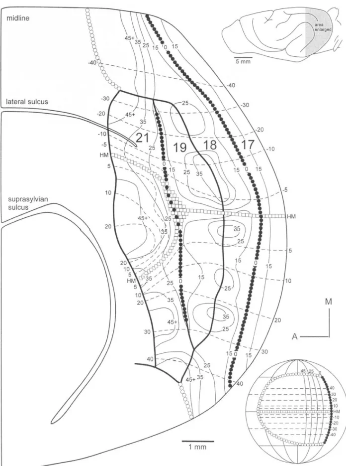
(11) Figure 9. Summary diagram of the retinotopy within the cortical areas investigated in the present study. Isoelevation lines progress smoothly in areas 17, 18 and 19. For this summary we chose to represent a case in which the horizontal meridian was duplicated in area 21 (see text). The representation of azimuth is complex in all three areas. Islands of peripheral representation straddle the 18/19 border and the anterior border of area 21. The zero meridian is consistently found at the 17/18 and 19/21 borders, but not at the medial and lateral edges of the 19/21 border. Numbers denote values of isoelevation (dashed lines) and isoazimuth (thin solid lines). Open squares represent the horizontal meridian (HM), filled circles the zero meridian (0) and open circles the periphery of the visual field (see globe figurine). This figure is an ‘average’ figure and is derived from several cases.. Cerebral Cortex Apr 2002, V 12 N 4 433.

(12) border of area 21 was adjacent to visually responsive regions in the posterior parietal cortex and the suprasylvian sulcus. Interestingly, in the cases with the split horizontal meridian representation, a small portion of the visual field seems to have a triple representation. In the case shown in Figure 6, this region was found between azimuths of 25° and 40°, and elevations of 0° and 20°. This was slightly variable between cases; however, the triple representation was restricted to a narrow portion of the visual field adjacent to, but above, the horizontal meridian (Fig. 9). Despite this region of triple representation, for the purposes of the present description we consider area 21 a single cortical area. In area 21, elevations from 60° above to 45° below the horizontal meridian were observed with representations of azimuth up to 85° (Figs 5, 6 and 7). There was a slight, but consistent, increase in the size of the RFs in area 21 as compared to area 19 (Fig. 8). As with the other cortical areas, the size of the RFs increased with eccentricity (Fig. 8), but on average a RF spanned 25–30° of azimuth and 30–35° of elevation. Thus, instead of being elongated along the horizontal, the RFs of neuronal clusters in area 21 often had axes of equal length, or the vertical axis was found to be slightly longer than the horizontal axis. Relationship of Callosal Connections to Retinotopy In five experiments, we combined the injections of tracer with recordings from the opposite hemisphere and related the pattern of labeling to the physiologically defined borders and area retinotopy. At the 17/18 border we consistently found that the callosally projecting neurons formed a band straddling the location of the zero meridian representation, by at least 0.5 mm on either side (Fig. 10). In mapping studies we found a second representation of the zero meridian at the 19/21 border (see above results). For the most part, the callosally projecting neurons formed a band straddling this border extending up to and >0.5 mm on either side (Fig. 10). In some cases the lateral and medial portions of the 19/21 border, at the conf luence of areas 18, 19 and 21, were not connected callosally. This correlates with our physiological finding that the peripheral representations fuse in these regions. Thus, while the callosal bands are a reliable indicator of the zero meridian representations, neither precisely corresponds to the areal borders. Callosal connections are uneven across ferret visual cortex (Innocenti et al., 2002). Acallosal islands were often found to straddle the 18/19 border (Fig. 10) as defined physiologically and anatomically (Innocenti et al., 2002). The mapping studies showed that within a cortical area, islands of peripheral representation alternated with bands of near zero meridian representation. We found that within the acallosal islands, the RF centers were located beyond 25° azimuth (Fig. 10). This is not a strict boundary and exceptional RF centers within the acallosal regions did have azimuths as small as 10° (Fig. 11). For the callosally connected regions, the majority of the RF centers were located between the zero meridian and 25° azimuth. However, RF centers located as far as 50° from the zero meridian were occasionally found, often in close proximity (<200 µm) to an acallosal region (Figs 10 and 11). The location of the leading edge of the RFs showed a similar result, with the majority of RFs located within a callosally connected region having a leading edge within 10° of the zero meridian and all within 20° of the zero meridian (Figs 10 and 11). The leading edge of RFs in acallosal regions were mostly found >10° from the zero meridian.. 434 Extrastriate Visual Areas of the Ferret • Manger et al.. Discussion The present study describes three representations of the visual field in the extrastriate visual cortex of the ferret. We term these areas 18, 19 and 21, rather than V2, V3 and V4, for three reasons. First, to conform to the standard nomenclature of extrastriate visual areas of the cat (Payne, 1993). Second, these representations correspond to the ferret architectonic regions 18, 19 and 21 (Innocenti et al., 2002). Third, the homologies of the areas between carnivore and primate species is still uncertain, thus we want to avoid inferring homology through terminology. To define the three areas, we used several criteria including: a single representation of the visual hemifield (both upper and lower quadrants); systematic reversals in the position of the RFs at borders of the areas; changes in RF size; and congruency of the retinal representation to architecture. We also found a relationship between the distribution of callosal connections, retinotopy and areal borders. Comparison to the Cat and other Species Law et al. described area 17 of the ferret (Law et al., 1988), which is virtually identical to that of the cat (Tusa et al., 1978) and very similar to other mammals (Rosa and Krubitzer, 1999). Rostral to area 17 we found a representation of the visual field in the architectonically defined area 18 (Innocenti et al., 2002). The retinotopy, topology, architecture and pattern of transneuronal labelling (Innocenti et al., 2002) all suggest that this area is homologous to cat area 18 (Donaldson and Whitteridge, 1977; Tusa et al., 1979; Albus and Beckmann, 1980; Berson and Graybiel, 1983). Moreover, it is likely to be homologous to V2 of other species (Rosa and Krubitzer, 1999). White et al. delineated a region of ferret area 18, adjacent to the 17/18 border, that is dominated by input from the ipsilateral eye (White et al., 1999). We have shown that this representation is a small band in the middle of area 18 at the 17/18 border (Fig. 4). This region is weakly binocular and not purely ipsilateral as previously described (White et al., 1999). The interpretation of White et al. may arise from the methodology, in that the use of optical imaging subtraction methods may have eliminated the weakly binocular character. The retinotopy, cortical location and architecture all suggest that ferret area 19 is homologous to cat area 19 (Heath and Jones, 1971; Donaldson and Whitteridge, 1977; Tusa et al., 1979; Albus and Beckman, 1980). Cat area 19 extends along the entire anterior border of area 18 (Albus and Beckmann, 1980). We find that both lateral and medial edges of area 19 of the ferret are foreshortened in comparison to that of the cat (Figs 3 and 9). This may represent a difference in the organization of the extrastriate cortex between the canids and the felids. Additionally, it appears that V3 (or carnivore area 19), forms part of the basic network of eutherian mammal visual cortex (Rosa, 1999), but see elsewhere (Kaas et al., 1972; Lyon et al., 1998). It should be noted here that the definition of V3 in primates is still a contentious issue, with several schema proposed (Gattass et al., 1988; Felleman and van Essen, 1991; Rosa and Tweedale, 2000). Of particular interest is the region described as areas 21a, 21b and 21c of the cat (Tusa and Palmer, 1980; Payne, 1993). Within architectonically defined area 21 of the ferret, in addition to the complex azimuthal representation, the retinotopy is often further complicated by a split in the representation of the horizontal meridian. In these cases it was difficult to define a single retinal representation within area 21 (Fig. 6), as a small portion of the visual field had a triple representation. This case of complex retinotopy in ferret area 21 appears very similar to that seen in cat areas 21a, 21b (Tusa and Palmer, 1980) and the.

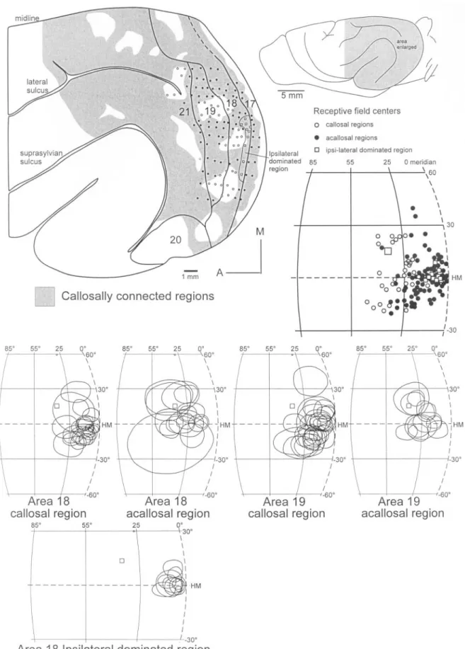
(13) Figure 10. Representation of the relationship between callosal connectivity and retinotopy. The regions containing labeled cells and axon terminals are shaded and show that callosal connections are uneven (Innocenti et al., 2002). Medio-lateral bands of connectivity straddle the 17/18 and the 19/21 borders. Within the acallosal regions, RFs are in the periphery of the visual field (i.e. azimuths >25°). In the figurine to the right, RF centers in the acallosal regions are shown as hollow circles, those in callosally connected regions as filled circles and those in the ipsilateral eye region of area 18 as hollow squares. The large hollow square shows the location of the optic disk. Note that RF centers in the callosally connected regions are located closer to the zero meridian. In the lower part of the figure, all RFs found in callosal and acallosal regions are shown. The leading edges of the RFs in the acallosal regions do not reach the zero meridian, unlike those in the callosal regions. Most conventions as in Figure 4.. Cerebral Cortex Apr 2002, V 12 N 4 435.

(14) ‘V4’ in primates (Gattass et al., 1988; Felleman and van Essen, 1991; Rosa and Tweedale, 2000). Payne has proposed that cat area 21 is homologous to V4 of the macaque monkey (Payne, 1993). The primate V4 exhibits a small amount of multiple representation (Gattass et al., 1988), similar to that of ferret and cat area 21 (Tusa and Palmer, 1980). However, a major problem for the proposal of Payne is that a V4 (or area 21) has not been reported for either the f lying fox (Rosa, 1999) or the tree shrew (Kaas et al., 1972; Lyon et al., 1998). As both are members of the archontans, which includes the primates, but specifically excludes the carnivores, an evolutionary quandary arises. We propose that V4 of primates and area 21 of carnivores each represent an independent evolution of a possibly analogous visual area. That V4 and area 21 have so many functional and connectional features in common (Payne, 1993) clearly indicates that they perform a substantially analogous function in the primate and carnivore visual systems.. Figure 11. Bar graphs showing the relationship of callosal connectivity with retinotopy. The RF centers in the callosally connected region fall mainly between 0 and 30° (upper graph). For the acallosal regions, the RF centers fall mainly above 20°. There is a significant region of overlap in the distribution of RF centers between 20 and 30° of azimuth. A similar situation is seen when the RF leading edge is graphed (lower graph). In callosally connected regions, the leading edges fall mostly between 0 and 5°; however, significant numbers are found up to 20°. The leading edges of RFs in the acallosal regions span the entire range of azimuths; however, most are found between 5 and 20°.. proposed 21c (Payne, 1993), with reversals around elevations within different parts of a single architectonic area. If we adopted a strict approach of separating cortical areas at all reversals in retinotopy, then in some cases we could propose three separate areas in ferret area 21. However, subdividing this region does not seem necessary. First, the region is architectonically homogeneous (Innocenti et al., 2002). Second, we would have to assume that cortical areas can have partial representations of the receptor surface. Third, in some cases there were no elevation reversals (Fig. 5), thus subdividing this region is not in agreement with all data. Fourth, in cases with elevation reversals, there was only a very limited amount of multiple representation due to the complicated layout of azimuth representation. Finally, as judged by multiunit recording, the region appears to be homogeneous in RF size and response properties. It has been proposed (Payne, 1993) that the areas described as 21a, 21b and Payne’s postulated 21c should be considered a single cortical area, cat area 21. Recent work (Pigarev and Rodionova, 1998) has provided evidence of a lower field representation in the postulated area 21c of Payne. Our results lead us to the conclusion that the ferret area 21 should be considered a single cortical area and support the proposal of Payne for the cat. Area 21 of the cat and ferret lies rostral to area 19 and caudal to the suprasylvian visual areas (possible analogues of the MT complex in primates). A similarly located area has been termed. 436 Extrastriate Visual Areas of the Ferret • Manger et al.. Cortical Area Borders, Retinotopy and Callosal Connectivity Particular portions of the visual field representations have been found at the borders of cortical areas. The most consistent finding across studies is the representation of the vertical, or zero, meridian at a particular edge of a cortical field. We found representations of the zero meridian at the 17/18 and 19/21 borders. We also found that medio-lateral bands of callosal connections, ∼1 mm wide, straddle these borders. These connections therefore do not give a precise location of the borders; however, they do validate the border location. The usefulness of callosal connectivity for defining areal borders is further limited by the complexity of the retinotopic representations, which is paralleled by the uneveness in callosal connectivity patterns. In particular, at the lateral and medial edges of the 19/21 border the retinotopy is complicated by the conf luence of cortical areas, 18, 19 and 21. At these locations we often found representations of the peripheral visual field, which coincided with a lack of callosal connections. Therefore, while callosal connections coincide with the middle portion of the 19/21 border, physiological mapping is needed to delineate this border, especially at its lateral and medial edges. A second complication in relating callosal connections to areal borders is that between the main bands of callosal connections at the 17/18 and 19/21 borders, callosally connected bridges alternate with acallosal islands. In the ferret these acallosal islands straddle cortical field boundaries, such as the 18/19 border and the anterior border of area 21. We now know, from combined anatomical and electrophysiological experiments, that the acallosal islands correspond to representations of the peripheral visual field. Within the callosally connected bridges a representation of the relative periphery was found. The notion of relative periphery is important in the interpretation of electrophysiological mapping results and their relation to callosal connections. While reversal in RF progression at borders of cortical fields is a general feature across mammals (Kaas, 1995), within the visual system, these reversals do not always correspond to the same degree of azimuth representation and were found to vary between 25° and 120° in the present study of the ferret. What are the possible reasons for the discontinuities in retinotopy and callosal connectivity we have reported here for the ferret? They might be the developmental consequence of mapping the visual field onto elongated cortical areas (Wolf et al., 1994). Models that imitate map formation in these areas bring about the island-and-bridge pattern we see from physio-.

(15) logical and anatomical experiments (Wolf et al., 1994). A lternatively, it has been proposed (Tusa and Palmer, 1980) that these transformations of the visual field are related to the advantage of shortening interconnections. Cortical areas which require a substantial amount of horizontal interaction benefit from shorter connections. It appears that constraints, both during development and for adult processing of visual information, are substantial factors that lead to the distorted represent of the visual field.. Notes The work reported in the present study was funded by grants to G.M.I. from the Swiss National Science Foundation (Grant PNR 38 No. 4038-043990), and the Swedish Medical Research Foundation (No. 12594). The authors wish to thank Ms Jenny Hedin for her consistent high-quality histological preparations used in the present study. Address correspondence to Giorgio Innocenti, Department of Neuroscience, Division of Neuroanatomy and Brain Development, Karolinska Institutet, Retzius väg 8, S-171 77 Stockholm, Sweden. Email: giorgio.innocenti@neuro.ki.se.. References Albus K, Beckmann R (1980) Second and third visual areas of the cat: interindividual variability in retinotopic arrangement and cortical location. J Physiol 299:247–276. Berson DM, Graybiel AM (1983) Organization of the striate-recipient zone of the cat’s lateralis posterior–pulvinar complex and its relations with the geniculostriate system. Neuroscience 9:337–372. Bininda-Emonds ORP, Gittleman JL, Purvis A (1999) Building large trees by combining phylogenetic information: a complete phylogeny of the extant Carnivora (Mammalia). Biol Rev 74:143–175. Donaldson IML, Whitteridge D (1977) The nature of the boundary between cortical visual areas II and III in the cat. Proc R Soc Lond B 199:445–462. Felleman DJ, Van Essen DC (1991) Distributed hierarchical processing in the primate cerebral cortex. Cereb Cortex 1:1–47. Gattass R, Sousa A PB, Gross CG (1988) Visuotopic organization and extent of V3 and V4 of the macaque. J Neurosci 8:1831–1845. Heath CJ, Jones EG (1971) The anatomical organization of the suprasylvian gyrus of the cat. Ergebn Anat EntwGesch 45:1–64. Innocenti GM (1986) General organization of the callosal connections in the cerebral cortex. In: Cerebral cortex (Jones EG, Peters A, eds), vol. 5, pp. 291–353. New York: Plenum Press. Innocenti GM, Manger PR, Masiello I, Colin I, Tettoni L (2002) Architecture and callosal connections of visual areas 17,18, 19 and 21 in the ferret (Mustela putorius). Cereb Cortex 12:411–422. Jen LS, So KF, Xiao YM, Diao YC, Wang YK, Pu ML (1984) Correlation between the visual callosal connections and the retinotopic organization in striate–peristriate border region in the hamster: an anatomical and physiological study. Neuroscience 13:1003–1010. Kaas JH (1995) The evolution of isocortex. Brain Behav Evol 46:187–196.. Kaas JH, Hall WC, Killackey H, Diamond IT (1972) Visual cortex of the tree shrew (Tupaia glis): architectonic subdivisions and representations of the visual field. Brain Res 42:491–496. Law MI, Zahs KR, Stryker MP (1988) Organization of the primary visual cortex (area 17) of the ferret. J Comp Neurol 278:157–180. Lyon DC, Jain N, Kaas JH (1998) Cortical connections of striate and extrastriate visual areas in tree shrews. J Comp Neurol 401:109–128. Martinich S, Pontes MN, Rocha-Miranda CE (2000) Patterns of corticocortical, corticotectal, and commissural connections in the opossum cortex. J Comp Neurol 416:224–244. Montero VM, Bravo H, Fernandez V (1973) Striate–peristriate corticocortical connections in the albino and gray rat. Brain Res 53:202–207. Olavarria J, Montero VM (1984) Relation of callosal and striate– extrastriate cortical connections in the rat: morphological definition of extrastriate visual areas. Exp Brain Res 54:240–252. Olavarria J, Montero VM (1989) Organization of visual cortex in the mouse revealed by correlating callosal and striate–extrastriate connections. Vis Neurosci 3:59–69. Payne BR (1993) Evidence for visual cortical area homologs in cat and macaque monkey. Cerebr Cortex 3:1–25. Pigarev IN, Rodionova EI (1998) Two visual areas located in the middle suprasylvian gyrus (cytoarchitectonic field 7) of the cat’s cortex. Neuroscience 85:717–732. Radinsky LB (1969) Outlines of canid and felid brain evolution. Ann NY Acad Sci 167:277–288. Rosa MGP (1999) Topographic organization of extrastriate areas in the f lying fox: implications for the evolution of mammalian visual cortex. J Comp Neurol 411:503–523. Rosa MGP, Krubitzer LA (1999) The evolution of visual cortex: where is V2? Trends Neurosci 22:242–248. Rosa MGP, Tweedale R (2000) Visual area in lateral and ventral extrastriate cortices of the marmoset monkey. J Comp Neurol 422: 621–651. Thomas HC, Espinoza SG (1987) Relationships between interhemispheric cortical connections and visual areas in hooded rats. Brain Res 417: 214–224. Tusa RJ, Palmer LA (1980) Retinotopic organization of areas 20 and 21 in the cat. J Comp Neurol 193:147–164. Tusa RJ, Palmer LA, Rosenquist AC (1978) The retinotopic organization of area 17 (striate cortex) in the cat. J Comp Neurol 177:107–128. Tusa RJ, Rosenquist AC, Palmer LA (1979) Retinotopic organization of areas 18 and 19 in the cat. J Comp Neurol 185:657–678. van Essen DC, Zeki SM (1978) The topographic organization of rhesus monkey prestriate cortex. J Physiol (Lond) 277:193–226. White LE, Bosking WH, Williams SM, Fitzpatrick D (1999) Maps of central visual space in ferret V1 and V2 lack matching inputs from the two eyes. J Neurosci 19:7089–7099. Wolf F, Bauer H-U, Geisel T (1994) Formation of field discontinuities and islands in visual cortical maps. Biol Cybern 70:525–531. Wozencraft WC (1993) Order Carnivora. In: Mammal species of the world: a taxonomic and geographic reference (Wilson DE, Reeder DA, eds), pp. 279–348. Washington, DC: Smithsonian Institution Press.. Cerebral Cortex Apr 2002, V 12 N 4 437.

(16)