Document Room, 20B-221
Besearch Laboratory of Electronlic Massachusetts Institute of echnology
MASSACHUSETTS INSTITUTE OF TECHNOLOGY RESEARCH LABORATORY OF ELECTRONICS
Technical Report No. 181
LOAA/
APPLICATION OF STATISTICAL METHODS TO COMMUNIC N PROBLEMS
Y. W. Lee
Abstract
The basic ideas and tools in the statistical theory of communication are discussed. The methods of the theory in the formulation of some important communication problems
are outlined. Some techniques which have been developed for application to practical
problems, and certain laboratory results in support of the theory are described. To
indicate the possibility of practical application, primarily with respect to improvement of signal-to-noise ratio, experimental results are presented.
September 1, 1950
5!X-F'-
C
The research reported in this document was made possible through support extended the Massachusetts Institute of Tech-nology, Research Laboratory of Electronics, jointly by the Army Signal Corps, the Navy Department (Office of Naval Research) and the Air Force (Air Materiel Command), under Signal Corps Contract No. W36-039-sc-32037, Project No. 102B; Department of the Army Project No. 3-99-10-022.
CONTENTS
Introduction 1
1. Time Functions in a Communication System 1
2. Generalized Harmonic Analysis 2
(a) Periodic Functions 2
(b) Aperiodic Functions 6
(c) Random Functions 7
(d) Summary 13
3. Measurement of Correlation Functions 15
4. Characterization of a Random Process 17
5. Separation of Periodic and Random Components 21
6. Filtering and Prediction 23
7. Use of Random Noise in System Characteristic Determination 25
APPLICATION OF STATISTICAL METHODS TO COMMUNICATION PROBLEMS Introduction
A significant advance in communication engineering in recent years is the development of a theory of communication in which the methods and techniques of the statistician have
augmented those of the communication engineer. The basis for the new development is
the concept that the flow of information, which is the primary concern of a communica-tion system, is a statistical phenomenon. In addicommunica-tion to providing effective and practical methods for the solution of a number of problems which have faced considerable difficulty under classical theory, statistical theory in the present state of development has already indicated the need and the method for recasting certain accepted theories. It has also indicated the possibility of new and effective systems of transmission, reception, and detection.
Among the many contributors in the new field of development is Norbert Wiener. His work on generalized harmonic analysis (ref. 1), his theory of statistical filtering and pre-diction (ref. 2), and his theory of cybernetics (ref. 3) have had a measure of influence in most of the recent work of other contributors.
In this paper the basic ideas and tools in the statistical theory are discussed. The methods of the theory in the formulation of some important communication problems are
outlined. Some techniques which have been developed for application to practical problems,
and certain laboratory results in support of the theory are described. To indicate the possibility of practical application, primarily with respect to improvement of signal-to-noise ratio, experimental results are presented.
1. Time Functions in a Communication System
In a communication system, varying quantities such as currents and voltages, dis-tributed in time, are processed during their passage through the system in a multitude of ways for the purpose of producing the desired results. Time functions also serve as processing agents within the system. These functions, which are usually continuous, may be classified as periodic, aperiodic, and random.
Among the great variety of functions which a periodic wave performs in a
communica-tion system, it carries informacommunica-tion, as it does for instance in a pulse-type radar set when
the target is stationary. However, it is important to note that a periodic wave does not
maintain a continuous flow of information. The reason is that a periodic wave is
com-pletely specified by its amplitude and phase spectrums or by one complete period and knowledge of its periodic behavior. Once this information is given to the receiver, continuation of its transmission does not add further information.
Aperiodic functions of time are usually associated with transient phenomena. For analysis, an aperiodic function is represented by an expression which determines all
represent information in a restricted manner only. A code number instead of the entire
time function does just as well in identifying the particular function involved. Obviously -an aperiodic function c-annot represent a flow of information although it is essential for
many other purposes in a communication system.
As long as information is kept in a steady flow, the receiver is uncertain of forth-coming events so that what he or the machine receives is a series of selections made by the sender from a finite set of all possible choices. When the receiver has full knowledge of future events then whatever "message" he continues to receive actually contains no information. Clearly a function which represents a message should be of the random type. Of course it is necessary to be more specific when the word "random" is used, but for the moment let the word be used to imply that the fluctuating instantaneous varia-tion of the phenomenon is not subject to precise predicvaria-tion.
The term "message" may be generalized to mean an information-carrying function which may take any one of a great variety of forms. Aside from the obvious ones con-sisting of spoken or written words, wind gusts on an airplane equipped with automatic control, temperature fluctuations in an industrial process, electrical impulses in the nervous system of an animal and barometric changes in weather forecast are examples of messages.
Disturbances such as shot noise and thermal noise are random functions. The term "noise" may also be generalized to mean a fluctuating disturbance while a message is being transmitted in a system. The disturbance need not be a noise in the ordinary sense but a message belonging to a nearby channel of transmission. Thus a message in one channel is a noise in another where it is not wanted.
2. Generalized Harmonic Analysis
The harmonic analysis of periodic and aperiodic functions is well developed and engineers have made use of the mathematical development in its many extended forms in the solution of their problems. However, for many years communication engineers have employed the tools of analysis for periodic and aperiodic functions in the attack
on problems having to do with random phenomena. A basic reason for adopting this procedure is that classical theory fails to realize that a communication problem is in
essence a statistical one. With the development of a statistical communication theory it is necessary that the basic tools available for analysis be well understood. In order to show the extension of harmonic analysis for the inclusion of random phenomena, the present discussion begins with periodic functions.
a. Periodic functions
The Fourier representation of a periodic function of time t of general form is
f(t) = E F(n) ejn'lt (1)
where is the fundamental angular frequency and F(n) is the complex line spectrum given by the expression
1 0
in which T1 is a complete period.
By application of the multiplication theorem for periodic functions, which states
that if fl(t) and f(t) are two periodic functions of the same fundamental frequency and
Fl(n) and F2(n) are their respective complex spectrums, then
T
E' Fl(n) F(n) e = fl(t) f(t + T) dt, (3)
it is possible to extend harmonic analysis from that of amplitude and phase to that of
power. For this purpose let fl(t) = f2(t), so that (3) becomes
00 in2 jnwl 1 T1
E I F(n)
i
e = T1 fl(t) fl(t + T)dt. (4)The expression on the right side of (4) involves the following operations: 1) the
given periodic function fl(t) is displaced by the time T, 2) the product of the given
function and its displaced form is taken, 3) the average over a complete period of the
integral of the product is obtained. This process generates a function with the
dis-placement T as the independent variable and is called an autocorrelation function.
The multiplication theorem in the form (4) states that the same function is obtainable by the following procedure: 1) the power spectrum of fl(t) is formed by multiplying the complex spectrum by its conjugate thus squaring the amplitudes and canceling phase angles, 2) the harmonic components are synthesized according to the power spectrum.
If the autocorrelation function is represented by qll (T), that is
TI
ll(T). fl(t) fl(t +
T)dt
(5)and the power spectrum by 1ll(n), that is
2 (ll(n) = I Fl(n) I (6) then (4) reads 00 jnWIT
i C
· 4lc","j"Y' (7) 11(T) =i
1 ll(n) eJnlT (7) n=-coPhysical reasoning or examination of (4) shows that 11(T) is an even periodic function which retains the fundamental and all harmonics of the given function but which drops all
a co fl(t) = + (ancos n wlt + bnsin n lt) n=l (8) then a2 o 1(T) + 1 (a + b) cos n lT- (9) n=l
For example, if fl(t) has the form shown in Fig. 1, then the autocorrelation function of
fl(t) is the function given in Fig. 2. The autocorrelation function in this instance is
easily obtained by the graphical interpretation of (5) already given. For the simple case of
fl(t) = a1 coS(Wlt + 01) the autocorrelation function is
2 a1
011(T)
= - COS 1T. -T1 (10) (11) f (t) 0T
E EI
'tFig. 1 Periodic rectangular wave
- I a
-\V
,-TI
0
ll (T)
-\ /. , ,
Fig. 2 Autocorrelation function of rectangular wave of Fig. 1
Since ~11(T) is a periodic function and has the form (7) as a permissible to write the power spectrum pl(n) as
Fourier series, it is T.
il(n) = =1 91 (T)e- 1 dT. (12)
10
In other words, harmonic analysis of the autocorrelation function of a periodic function fl(t) yields the power spectrum of fl(t), and synthesis of the harmonics regains the autocorrelation function.
If calculation of the power spectrum of a periodic function is the objective, then
1
I I
I
T, il_
\V
T Vobviously it is unnecessary to consider correlation. However, the purpose of this
discussion is to bring out the fact that a reciprocal relationship between power spectrum and autocorrelation exists, and that it will help make clear a similar relationship for
random functions. When the phenomenon is random and is of the type to be defined,
autocorrelation becomes an effective and indispensable process in analysis. The crosscorrelation between two periodic functions of the same fundamental
frequency brings out some interesting facts. In the multiplication theorem (3) let
1
1 T (13)
T1
I fl(t) f2(t + T)dt
0
be the crosscorrelation function between fl(t) and f2(t) and
12(n) = FWl(n) F2(n)
be the cross power spectrum. With these symbols the theorem takes the form 00 lZ(T)= Z -n= -oo i1Z ( n ) enl (14) (15)
The cross power spectrum is in general a complex function as (14) indicates.
Con-sequently the crosscorrelation function (15) retains phase information in contrast with
autocorrelation which discards it. It is also noted that
T1 f21(T) = 0 f2(t) fl(t + T)dt (16) and (17) so that (18)
Since +1 2(T) is a periodic function with
spectrum is
the Fourier expansion (15), the cross power
(19)
T.
1 2(n) =
4i
lZ(T) e jnwT dT0
This expression and (15) form a Fourier transform pair for the crosscorrelation of I t two periodic functions of the same fundamental frequency.
P2 (n) l , (n
In terms of the explicit expansions a10 0 fl(t) = 2 + Cln cos(nlt + 0n) (20) n=l (20) and a20 cn (21) 2(t ) 2 + C2n cos(nc t + 02) (21) n=l
the crosscorrelation function according to (13) is
1_ a10a20 1+ 41 nlin 2 I C C 2n 2n cos(nW + (2n _01n) n (22)
n=l
from which it is clear that crosscorrelation retains only those harmonics which are
present in both fl(t) and f2(t), and the phase differences of these harmonics. Hence if
fl(t) is a known function with all harmonics present and f2(t) is an unknown function,
crosscorrelation is capable of extracting all amplitude and phase information from the unknown function, provided that both functions have the same fundamental frequency.
b. Aperiodic functions
The aperiodic functions to be considered here are confined to those whose integral squares are finite, that is
S
f2(t)dt finite . (23)-00
Analogous to (3), the multiplication theorem for aperiodic functions is
o 00
27r
)
F1(w)
F2(W)e dwo= fl(t) f2(t +T)dt (24)_00 -x
in which F1(w) and F2(W) are the Fourier transforms of fl(t) and f2(t) respectively. If
fl(t) = f2(t), the theorem is
f
1(t) f(t+T)dt
=2TrIF
1(,)l
eiw d-a (25)00I _ 200
In a manner similar to the autocorrelation of periodic functions, let the left-hand
member of (25) be represented by 1 1(T), that is 00
11 ( ) fl(t) fl(t + T)dt (26)
which is the autocorrelation function of the aperiodic function fl(t). Unlike the
auto-correlation of periodic functions, (26) does not involve averaging over an interval
because of condition (23). Let
If fl(t) represents a voltage or current and the load is normalized to one ohm of
resist-ance than l(w) is the energy density spectrum of fl(t) in watt sec per unit of angular
frequency. This statement follows from the fact that when T = 0, (25) becomes
o 00
fl(t)dt= 2d (28)
-00 -co
whose physical meaning is evident. In mathematical literature (28) is the well-known
Parseval theorem.
The multiplication theorem (25) may now be written as
0
ll(T) = 211(X) e
j T
do (29)
and application of Fourier transform theory yields
11( ) Ir ( (T)eJ T dT (30)
-0
Because l11(T) and 1() are even functions, (29) and (30) are simplified to read
(T=) = i1 1(W)cos T do (31)
-00
and 00
{~i11(o) 2 9(T)COS ST dT . (32)
Equations (31) and (32) state that the autocorrelation function and the energy density spectrum of a function of finite total energy are Fourier cosine transforms of each other.
It is not difficult to see that a similar relationship holds for the crosscorrelation of two functions of finite total energy.
c. Random functions
Random functions of time are generated by complex mechanisms. Repeated
experiments performed under similar conditions produce results of the same type
but not identical in instantaneous variation. If experiments of long duration are
performed with a large number of systems of like character under essentially the same circumstances, the statistical characteristics of the set of functions thus obtained are invariant under a shift in time. The ensemble of random functions then represents a random process which is stationary in time. The statistical character-istics concerned are discussed in a later section.
the same as another in the process. When a random process is analyzed the
objec-tive is not in the reproduction of a particular waveform, for no repeated experiment in , a similar process can reproduce a waveform obtained in another experiment in the
past. To characterize the random process, functions expressing its regularity must be used. These characteristic functions are naturally the statistical distributions. But before this matter is discussed let it be noted that one useful characteristic may be assumed to be common to all member functions of a stationary random process. This characteristic is the power density spectrum.
The power density spectrum of a random function cannot be obtained by direct application of Fourier series or integral theory because a random function does not come under the restrictions of either theory as it stands. However, an extension of the Fourier integral theory to the harmonic analysis of random functions is possible (ref. 1). In Fig. 3 let the random wave fl(t) represent a member function of a
station-Fig. 3 A member function of a stationary random process
ary random process which does not have a hidden periodic component. Because of the
stationary character of the process an arbitrary origin may be chosen as shown. Let
a section of duration 2T be taken from the wave and let it be
f~fl(t) -T < t < T
~~~~~f
~~~~~(33)
elsewhere
Since flT(t) is of integrable square, Fourier integral theory may be applied for obtaining its complex amplitude and phase spectrum as
T
FiT(C) = 2- T fiT(t) e dt . (34)
Now in view of the preceding discussion an analytic process which discards phase information but which retains amplitude information is desirable in the study of random
phenomena. Such a process has already been used here in the analysis of periodic and
aperiodic functions and is found in the multiplication theorem. For flT(t); the theorem
reads, according to (25)
Td T
2-r FiT(C) 2 ejT do = flT(t) flT(t + T)dt. (35)
It is recalled that 2 IF1T() 2 is the energy density spectrum of flT(t). As the interval
T is extended to infinity it is necessary to change energy considerations to those of power because mean power of a random function is assumed to be finite in this analysis although
total energy is infinite. Accordingly in the limiting form of the theorem (35) for T - Xo,
that is, in the expression
o T
-d Iim [ 1T T | flT(t)flT (t + T)dt (36)
T
the term in brackets on the left is the power density spectrum of the random wave in watts per unit angular frequency if fl(t) is a current or voltage and the load is one ohm
of resistance. This fact is clear from (36) for T= 0. Let the power density spectrum be
11(=) lim T IF1T(W) I (37) T-+co and let T ll(T) = lim ( (t + T)dt(38) T -o (38) -T
which is the autocorrelation function of the random function fl(t). The expression (36)
now reads
00
1l(T) = ll())ejTd X (39)
-00
To assume that the power of fl(t) is finite is to say that
+11 () lim 2T fl(t)dt (40)
is finite. It follows from (39) that
00
-0 (0)dw (41)
-00
is finite. Furthermore, because of the absence of periodic components in fl(t), H11()
contains no points of infinite discontinuity. Fourier transformation theory is applicable
to (39) and it yields the result that
00
11( ) =!
S
'1 1( T)eJ Td T .(42)Although fl(t) is a random function with fluctuating amplitudes, its autocorrelation
function given by (38) is a well-defined function for all values of T, and has a Fourier ,,
transform. On the assumption that the power density spectrum is the same for every
member function of the random process the autocorrelation function becomes another characteristic of the process. In spite of the fact that experimentally ll(T) can be obtained only from the past history of fl(t), it remains unchanged for the future since
the process is stationary. The same statement may be made for the power density
spectrum. Whereas the mean power in a periodic wave is completely determined by
its behavior in one complete cycle, the mean power in a random wave theoretically can only be approached by knowledge of its past history as the time of observation is
indefinitely prolonged. Furthermore, the limit is approached in a random manner
unlike the smooth course which a nonrandom variable takes when it tends to a limit.
Since P1 1(T) and }1 1(w) are even functions, the integrals (39) and (42) may be put
into the simpler forms
00 =,,(·)-( w,,1·).r~ do (43)
11()
I11(0)cos
T d (43) -o and -coThese equations express the fact that the autocorrelation function and the power density spectrum of a stationary random process are determinable one from the other by a
Fourier cosine transformation. Wiener has given this theorem a rigorous proof (ref. 1)
and it is generally known as Wiener's theorem.
A similar theorem may be established for two stationary random processes which are in some manner related to each other. The theorem reads: if Q1Z(T) is the cross-correlation function of two coherent stationary random processes defined by the
expression
T
12(T) = lim T fl(t) f2(t + T)dt (45)
2T+°
where f(t) and f2(t) are member functions of the two processes, then
Z(T) = l2(w) ejwT dw (46) -00 and 00 l2() TT
S
)l2( )e jdT . (47) -coThe function 12 (w) is the complex cross power density spectrum. The physical signifi-cance of crosscorrelation and the corresponding spectrum is not clear at this moment but will become evident when specific systems are considered in conjunction with these functions.
While autocorrelation discards all information in regard to phase relationships of the harmonics, crosscorrelation retains them as in the case of periodic functions. For this reason the cross power density spectrum is a complex expression giving amplitude
as well as phase characteristics.
A stationary random process is described by a set of distribution functions (refs. 6, 7, 8). Shown in Fig. 4 is an ensemble of random functions which represents a stationary random process. The member functions are generated by similar mechanisms. Ina practical situation it is not necessary that different mechanisms are used for making these records. If a particular mechanism is representative of a large class of similar
mechanisms, such as a specific type of gas tube for generating noise, sections of suffi-cient length made from a single long record from an experiment with that mechanism may be considered as members of an ensemble. Theoretically, an ensemble has an infinite number of member functions.
ti yI y TI 5 Y/ Y2 Y2 Y3 Y3
.,
t
_____________~~~~~~~~~~~~~~~~~~~I
Arm~~~~ eTC.Fig. 4 An ensemble of random functions
At an arbitrary time t observations are made on the ensemble giving a set of values of the random variable yl, that is, yl = y' yl' ... . A distribution function P(Y1)
is formed so that p(yl)dyl is the probability that Y1 lies in the range (Yl, Y1+ dyl).
Because the process is stationary, this distribution and all other subsequent distri-butions are independent of the time t. A step further in gaining information on the ensemble is to consider the observations at two different times separated by the time
T. Let the second set of values be Y2 = y, y, y', ... as indicated in the figure. The relationship between Y1 and Y2 is given in the form of a joint probability P(Y1, Y2; T1)
dyldY2 which is the probability of the joint occurrence of yl in the range (Y1, Y1 + dyl)
and Y2 in (Yz, Y2 + dYz) at time T1 after the occurrence of Y1. Pursuing further, the
joint probability P(Y1, Y2, Y3; T1 , T2)dyldy2dy 3 is defined in a similar manner. An
infinite set of the probability distribution functions, each successive one adding - X ,~ information in greater detail completes the description of the random process.
While it is simple to state that a stationary random process is described by a set
of probability distribution functions, the actual determination of these functions either %
analytically or experimentally is extremely difficult, if at all possible, when physical
situations are considered. Of course exceptions should be made for such simpler
cases as the purely random process, the Gaussian process and the Markoff process. In general the experimental determination of the first distribution, which is the
ampli-tude distribution, is simple. The second distribution requires elaborate equipment and
considerable time. It takes four variables (p, Y1, Y2, T ) to represent it so that a
com-plete determination incurs incalculable labor. A partial determination of this
distribu-tion for speech has recently been made (ref. 12). Needless to say the third distribution
which involves six variables and the higher order distributions are well beyond practical considerations for measurement.
Fortunately, these difficulties do not substantially hinder the application of
statisti-cal methods to a number of communication problems. In these problems only the second
distribution is required. Obviously in general not all of the information concerning a
random process is utilized when only one distribution is used. But because of the manner
in which the problems are formulated and because of the design criterion adopted, this
distribution is sufficient. Of greater importance in the simplification of the methods and
techniques in practical application is the fact that, instead of the second distribution, a
function dependent upon it actually characterizes the random process in a problem. This
function is expressed as
YlY2 P(Yl1 Y2 T)dYldY2 (48)
-00
which gives the mean product of the random variables yl and y2 as a function of their
separation time T. (The subscript 1 for T is dropped since only one T is involved.) This
function is frequently much simpler to evaluate analytically from given conditions than
the joint distribution itself. Experimentally the situation is similar. Electronic and
mechanical machines are now in use for the evaluation of (48) with ease whereas no comparable facility is available in handling the joint distribution.
An important hypothesis in the theory of stationary random processes known as the ergodic hypothesis furnishes the tie between this discussion and the preceding one on
autocorrelation. The hypothesis states that the function (48) is equivalent to the
auto-correlation function (38) which is obtained from a member function of a stationary random process. Thus it is permissible to write
00 X4
c1( T) = YlY2 P(Yl Y2; Ti)dYldY2 (49)
-0 -00
The expression (38) is known as the time average, (49) as the ensemble average for the autocorrelation function.
Some of the properties of the autocorrelation function are as follows:
1. The value at T = 0 is the mean square of the random process; no other value exceeds it in magnitude.
2. The function is even.
3. When no hidden periodic component exists in the random process the function tends to the square of the mean of the process as T tends to infinity.
4. The Fourier transform of the function is positive for all angular frequencies.
5. It contains no waveform information.
The ensemble average for a crosscorrelation function may be written in a manner similar to (49). Thus
12(T
) = yz p(y, z; T)dy dz (50)-0 -0
in which y and z are the variables belonging to two random processes which are in some way related to each other. For two independent processes, p(y, z; T) is simply p(z) so that
+12(T) = y p(y)dy z p(z)dz (51)
-o00 00
=y z
In other words the crosscorrelation between two independent processes is simply the product of their individual mean values. These processes are said to be incoherent. In general, for two coherent processes without hidden periodic components, p(y, z;T) approaches p(z) as T becomes large so that 1 2(T) is asymptotic to y z .
d. Summary
The analysis of the three principal types of functions in communication theory may be summarized in the table of Fig. 5. Whereas periodic and aperiodic functions are definitely known for all values of the independent variable and are subject to analysis and synthesis according to well-known Fourier theories, random functions are not precisely predictable functions of time so that the same theories are not applicable to them. A stationary random process is completely described by a set of probability distribution functions. To completely specify a periodic or an aperiodic function we may use the amplitude and phase spectrums resulting from analysis. But while the latter functions are totally regained by the reverse operation of synthesis, no corre-sponding procedure holds for a random process. In fact to ask for this procedure is
N I-. I I-. I. I >) N I >)I4 P' ;°.U v3 3 Cd0 8 3 3d En 5-' ,5 .~(x 88 _ C 4HpQ _ 6·° " r_4r 8 [ O~~~~ M bfl U hO O od o CE _) S 3 U Xs N 0) - -3 Id h rz8 8__ 8 C) I0 4-I-+ C 8 0 m _4 _ +} I N .-8 , II II 7 I-3 + 0 o ' k 4 0 8_ 8 I- "F-0 + 0) 0 _
-.- M
0 0 0. 0 0o0. )0 1-0)3 .44 3 'a 0 c0 3.U ) 03 0,, )0 C2) .2 ' 0)433o 0 2Z .2 U) a.z ;:o =4 Utp. 3 - 3 3 3 0 3 ") 0 U0 .3 a ov 3 3 o O II II w) b.0 3 C)3 _ _ )td ° ps 0 8 ^ 8W U) m fI .,1) U)h U)d a) U) 0 C) U) 0 1-C) 0) U) 0) o fr C) U) S S 3 h k C) J sA tb .,~~~~~~~~~~a 3 a) a r E: o 6. o C, o a IL)2 o C1) a r 01).I U) 4 o o o 0) zd -.E 0 3 .,S 0 C1) . 0) a O c '2.,::S0 -3 U) 0)C U) U 0 o P. E 0 rz U P4 r. V) 3 U) sQ U) 0 r.-I 0l 4 0 FW 2 Nz
w
z
w
o
O . 0) N 8 .S+ _E_ ." t ., 1a N 8 .I v U) o 0 .) a: 3 r o.o tU 3: C) C)-I
I
~.
-to contradict the nature of the process. To generalize the principles of harmonic analy-sis for the inclusion of random functions, autocorrelation is introduced. By application of the Wiener theorem the power density spectrum and the autocorrelation function are
determinable one from the other. These functions possess physical meaning and are
experimentally measurable. The reciprocal operations of analysis and synthesis so
important in analytical work are now available for random phenomena. Autocorrelation
of a random process with a hidden periodic function yields distinguishable periodic and
aperiodic components. The harmonic analysis of these separate components may then
be carried out according to their behavior. Furthermore, the idea of correlation when extended to the periodic and apericdic functions leads to a better and more compre-hensive understanding of harmonic analysis for communication work.
Generalized harmonic analysis is a broad subject of which the present discussion
has given but a limited view. However, it is sufficient to show that statistical theory
has made a substantial and major addition to the set of basic tools for communication problems. Classical theory has not shared the advantages of those tools which have
been developed primarily for handling information-carrying functions. Along with the
tools of statistics have come a statistical concept of information, new methods in the formulation of filtering, prediction, and detection problems, and the development of
statistical techniques for communication work. 3. Measurement of Correlation Functions
Correlation curves may be computed from a given record by interpreting the time average expression (38) graphically. Thus, in Fig. 6, if fl(t) is a record of long duration, it may be represented
1+
)
' I I
Ft--- N DIVISIONS
-Fig. 6 Graphical method for computing a correlation function
by N equally spaced discrete points. The displacement T is represented by a shift of
m points as indicated in the lower curve which is fl(t + Tm). The approximate
expres--, En sion of (38) is therefore
-15-N-m
(T E y y +, · (52)
11(m= ) N - m + 1 YnYn +m (52)
n=O
Repeated application of this formula for different values of m results in a graph such as the one shown in Fig. 7. In general the record should be considerably longer than the apparent lowest frequency of the random function. Just how long it should be is largely a matter of experiment, although approximate calculations may be made.
i(T)
Fig. 7 Autocorrelation curve obtained by graphical method (ref. 15)
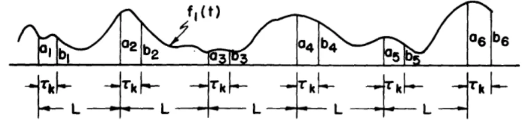
Several mechanical methods have been in use for the correlation of low-frequency random functions. At the Research Laboratory of Electronics, M. I. T., an electronic method has been developed which operates on sampling principles (ref. 14, 15). In Fig. 8 is shown a portion of a random function fl(t) whose autocorrelation curve is desired. If the function is divided into sections each of length L which is of sufficient duration so that the values al, a2, a3, ... are independent of one another, the sections
may be considered as parts of member functions of a stationary random process. For the moment assume that the random function contains no periodic component.
06 bC
Tick
1
Tk rk~- ckL L -L L _
Fig. 8 Portion of a random function showing representation of equation 53 (ref. 15)
Under these conditions the autocorrelation function on the basis of an ensemble average (49) becomes
n 11(Tk) = lim 1 j 1 a.b.
where b, b, .. is a set J J ofn (53)
where b, b, 2 b3... is a set of values of the random function each taken at a selected ,
r rl~~~~~~~~~~~~~~~~~~0
I
.% v.(t _ r
time Tk after the correspondingly numbered a-value. For a limited but large number
observations N, the approximate expression is obviously N
N(Tk = a.b.
11Tk N j=1 J j · (54)
When L is not sufficiently long to insure the independence of the sections, the expres-sion (53) may be shown to hold for the autocorrelation of a member function of a
station-ary random process. The autocorrelation function is then obtained not as an ensemble
average but a time average from sets of sampled values of the random function.
In the presence of an additive periodic component in the random function, the values of the periodic component in the different sections of Fig. 8 are no longer independent because of the definite ratio between L and the period of the periodic component.
How-ever, consideration of the random and periodic components separately leads to the con-clusion that (53) still holds provided that the ratio of the two periods is not such that the
values al, a2, a3, ... cover but a small portion of the periodic wave or a few restricted
locations on the wave.
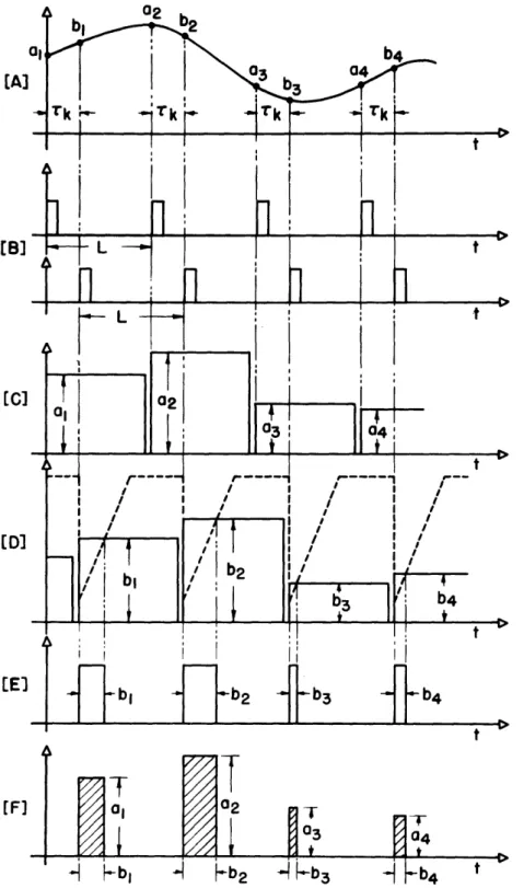
Figure 9 shows the characteristic waveforms of the electronic correlator. For the
computation of the correlation curve for the random wave (A) two sets of timing pulses (B) of period L are derived from a master oscillator, with the second set delayed by
an adjustable time Tk. By means of the first set of timing pulses the values, a, a2, a3,
.. . are selected and a boxcar wave (C) is generated so that the discretely varying heights,
are proportional to these values. A second boxcar wave (D) is similarly generated for
the values bl, b2, b3,.... A sawtooth sampling wave converts the b-values as shown in
(D) into a train of pulse-duration modulated pulses (E). A gating circuit multiplies the waveforms (C) and (E) resulting in the waveform (F) which is a series of pulses whose heights are proportional to the a-values and whose durations are proportional to the
b-values. The summation of a large number N of these pulses by an integrating
cir-cuit represents the value 11(Vk) as expressed by (54). The correlator has been
designed for complete automatic operation. The displacement Tk is varied in discrete
steps and the correlation curve is presented by an automatic recorder. The machine
performs crosscorrelation as well as autocorrelation. A sample autocorrelation
curve for filtered random noise from a Type 884 gas tube is shown in Fig. 10. 4. Characterization of a Random Process
A principal use of statistical methods in communication problems is the
charac-terization of a random process by its autocorrelation function. This characteristic
is equivalent to its power spectrum because of the reciprocal relationship through a
Fourier transformation as discussed under Section 2, Part C. Both the autocorrelation
function and the spectrum are essential in the characterization of a random process.
The situation is much like the characterization of a linear system. It is well known
that the system behavior may be expressed either as a transfer characteristic, which
-17-[A]
[e]
[C]
[D]
[El
[F]
-z
T
I
['JZ ITr H -b, H -b 2 H- -b 3 I -r a4 - ., -b4 TFig. 9 Characteristic waveforms of electronic correlator (ref. 15).
-'4 k I
"ii
E n /r n r d I-E
I ! -Y :? ' !! ! -7
I a I I I I I .Ts
Fig. 10 Autocorrelation curve for filtered noise from type 884 gas tube.
nr
wE
-UI
EJ
L
flT -'
nl F-
F
IU I
I
Fig. 11 Random flat-top wave with zero-crossings obeying the Poisson distribution.
I-t
is a function of frequency, or as a response to a unit impulse excitation, which is a
function of time. While they are determinable one from the other by a Fourier trans-
-formation, each characteristic places certain important information in much better light than the other.
The spectrum of a random wave which is specified in terms of statistics and proba-bility should be determined through autocorrelation; Fourier series and integral methods
which have been used for approximate solutions have not led to satisfactory results. As
a simple illustration consider the random wave of Fig. 11. The wave takes only the
values +E and -E volts alternately with zero-crossings obeying the Poisson distribution which states that if k is the average number of crossings per second, the probability
p(n,T) that the number of crossings in any duration T of the wave is n, is
(kn -kT
p(n,T) e (55)
Random noise which has been strongly clipped may have this waveform. Clearly Fourier
theories for periodic and aperiodic functions offer no satisfactory solution to the problem of spectrum determination. Detailed calculations are not presented here, but it is possi-ble to show that the random wave has the autocoirrelation function (ref. 4)
= E2 e k . (56)
This is a simple expression in spite of the apparent complex instantaneous behavior of
the wave. The spectrum of the random wave is readily computed by use of (44). Hence
the power density spectrum of the wave in volt2 per unit of angular frequency is
= cos e T d T
1()I
E
z
-2k|TI
E 2k
r r 4k 2 + 2 (57)
A large number of random functions under simplifying conditions may be analyzed in a similar manner for their autocorrelation functions and spectrums. A number of non-linear problems such as random noise through a rectifier have been solved (refs. 5, 9)
The experimental determination of the spectrum of a random process through the medium of autocorrelation is often more accurate and convenient than the method of
filtering. In measuring the autocorrelation function, data obtained from a long duration
enter into the computations thus ensuring an accurate measurement. For low-frequency
phenomenon mechanical correlators may be used to cover frequencies as low as a frac-tion of a cycle per second.
Because a random phenomenon reveals its statistical characteristics only after a considerable duration, correlation involves a large amount of data for accurate
determi-nation. The problem differs from the experimental spectrum analysis of a periodic wave
which yields the same data every cycle, and that of a transient which may be made to take ,,
-20-a short dur-20-ation -20-and to repe-20-at periodic-20-ally. Where-20-as -20-a filter or -20-a selective circuit will suffice in the harmonic analysis of periodic and aperiodic functions, its memory in the general case is not sufficiently long for the harmonic analysis of a random phenomenon.
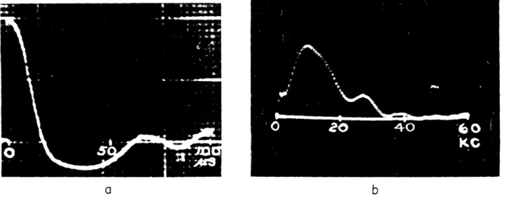
After an autocorrelation function is obtained the transformation required for produc-ing the power spectrum may be performed by machine. For illustration an autocorrela-tion curve of filtered noise from a Type 884 gas tube which has been computed by the
electronic correlator is shown in Fig. 12a (ref. 11). The power density spectrum of
the noise given in Fig. 12b is obtained by a cosine transformation by means of the high-speed differential analyzer developed at the Research Laboratory of Electronics, M. I. T.
a
b
Fig. 12a Autocorrelation curve of fil- Fig. 12b Power density spectrum of the tered random noise from Type 884 gas noise determined by differential analyzer. tube measured by correlator.
5. Separation of Periodic and Random Components
A random process may have a hidden periodic component and in many communication problems it is important to separate the random and periodic components. Since random
and periodic phenomena behave differently under autocorrelation, each in a characteristic manner, autocorrelation is an effective tool in the problem of separation. Autocorrela-tion of a periodic funcAutocorrela-tion produces another periodic funcAutocorrela-tion of the same fundamental frequency while that of a random function results in a maximum value when the
displace-ment is zero, which represents the function's mean square value, and the square of the mean value as the displacement tends to infinity. These different properties make it possible to resolve the autocorrelation function into two components.
By way of illustration, consider the pulse-duration modulated wave of Fig. 13. This wave has a periodic component although it is not apparent, by examination of its
l
l
n
TE
FH
n
-X1- A Pi -A .A + A ' A ---A--*- t Fig. 13 A pulse-duration modulated wave.
wave form, as far as the exact amount is concerned. The leading edges of the pulses occur at regular intervals. For reasons of simplicity let the intervals be ZA, and the pulse duration x vary randomly with a uniform distribution between the limits (0, A), and let the durations be independent of each other. Based upon these assumptions, it is possible to show that the autocorrelation function of the pulse-duration modulated wave has the form shown in Fig. 14. The curve has the highest peak at the center and peaks
a 1(T)
-5A -4A -3A -2A -A 0 A 2A 3 4A 5A r Fig. 14 Autocorrelation function of the pulse-duration modulated wave of Fig. 13.
of the same shape at periodic intervals of 2A. Clearly this curve may be resolved into two parts, one periodic and one aperiodic as Fig. 15 shows. The aperiodic component has the expression
E
2 3
E (A- IT)3 -A< <
(~' T)] - 12 A
ll(T)] random (58)
0 elsewhere
which is the autocorrelation function of the random component of the pulse-duration modulated wave. By a Fourier transformation the power density spectrum of the random component wave is found to be
2 (sin A- - 2
[ 11()] random 4ir(AW )2
L
1 A (59)The autocorrelation function of the hidden periodic component wave is determined com-pletely when the expression for a half cycle of the function is known. The expression is
E 2 E 3
[11() periodic 4A2 [14 (a2 (A T - T)
- 3(A - T)3 0 < T< (60)
from which the power spectrum of the periodic component wave is readily computed by application of (12).
[11 (r)] PERIODIC
, -. . - : Fig. 15 Periodic and aperiodic
-D -so - -s - n U Li n a 4 Do T components of the autocorrelation
| [ l( )] RANDOM function of Fig. 14.
-A 0 A T
The method of analysis is applicable to other types of pulse-modulated waves
(ref. 10). When the degree of dependence between pulses is appreciable, calculations
increase in complexity so that it becomes necessary to obtain the autocorrelation
curve experimentally. If the autocorrelation curve maintains its periodic behavior
as T tends to large values the method described here should be effective in the
sepa-ration of periodic and random component waves which are not easily distinguished in a random process.
6. Filtering and Prediction
In filtering, the objective is to extract the desired message from a mixture of
message and noise. Stated in more general terms, the problem is the recovery of
a random process which has been corrupted by another random process. The recovery
is to be done by a linear system which has been designed in accordance with the
statis-tical characteristics of the stationary random processes involved. The filter operates
upon the past values of the corrupted random process as it progresses in time in such a way that the instantaneous output of the filter is the best approximate instantaneous
value of the desired random process. The meaning of the term "best" depends upon
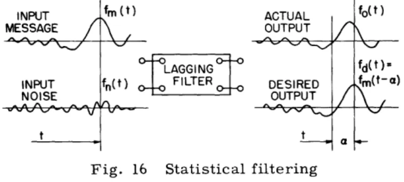
the particular measure of error and the criterion in the formulation of the filter problem. In the statistical filter theory of Wiener (ref. 2), the input to the filter consists of
an additive mixture of message and noise as indicated in Fig. 16. The desired ideal
out-put is the message itself with possibly a preassigned fixed delay time . Since perfect
recovery is a physical impossibility, the instantaneous error is the difference between the actual output fo(t) and the desired message with a lag fm(t - a). A measure of error
INPUT MESSAGE - I , INPUT NOISE t fm (t) .... .A1. IL.. /i,,4 *9IUIAL OUTPUT k
~tft~t-LAGGING fn(t) - FILTER 116- A DESIRED OUTPUT ti
L
a f (t) \-fd(t)= fm(t- a)Fig. 16 Statistical filtering
which is relatively simple to manage in the subsequent analytical work, and which is meaningful in a number of physical situations is the mean square error. The expres-sion for the mean square error is
T
im
(t - fm(t - a) 2dt. (61)
T- lim 2T i [fo( ) m ]
The criterion in the design of a filter should therefore be that the mean square error
of calculus of variations it is possible to show that if .ii(T) is the input autocorrelation
function and im(T) the input and message crosscorrelation function, the response characteristic h(t) of the optimum filter to a unit-impulse excitation must satisfy the condition that
~im( T- ) = h(Ca)bii(T - )dcr, for T 0 (62)
-00
This integral equation is of the Wiener-Hopf type, the explicit solution of which for the Fourier transform of h(t) in terms of the Fourier transforms of ii(T) and bim(T) has been achieved. Although the analytical work is by no means simple, it is possible to proceed from the given autocorrelation and crosscorrelation functions to obtain the optimum filter characteristic for the practical construction of a filter consisting of linear passive elements and possibly amplifiers.
In classical filter theory the concepts are those belonging to periodic phenomena. The idea of the division of the spectrum into pass bands and attenuation bands is basic. When the messages and noise involved in a filter problem have spectrums which are essentially not overlapping, the classical filter is simple and effective. However, in the general case where the best separation of two or more random processes by means of linear systems is required, classical theory fails to provide a satisfactory solution.
The difficulty in classical theory in this respect is a fundamental one.
An interesting and important problem in the theory of random processes is that of prediction. It is remarkable that, on the basis of statistical concepts, filtering and prediction are closely related problems. For simplicity consider prediction in the
absence of noise. The desired output in a linear predictor is the input itself except for an advance in the time of occurrence. Since exact prediction for a random process
even in the absence of noise is impossible, a measure of error and a design criterion are necessary as in the case of filtering. If f(t) is the input message, f(t) the actual output, and a the preassigned prediction time, the mean square error is clearly
T
T -T fo(t) - f(t+ a)] 2dt (63)
-T
For optimum prediction by a linear system, the predictor characteristic h(t) as a time response to unit-impulse excitation must satisfy the integral equation
00
~mm(T + a) = h()jMM( - Co)dC for T 0 (64)
-00
which is similar to (62). Here mm( T) is the autocorrelation function of the message. The theory of the optimum linear statistical predictor has been demonstrated in the Laboratory (ref. 16). The block diagram for the demonstration is given in Fig. 17. Random noise from a Type 6D4 gas tube is used as the message to be predicted. The filter shown is a simple R-L-C parallel circuit for shaping the spectrum of the noise.
Fig. 17 Block diagram for demonstration of prediction.
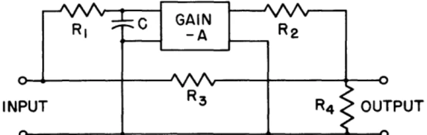
Fig. 18 Basic circuit diagram of predictor for demonstration (ref. 16).
When designed in accordance with statistical theory the predictor has the simple basic form shown in the diagram of Fig. 18. The comparison device of Fig. 17 is a high-speed
camera which records continuously the input and output random waves with the aid of a two-beam oscilloscope. This instantaneous recording permits the comparison of actual and predicted values of the random noise. Sample records are shown in Fig. 19 for three prediction times. Inspection of these results shows that a close agreement between actual and predicted values has been obtained.
7. Use of Random Noise in System Characteristic Determination
Of fundamental importance in the analysis of linear systems is the characterization of the system. Because of the applicability of the principle of superposition, a linear system is characterized either by a time response h(t) to a unit-impulse excitation (a unit-step function may be used instead), or by amplitude and phase spectrums of the transfer ratio H(w) when the driving force is in steady-state sinusoidal form. The functions h(t) and H(w) are known to be related by a Fourier transformation. These characteristics furnish basic information concerning the behavior of the system and are therefore useful directly or indirectly in a problem.
A third method for obtaining the system characteristic involves the use of random noise instead of the unit impulse or the steady-state sinusoid. This method has some advantages.
For the development of the theory, consider the linear system shown in Fig. 20. The input is a stationary random function f(t) and the output is f (t). The system has
1 0
the time response h(t) to a unit-impulse excitation or the corresponding complex spectrum H(w). The crosscorrelation function between the input and output of the
system is: ''
o bl a) .-I 0 -U)2 O,--a) 4 0 0O 0O 0 - O4 o U) . 0 -'-4 .-C) O U) -o H a ^4 r
T
io (T) = lim 1 tf(t (65)
T+ oo 2 -T )f(t)d Since the system is linear, the superposition integral
f(t) = i h(a)fi(t- )do (66)
-00
holds for the random functions fi(t) and fo(t). The use of this integral in (65) leads to
For the type of random functions under consideration, a change in the order of integra-tion is permissible, so that
co
T
bio (T) = h(o)d limr 1 fi(t)fi(t + - )dt (68)
1O T* T
The limit integral appearing in the equation is recognized as the autocorrelation function
ii(T - ). When this symbol is used (68) becomes
-o
4.(
) = h(cr)ii(r - c)d0 . (69)This is a fundamental equation for a linear system with random input and output functions. The equation is a convolution integral, exactly the same in form as the well-known
super-position integral (66). The integral (69) states that the input-output crosscorrelation
function of a linear system, which is under excitation by a stationary random function, is the convolution of the system response to a unit-impulse excitation and the input
auto-correlation function. Since
4ji
is an even function it is possible to write (69) in the formof a correlation function by changing ii(T - ) to ii(c- T)
fi(t ) = h(l - f(t
A
H (w)
Fig. 20 A linear system with
a random function as input.
The expression of the integral (69) in the frequency domain can readily be done by
a Fourier transformation. This transformation leads to the result that
tio
()
= H(w) iii() (70)in which io() is the cross power density spectrum between input and output, and cii(o)
is the input power density spectrum. This basic equation shows clearly that
is exactly the phase spectrum of the cross power density spectrum.
When white noise is considered, ii in (69) takes the form of an impulse. If a unit
impulse is assumed for this function the integral simplifies to
bio(T ) = h(T) . (71)
This is an interesting result. It states that the time response of a linear system to a unit-impulse excitation has a form identical to the crosscorrelation function between
the input and output of the system when the input is a white noise. The corresponding
statement of the result in the frequency domain according to (70) is that
~io(O) = H(w) (72)
if Hii(w) has a uniform spectrum of unity.
Physically a white noise is taken to mean a noise whose spectrum remains essen-tially constant over a band of frequencies which is considerably wider than the effective band of the system under test. Experimental results illustrating the theory are shown
in Fig. 21a and b. A simple resonant circuit with a time response to a unit impulse
of the form shown in Fig. 21a is subjected to a white noise excitation. A crosscorrela-tion curve is then obtained by the digital electronic correlator which has been developed
recently at the Research Laboratory of Electronics, M. I. T. (ref. 14). The curve is
shown in Fig. 21b. This experiment verifies the equation (71).
A significant advantage of this method is that internal or external random noise which may be present while measurements are made does not appreciably affect the
results. The reason is that these extraneous noise sources are incoherent with the
input noise so that crosscorrelation between them theoretically results in either a
con-stant or zero. This conclusion has been experimentally verified.
The method and technique of determining system characteristics by application of random noise based on the fundamental equation (69) have other possible significant applications.
8. Detection of Repetitive Signal in Random Noise
A problem of considerable importance in communication theory is the detection of a repetitive signal which has been masked by random noise. In a radar system, or in other systems which operate on the principle of echoes, the improvement of signal-to-noise ratio is such a problem.
In the discussion on the separation of periodic and random components of a random
process the method of correlation is shown to be effective. The method is clearly
applicable to the present problem since the basic elements involved and the require-ments are similar though not identical.
Consider (ref. 15) an additive mixture of a repetitive signal S(t) and a random noise N(t) which is written as
r
-· K if.*
;~
-i'
I
---~~
5 I .4 Cd oc v ; t h "·:, : . -, f X 0). c-I-Y a' '. V1If
+
:z
t * SoS t -I~ f, 0 E $ a o (D NW) 0)QISk .4-bfO CdoO~ $HIQ * W D, i i j !f· al , ·;tI:`rt· ·---F -i; rij'·
i ·. ,·, g & ::" ; :ii" :iitl"tB 811
i· J:i·r ;· II. .·.· ; f t·;6ii. "I i ; . ··.. ....; Cqr;,Et, """ 'J B· ij · r !..·E· il e*· ·! t .Il-i-T*-- -L e* i
a---
1
·- iI-I1 I zr IzI .i __ _- 1 . 1 5fl(t) = S(t) + N(t) The autocorrelation function of fl(t) is
T
l(=) =l 2 (t) + N(t)] [S(t + ) + N(t + T) dt
-T
= qbSS(T) + 4NN(T) + SN(T) + qNS(T) (74)
The first two terms are the autocorrelation functions of the signal and noise respectively
and the remaining terms are their crosscorrelation functions. Since signal and noise
are incoherent, their crosscorrelation is zero if the mean value of either component is
taken to be zero. The conclusion is that the autocorrelation function of the sum of signal
and noise is the sum of the individual autocorrelation functions. This result is
graphi-cally illustrated in Fig. 22 for a sinusoidal signal. Since the autocorrelation of random noise drops to a final value, whereas that of the repetitive signal remains repetitive, it
is clear that in the region of T where noise autocorrelation has practically reached a
final value a periodic variation is evidence that a repetitive signal is present.
0 I(T)
I-
n
Fig. 22 Autocorrelation function of
sinusoid plus random noise. Dotted curve is component due to noise (ref. 15).
Improvement in signal-to-noise ratio is dependent upon the length of time of
observa-tion. When detection is carried out by the electronic correlator, the random variable
from which samples are taken is
'
= [S(t) + N(t)]
[S(t
+ T') + N(t + TS(t)S(t + T ) + N(t) N(t + T1) + S(t) N(t + T') + N(t) S(t + T') (75)
in which T' is the displacement whose lower limit should be in the neighborhood of the
value at which qNN(T) is essentially constant. Since the correlator computes the output
graph as a series of discrete values, each of which is the result of a large number of samples, the dispersion of these points about the ideal mean curve is a measure of
output "noise". This noise is obviously not random noise in the ordinary sense but an
(73)
error due to the limited number of observations made for each value of the autocorrela-tion curve. In other words the noise is a dispersion of a set of sample means about a limit which they approach as the sample size increases indefinitely. In calcuating the output noise the theory of sample means is applied. For a sinusoidal signal, the corre-lator output signal-to-noise ratio for autocorrelation is
R = 10 log, n db (76)
oa= 10 0 1 + 4 2 + 2 4
in which n is the number of sample products which the correlator takes for a point on the output curve, and pi is the rms noise-to-signal ratio at the input. A curve of this equation when n = 60, 000 is drawn in Fig. 23. For example, when the input signal-to-noise ratio is -20 db, the ratio at the correlator output is +4 db giving a total gain of 24 db. 2 Q t
Z
2 ti W 52 z 0 a. 0 4C 30 20 10 -10 -20 -30 -An 15 10 5 0 -5 -10 -15 -20 -25 -30 -35 -40INPUT SIGNAL- TO- NOISE RATIO IN DB
Fig. 23 Signal-to-noise ratio gain in detection of sine wave in random noise by autocorrelation and crosscorrelation (ref. 15).
The theory and calculations have been varified by experiment. In Fig. 24 are shown correlator output graphs for an 8-kc sine wave plus random noise from a Type 884 gas tube at several ratios at the input. The relatively flat portions of the graphs are ob-tained when noise alone is at the input. The presence of a sine wave is clearly in-dicated by a sinusoidal variation.
When the repetition period of the signal is known a further gain may be had by ap-plication of crosscorrelation. For this purpose a local signal of the same repetition rate is generated. The theoretical crosscorrelation function between the local signal and the corrupted signal is
12( T ) = lim 2T
[
S(t) + N(t) S2(t + T)dt S l (T) + NS (T) (77) I I60,000 n 60,0001 1
0-%%1 I
'__
\_1
C110
-_
11,19SCr~"
I I"';</O* I.
II
I I I
I
;J%; e
=-\7-X
I-4 0 -4 -4 0 .-4 a)