Anisotropic Perfectly Matched Layers for Elastic Waves in Cartesian and Curvilinear Coordinates

Anisotropic Perfectly Matched Layers for Elastic Waves in

Cartesian and Curvilinear Coordinates

Yibing Zheng and Xiaojun Huang

Earth Resources Laboratory

Dept. of Earth, Atmospheric, and Planetary Sciences

Massachusetts Institute of Technology

Cambridge, MA 02139

Abstract

We develop new numerical anisotropic perfectly matched layer (PML) boundaries for elastic waves in Cartesian, cylindrical and spherical coordinate systems. The elasticity tensor of this absorbing boundary is chosen to be anisotropic and complex so that waves from the computational domain are attenuated in the boundary layer without reflection. The new PMLs are easy to formulate for both isotropic and anisotropic solid media. They utilize fewer unknowns in a general three-dimensional problem than the existing elastic wave PMLs using the field splitting scheme. Moreover, it can be implemented directly to the finite element method (FEM), as well as the finite difference time domain (FDTD) method. The high efficiency of these PMLs is illustrated by some numerical samples in FEM.

1

Introduction

In numerical computation of wave problems, absorbing boundary conditions (ABCs) are widely used to truncate an unbounded medium into a finite domain and to eliminate reflections from numerical boundaries. Among all kinds of ABCs, the perfectly matched layer (PML) absorbing boundary performs more efficiently and more accurately than most traditional or differential equation-based absorbing boundaries (Shlager and Schneider, 1998). Berenger (1994) first created a true PML for electromagnetic (EM) waves in the finite difference time domain (FDTD) method. This numerical absorbing boundary is a layer of an artificial material that is placed around the computational domain. It is designed to absorb thoroughly any incident wave of any frequency at any incident angle without reflection. The absorbing layer is only a few lattice cells thick. Therefore, it has very strong attenuation so that waves are absorbed quickly in a very short distance. In Berenger’s initial work of the PMLs for EM waves in the FDTD method, a split-field formulation of Maxwell’s equations is derived, and each field component is split into two subcomponents in a two-dimensional case (Berenger, 1994). Following Berenger’s work, Chew and Weedon (1994) introduced the idea of complex coordinate stretching of Maxwell’s equations to obtain the same PML. This idea made the formulation of the PML much more straightforward and convenient.

The field splitting method results in an increase in the number of variables. In a three-dimensional prob-lem, the number of variables may increase three times. Moreover, the split-field formulation of Maxwell’s equations is difficult to apply to the finite element method (FEM). Sacks et al. (1995) developed an anisotropic PML for EM waves, which does not require field splitting. It can be easily implemented in the FEM, as well as in the FDTD method. In this type of PML, entries of both electric and magnetic permittivity tensors are modified to have strong attenuation, yet the layer still perfectly matches the com-putational domain. This absorptive material must be anisotropic. The anisotropic PML introduces some physical understanding, although this material is created artificially.

The PML formulation was extended from Cartesian coordinates to curvilinear coordinates by various efforts. Kuzuoglu and Mittra (1997) directly applied Sacks’s PML to cylindrical coordinates. However, such application neglected a geometric factor, resulting in a quasi-PML, which could only get near zero reflection when the PML is placed far enough away from the symmetric axis. Furthermore, this PML may cause

significant fault results in stationary or eigenvalue problems. Maloney et al. (1997) successfully derived the PML in cylindrical coordinates for EM waves using a graphical approach. Teixeira and Chew (1997a) applied the complex coordinate stretching method, derived the PMLs for EM waves for the FDTD method in both cylindrical and spherical grids, and then extended them to anisotropic PMLs (Teixeira and Chew, 1997b).

The PML technique has also been used to solve acoustic and elastic wave propagation problems. Fur-thermore, it has strong applications in acoustic well logging and seismic wave survey, etc. Earlier studies of the elastic wave PML are concentrated mostly on Cartesian coordinates (Chew and Liu, 1996; Hastings et al., 1996). Liu (1999) formulated the PMLs for elastic waves in cylindrical and spherical coordinates based on an improved complex coordinate stretching and field splitting for the FDTD method. Liu’s formu-lations have shown good results in time domain problems. Normally, by using the field splitting method, the PML for elastic waves has 27 independent unknowns for a general three-dimensional problem (9 for velocity components and 18 for stress components), three times the original 9 variables in ordinary linear elasticity governing equations. This also requires 27 independent equations to solve the problem. If the computational domain is isotropic, the number of unknowns can be reduced to 24, or at least 18, when the normal stress components of the sources are identical (Liu, 1999). Besides the large number of variables, it is difficult to implement the split-field PMLs using the finite element method.

Although the anisotropic PMLs for EM waves have been developed without the field splitting, the study of anisotropic PMLs for elastic waves has not yet been found. This raises the question of whether the anisotropic PML for elastic waves exists or not. Here we prove its existence and develop such anisotropic PMLs for elastic waves in Cartesian, cylindrical and spherical coordinates. The formulation of these new PMLs avoids the tedious work of field splitting and is easy to generate, especially for anisotropic media. More importantly these PMLs can be used in the FEM directly, and in the FDTD method as well. In the frequency domain FEM, we use only three displacement variables whether the computational domain is isotropic or anisotropic. For stable implementation in the FDTD, besides the basic 12 variables (3 velocity variables and 9 stress variables), extra interim variables are used so that the total number of unknowns are 21, less than 27 in the field splitting formulation. A decrease in numbers of variables and equations can reduce the amount of computer memory and computing time. Numerical results for some special cases are presented using the finite element method to illustrate the effectiveness of these anisotropic PMLs.

2

Anisotropic PML for Elastic Waves

2.1

Cartesian coordinates

The propagation of linear elastic waves in any solid material is governed by the equation of motion and the generalized Hooke’s law. They are written symbolically in vector and tensor form as

ρ∂ 2_u

∂t2 = ∇ · T, (1)

T= C : S. (2)

Here u = [ux, uy, uz]T is the displacement vector, and T is the stress tensor,

T=       Txx Txy Txz Tyx Tyy Tyz Tzx Tzy Tzz       , (3)

where Tij represents the stress acting on the coordinate plane i and having the direction along the j axis. C is the fourth order elasticity tensor, whose elements are cijkl (i, j, k, l = x, y, z). S is the strain tensor, which

is related to the displacement vector by

S=1

2(∇u + (∇u)

T_{). (4)}

The tensor of the displacement gradient, ∇u, is defined as

∇u =       ux,x uy,x uz,x ux,y uy,y uz,y ux,z uy,z uz,z       , (5)

where ui,j= ∂ui/∂j. Therefore, explicit expressions of Eqs. (1) and (2) in Cartesian coordinates read

ρ∂ 2_u j ∂t2 = Tij,i, (6) Tij= cijklSkl= 1 2cijkl(uk,l+ ul,k), (7) where the summation convention is applied.

The elasticity tensor of an isotropic solid has only two independent constants. The general Hooke’s law can be written as

T= λI(∇ · u) + µ(∇u + (∇u)T_{), (8)} where λ and µ are Lam´e constants, and I is the second order unit tensor.

In real solids, body torques are always negligible, so that the stress tensor is symmetric, namely, Tij = Tji. Therefore, the theory of linear elasticity only needs to utilize six stress variables. By using abbreviated subscripts, the stress variables can be written as a six-element single-column matrix. The generalized Hooke’s law, Eq. (7), is then simplified to six equations. The strain tensor S by definition is symmetric and can be also represented by six variables. As a result, the elasticity tensor C becomes a 6-by-6 matrix.

To derive the PML formulation for elastic waves using the FDTD method, the complex coordinate stretching method is applied to these governing equations (Chew and Weedon, 1994; Chew and Liu, 1996). The complex coordinate variables are defined as

˜ xi= x0i + Z xi x0 i εi(x0)dx0, (i = 1, 2, 3), (9)

where εi is a complex number. Notice that ∂/∂ ˜xi= (1/εi)∂/∂xi. The region xi< x0i is the computational domain, where the true wave solutions are wanted. The absorbing boundary layer is the area where xi> x0i, and the boundary interface is thus placed at xi= x0i. In the absorbing layer, the complex coordinate stretch-ing method replaces the original coordinate variables xiwith the complex coordinate variables ˜xiin both the equation of motion and Hooke’s law, Eqs. (1) and (2), respectively. Because εiis complex and its imaginary part is related to the wave attenuation coefficient, waves in the boundary layer are attenuated. Furthermore, since the new equations in the complex stretched coordinates have the exact forms as those in the original non-stretched coordinates, waves passing through the interface will not result in any reflection (Chew and Liu, 1996). The absorbing boundary region becomes a layer that perfectly matches the computational do-main. When this PML is used in the FDTD method, both the displacement and stress variables need to be split, and that causes the increase of the number of variables (Liu, 1999).

The formulation of our anisotropic PML for elastic waves is different from that of the PML using the field splitting method, although the derivations of both PMLs start from the complex coordinate stretching scheme. The anisotropic PML formulation requires that the waves in the PML are still governed by the equation of motion and Hooke’s law, with the divergence and gradient expressed in the non-stretched coor-dinates. That means the properties of the material can be modified, but not the physical principles behind the governing equations. We will see later that in this artificial anisotropic absorptive material, the stress tensor is no longer symmetric. Therefore, we have to include all 9 stress variables in Eq. (1), and cannot use

the abbreviated notations. Tij and Tjishould be distinguished when i 6= j. The strain tensor will no longer be used. Instead, only the tensor of the displacement gradient, ∇u, is used in Eq. (2). Due to the symmetry of the elasticity tensor of real solid materials, cijkl = cijlk, we can rewrite Eq. (7) in the form of

Tij= cijklul,k, (10)

which gives us the same Tij. In vector and tensor form, this alternative Hooke’s law becomes

T= C : ∇u, (11)

without the strain tensor. Combining Eqs. (1) and (11), we obtain the elastic wave equation, ρ∂

2_u

∂t2 = ∇ · C : ∇u. (12)

Applying the complex coordinate stretching to the equation of motion, Eq. (1) of an originally isotropic region, we get the explicit equations in the absorbing boundary layer.

−ρω2ux= 1 εx ∂Txx ∂x + 1 εy ∂Tyx ∂y + 1 εz ∂Tzx ∂z , (13) −ρω2uy= 1 εx ∂Txy ∂x + 1 εy ∂Tyy ∂y + 1 εz ∂Tzy ∂z , (14) −ρω2uz= 1 εx ∂Txz ∂x + 1 εy ∂Tyz ∂y + 1 εz ∂Tzz ∂z . (15)

Here, a new set of stress variables is defined as ˜ Txx= εyεzTxx, T˜xy = εyεzTxy, T˜xz = εyεzTxz, (16) ˜ Tyx= εzεxTyx, T˜yy= εzεxTyy, T˜yz= εzεxTyz, (17) ˜ Tzx= εxεyTzx, T˜zy= εxεyTzy, T˜zz= εxεyTzz. (18) Or in tensor form, ˜ T=       εyεz 0 0 0 εzεx 0 0 0 εxεy       T= εxεyεzΛ· T, (19)

where Λ is a second order tensor as

Λ=       1/εx 0 0 0 1/εy 0 0 0 1/εz       . (20)

We may call it the coordinate stretching tensor. With these new stress variables, we can reconstruct the equation of motion and rewrite it in the form of the divergence of the stress in the non-stretched coordinates, as

−ρω2εxεyεzu= ∇ · ˜T. (21) After the complex coordinate stretching and the substitution of Eq. (19) into Eq. (11), the Hooke’s law is

transformed to ˜ Txx= (λ + 2µ) εyεz εx ∂ux ∂x + λεz ∂uy ∂y + λεy ∂uz ∂z , (22) ˜ Txy = µεz ∂ux ∂y + µ εyεz εx ∂uy ∂x , (23) ˜ Txz = µεy ∂ux ∂z + µ εyεz εx ∂uz ∂x, (24) ˜ Tyx = µεz ∂uy ∂x + µ εzεx εy ∂ux ∂y , (25) ˜ Tyy = λεz ∂ux ∂x + (λ + 2µ) εzεx εy ∂uy ∂y + λεx ∂uz ∂z , (26) ˜ Tyz = µεx ∂uy ∂z + µ εzεx εy ∂uz ∂y , (27) ˜ Tzx= µεy ∂uz ∂x + µ εxεy εz ∂ux ∂z , (28) ˜ Tzy = µεx ∂uz ∂y + µ εxεy εz ∂uy ∂z , (29) ˜ Tzz = λεy ∂ux ∂x + λεx ∂uy ∂y + (λ + 2µ) εxεy εz ∂uz ∂z . (30)

These equations can be expressed as a generalized Hooke’s law using a new effective elasticity tensor, ˜C, ˜

T= ˜C: ∇u, (31)

where the entries of ˜Care

˜

cijkl= cijkl εxεyεz

εiεk

, (i, j, k, l = x, y, z). (32) Eqs. (21) and (31) are the equation of motion and Hooke’s law in the absorptive medium expressed in the non-stretched coordinates.

We now show that across the boundary interface the stress T in the computational domain continues to ˜

T, satisfying the physical boundary condition. Suppose this two-dimensional interface is located at z = 0. The half-space where z < 0 is the computational domain, and the other half-space is the absorptive medium. The complex coordinate stretching is performed only in the z direction. Therefore, εx= εy = 1, and εz6= 1.

˜ T=       εz 0 0 0 εz 0 0 0 1       T=       εzTxx εzTxy εzTxz εzTyx εzTyy εzTyz Tzx Tzy Tzz       . (33)

Note that ˜Tzj = Tzj, (j = x, y, z), which means that in the absorptive medium, the components of ˜Ton the plane perpendicular to the z axis are the same as those of T in the computational domain. This satisfies the physical interface continuity condition that the stresses on the interface on both sides should be the same. Therefore, we can replace ˜Twith T in Eqs. (21) and (31), and get the governing equations in the absorptive medium as

−ρω2εxεyεzu= ∇ · T, (34)

T= ˜C: ∇u. (35)

Its wave equation in the frequency domain turns out to be −ρω2_ε

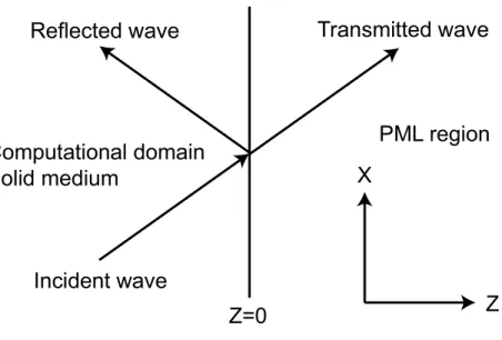
Figure 1: Elastic wave reflection and transmission at a boundary

To prove that this absorptive medium behaves as a perfectly matched layer, consider an incident plane wave and the areas near the interface in both half spaces are homogeneous. Without loss of generality, suppose that the plane of incidence coincides with the xz plane, so that ∂/∂y = 0, as shown in Figure 1.

Consider an arbitrarily polarized plane elastic wave u = u0ei(ωt−ik

a

xx−ikzaz)propagating in the absorptive

medium governed by Eqs. (34) and (35), where the superscript a denotes the absorptive medium. The Christoffel equation (Auld, 1973) associated with the wave equation, Eq. (36), appears in the form

       εz(kax)2(λ + 2µ) + (kaz)2 µ εz 0 ka xkza(λ + µ) 0 εz(kax)2µ + (kaz)2 µ εz 0 ka xkza(λ + µ) 0 εz(kax)2µ + (kza)2 λ + 2µ εz              ux uy uz       = ρω2εz       ux uy uz       . (37)

The dispersion relations for the absorptive medium are obtained by setting the characteristic determinant of the Christoffel equation to zero. Solving for ka

xand kza, we find that there are four eigenvalue solutions. (kxa)2+ (kza)2/ε2z= ρω2/(λ + 2µ) = ω2/Vp2, (38)

(kxa)2+ (kza)2/ε2z= ρω2/µ = ω2/Vs2, (39) where Vp =p(λ + 2µ)/ρ and Vs=pµ/ρ are the compressional and shear wave velocities in the isotropic medium. Eq. (38) is the dispersion relation for a quasi-compressional wave in the absorptive medium, and Eq. (39) is for two quasi-shear waves.

Now consider the case of the incident of a compressional or shear wave (P or S wave) from the isotropic computational medium, respectively. The non-slip boundary conditions at the interface require that all of the displacement components, ux, uy and uzare continuous, as well as the stress components acting on the interface, Tzx, Tzy and Tzz. In general, the stress continuity condition requires the continuity of ˆn· T, where ˆ

nis the unit normal vector of the interface.

2.1.1 P _wave

The incident P wave in the isotropic computational medium can be expressed as

u= u0kpei(ωt−kp·x)= u0kpei(ωt−kpxx−kpzz), (40) where the compressional wave number kp = kpxˆx+ kpzˆz, and ˆx and ˆzare the unit vectors of the x and z axes. We also have the wave number relation, k2

px+ k2pz = ω2/Vp2. This incident wave results in only one quasi-longitudinal wave in the absorptive medium as

ua= u0kpei(ωt−k

a

xx−kazz)= u

0kpei(ωt−kpxx−εzkpzz), (41) which satisfies the continuity boundary conditions thoroughly. Here ka

x = kpx and kza = εzkpz, which agree with the dispersion relation of Eq. (38) for the quasi-compressional wave. Since the incident and the transmitted waves have already met the displacement and stress continuity condition at the interface, no reflection wave exists.

2.1.2 S _wave

If an S wave is incident from the isotropic domain, it has the form

u= (us× ks)ei(ωt−ks·x)= (us× ks)ei(ωt−ksxx−kszz), (42) where the shear wave number ks = ksxˆx+ kszˆz, and ksx2 + ksz2 = ω2/Vs2. us is a vector that is not parallel to ks. In this case, only one quasi-shear wave is transmitted into the absorptive medium, which is

ua = (us× ks)ei(ωt−k

a xx−k

a

zz)= (u_s× k_s)ei(ωt−ksxx−εzkszz)_{. (43)}

Both the stress and velocity continuity conditions are satisfied. ka

x= ksxand kaz= εzksz, which are consistent with the dispersion relation of Eq. (39) for the quasi-shear wave. Again there is no reflection wave or other transmitted wave.

Therefore, the absorptive medium governing by Eqs. (34) and (35) is a perfectly matched absorbing layer. Although all the demonstrations above are for an isotropic medium, this anisotropic PML boundary is suitable for any anisotropic computational domain as well. The complex coordinate stretching method does not limit itself to an isotropic medium. We can apply the stress transformation, Eq. (19), and the coordinate stretching tensor Λ in Eq. (20) to any kind of medium. We then get the equation of motion that is the same as Eq. (34). Hooke’s law takes the form

T= εxεyεzΛ· C : (Λ · ∇u). (44)

Rewriting Eq. (44) using a new effective elasticity tensor ˜C, we obtain the same form as Eq. (35), and the elements of ˜C are represented by Eq. (32). To this end we generalized the anisotropic PML governed by Eq. (34) and (35) to any kind of computational media. The number of unknowns in this PML formulation is always 12 (3 displacement components and 9 stress variables).

2.2

Cylindrical coordinates

In cylindrical coordinates (r, φ, z), the governing equations of linear elastic waves are the same as Eqs. (1) and (11). The displacement vector and the stress tensor are

T=       Trr Trφ Trz Tφr Tφφ Tφz Tzr Tzφ Tzz       . (46)

As in Cartesian coordinates, we distinguish between Tij and Tji, (i, j = r, φ, z and i 6= j). The expressions of ∇·T and ∇u are more complicated here than those in Cartesian coordinates. Expressed explicitly, equations of motion are −ρω2ur= 1 r ∂ ∂r(rTrr) + 1 r ∂Tφr ∂φ − Tφφ r + ∂Tzr ∂z , (47) −ρω2uφ= 1 r ∂ ∂r(rTrφ) + Tφr r + 1 r ∂Tφφ ∂φ + ∂Tzφ ∂z , (48) −ρω2uz= 1 r ∂ ∂r(rTrz) + 1 r ∂Tφz ∂φ + ∂Tzz ∂z . (49)

The tensor of displacement gradient has the form

∇u =          ∂ur ∂r ∂uφ ∂r ∂uz ∂r 1 r ∂ur ∂φ − uφ r ur r + 1 r ∂uφ ∂φ 1 r ∂uz ∂φ ∂ur ∂z ∂uφ ∂z ∂uz ∂z          . (50)

In cylindrical coordinates, PMLs may be placed along all three directions. We introduce the complex stretching coordinate transformation similar to that in Cartesian coordinates,

˜ r = r0+ Z r r0 εr(r0)dr0, (51) ˜ φ = φ0+ Z φ φ0 ε0 φ(φ 0 )dφ0 , (52) ˜ z = z0+ Z z z0 εz(z0)dz0. (53) Note that ∂ˆr/∂ ˜φ = ˆΦ/ε0 φ and ∂ ˆΦ/∂ ˜φ = −ˆr/ε 0

φ, where ˆr and ˆΦ are the unit vectors of r and φ directions. The prime sign is purposely added to the stretching number along the φ direction, ε0

φ.

Applying this coordinate stretching to Eqs. (47) to (49), we get equations of motion in the stretched form as −ρω2ur= 1 ˜ rεr ∂ ∂r(˜rTrr) + 1 ˜ rε0 φ ∂Tφr ∂φ − Tφφ ˜ rε0 φ + 1 εz ∂Tzr ∂z , (54) −ρω2uφ= 1 ˜ rεr ∂ ∂r(˜rTrφ) + Tφr ˜ rε0 φ + 1 ˜ rε0 φ ∂Tφφ ∂φ + 1 εz ∂Tzφ ∂z , (55) −ρω2uz= 1 ˜ rεr ∂ ∂r(˜rTrz) + 1 ˜ rε0 φ ∂Tφz ∂φ + 1 εz ∂Tzz ∂z . (56)

Again we can transform the original T into a new set of stress variables ˜Tby

˜ T=       εzε0φ ˜ r r 0 0 0 εrεz 0 0 0 εrε0φ ˜ r r       T= εrεzε0φ ˜ r rΛ· T, (57)

where Λ is the coordinate stretching tensor, Λ=       1/εr 0 0 0 r/(˜rε0 φ) 0 0 0 1/εz       . (58)

Therefore, the equation of motion will include the divergence of the new stress tensor in the non-stretched coordinates.

−ρω2εrεzε0φ ˜ r

ru= ∇ · ˜T. (59)

The tensor of displacement gradient in the stretched coordinates becomes ˜

∇u = Λ · ∇u. (60)

Substituting it into Hooke’s law yields ˜

T= εrεzε0φ ˜ r

rΛ· C : (Λ · ∇u) = ˜C: ∇u. (61) Note that there is always an extra coordinate stretching factor ˜r/r associated with ε0

φ. We can define a new coordinate stretching number εφ = ε0φr/r. Thus, the elements of the effective elasticity tensor ˜˜ C are expressed as ˜ cijkl= cijkl εrεφεz εiεk , (i, j, k, l = r, φ, z), (62) which has the same form as in Cartesian coordinates.

Consider that the PML is placed along the r direction, εz= ε0φ = 1. At the PML interface, r = ˜r = r0. Therefore, across the interface, Trφ= ˜Trφand Trz= ˜Trz. The same stress continuities can be applied when the PML is placed along the z or φ direction as well. As in Cartesian coordinates, we can replace ˜Twith T, and get the governing equations of elastic waves in the PML in cylindrical coordinates,

−ρω2εxεφεzu= ∇ · T, (63)

T= ˜C: ∇u. (64)

which have the same forms as Eqs. (34) and (35).

2.3

Spherical coordinates

In spherical coordinates (r, θ, φ), the displacement vector and the stress tensor are defined as

u= [ur, uθ, uφ]T, (65) T=       Trr Trθ Trφ Tθr Tθθ Tθφ Tφr Tφθ Tφφ       . (66)

Expressing the equation of motion explicitly, we get −ρω2ur= 1 r2 ∂ ∂r(r 2_T rr) + 1 r( cos θ sin θ + ∂ ∂θ)Tθr− 1 rTθθ+ 1 r sin θ ∂ ∂φTφr− 1 rTφφ, (67)

−ρω2uθ= 1 r2 ∂ ∂r(r 2_T rθ) + Tθr r + 1 r( cos θ sin θ + ∂ ∂θ)Tθθ+ 1 r sin θ ∂ ∂φTφθ− cos θ r sin θTφφ, (68) −ρω2_u φ= 1 r2 ∂ ∂r(r 2_T rφ) + 1 r( cos θ sin θ + ∂ ∂θ)Tθφ+ 1 rTφr+ cos θ r sin θTφθ+ 1 r sin θ ∂ ∂φTφφ. (69) The tensor of displacement gradient is

∇u =          ∂ur ∂r ∂uθ ∂r ∂uφ ∂r 1 r ∂ur ∂θ − uθ r ur r + 1 r ∂uθ ∂θ 1 r ∂uφ ∂θ 1 r sin θ ∂ur ∂φ − uφ r 1 r sin θ ∂uθ ∂φ − cos θ r sin θuφ ur r + cos θ r sin θuθ+ 1 r sin θ ∂uφ ∂φ          . (70)

For simplicity, consider the case that the PML is placed along the radial direction; the PML covers the whole three-dimensional space. Under this condition, complex coordinate stretching is performed solely on radial variable r, as ˜ r = r0+ Z r r0 εr(r0)dr0. (71)

By examining the equation of motion after the complex coordinate stretching, we introduce the stress transformation in spherical coordinates as

˜ T=       Trrr˜2/r2 Trθr˜2/r2 Trφ˜r2/r2 Tθrεrr/r˜ Tθθεrr/r˜ Tθφεrr/r˜ Tφrεr˜r/r Tφθεr˜r/r Tφφεr˜r/r       = εr ˜ r2 r2Λ· T, (72)

where the coordinate stretching tensor Λ has the form

Λ=       1/εr 0 0 0 r/˜r 0 0 0 r/˜r       . (73)

The generalized Hooke’s law after stretching becomes ˜

T= εr ˜ r2

r2Λ· C : (Λ · ∇u) = ˜C: ∇u. (74) It is easy to prove that at the PML interface where r = ˜r = r0, the stress components have the following relations: Trr = ˜Trr, Trθ= ˜Trθ and Trφ = ˜Trφ, so that the stress continuity condition follows. By replacing

˜

Twith T, the final formulation of the governing equations for the PML in spherical coordinates looks like −ρω2εrεθεφu= ∇ · T, (75)

T= ˜C: ∇u. (76)

The new effective stretching coefficients for both θ and φ directions are defined as εθ = εφ = ˜r/r. Hence, the elements of the effective elasticity matrix ˜Chave the simplified expression as

˜

cijkl= cijkl εrεθεφ

εiεk

, (i, j, k, l = r, θ, φ). (77) To this end, the anisotropic PML formula for elastic waves in all three coordinate systems carries the same forms as Eqs. (34) and (35).

3

Anisotropic PML for Scalar Acoustic Waves

A scalar acoustic wave can be considered as a simple case of an elastic wave. Here, a general formulation of the anisotropic PMLs for scalar acoustic waves in Cartesian, cylindrical and spherical coordinate systems will be given.

The coordinate stretching tensor is defined as

Λ=       1/ε1 0 0 0 1/ε2 0 0 0 1/ε3       , (78)

where εiis the coordinate stretching number, and i should be replaced with the axial direction for the three coordinate systems accordingly. In cylindrical and spherical coordinate systems, the stretching numbers along φ or θ are defined the same as those of elastic waves. The velocities are transformed by

˜

v= ε1ε2ε3Λ· v. (79)

The governing equations in the anisotropic PML appear as

iωρv = −ε1ε2ε3Λ· Λ · (∇p) = −       ε2ε3/ε1 0 0 0 ε3ε1/ε2 0 0 0 ε1ε2/ε3       ∇p, (80) iωε1ε2ε3p = −ρc2∇ · v. (81)

4

Implementation in Numerical Methods

Numerical experiments of some special cases of elastic wave propagation are performed to illustrate the efficiency of these anisotropic PMLs. These sample problems are selected to have straightforward analytical solutions so that both numerical and analytical results can be compared. Since our anisotropic PML approach is derived from the same complex coordinate stretching method also used by Liu’s PML (Liu, 1999), these two kinds of PMLs should have the same accuracy if the same coordinate stretching numbers are used.

4.1

PMLs in FEM

Anisotropic PMLs can be implemented easily in FEM because: (1) the governing equations and wave equa-tions in the PMLs carry the same forms as those for real solids or fluids, and (2) the divergence and gradient operations in the anisotropic PML formulae are performed in the original non-stretching coordinates. The numerical finite element equations for the computational region and the PML are derived with the use of the same stress or velocity variables by the principle of minimum potential energy. Therefore, anisotropic PMLs should be capable of direct implementation into any algorithms in FEM. When the FEM is applied in a steady wave problem, very small reflection from the absorbing boundary can cause a noticeable standing wave in the computational domain. This gives us a high sensitivity method to judge the efficiency of the absorbing boundary by examining the standing wave strength.

In the following numerical experiments, the computational domain is isotropic with a compressional wave velocity Vp = p(λ + 2µ)/ρ = 6400 m/s, a shear wave velocity Vs =pµ/ρ = 3000 m/s, and the density ρ = 2700 kg/m3_{. All the elastic waves are excited continuously at a frequency of 30 KHz. The thickness of} the PMLs is 10 cells for all cases. Either a fixed boundary or a stress free vacuum space is placed beyond the PML as the back boundary. The back boundary does not have a significant impact in the computation

0

0.05

0.1

0.15

0.2

0.25

0.3

0

0.2

0.4

0.6

0.8

1

1.2

1.4

Distance (m)

Normalized Wave Amplitude

Fixed Boundary

Isotropic Solid

PML

V

=6400 m/s, V

=3000 m/s,

ρ

=2700 kg/m

Figure 2: The normalized amplitude of a plane shear wave propagating in an isotropic solid computed with 1D FEM. The computational domain is truncated by a 10 grid PML at 0.24 m away from the source.

because waves are absorbed totally in the PML. To avoid the artificial numerical reflection from the PML interface caused by the abrupt change of the wave attenuation coefficient cross the interface, we choose the imaginary part of εx = 1 − iγ to increase gradually. A second order polynomial profile of γ is used in all calculations.

γ = γmax

(n − b)2

(M − b)2, (82)

where M = 10, which is the thickness of the PML, and b = 0.5 in this demonstration. n = 1 denotes the PML cell closest to the computational domain. γmax is chosen to be large enough to ensure the total wave absorption within the PML.

4.1.1 One-dimensional shear wave

Here we demonstrate the propagation of a one-dimensional shear wave in an isotropic medium. The source is located at the coordinate origin, and the PML is placed 0.24 meters away from the source. The back boundary behind the PML is a fixed boundary, where medium particles remain motionless.

Figure 2 shows the numerical result of the normalized amplitude of this propagating shear wave. In the isotropic computational domain, the wave amplitude is nearly uniform, which means there is almost no standing wave effect and no reflection from the PML. The transmitted shear wave dissipates nicely in the PML.

4.1.2 Cylindrical compressional wave

In this case, an infinite long monopole source, whose radius a = 0.1 m, is placed at the origin along the z axis. It continuously generates compressional wave propagating outwards. The analytical solution of the outgoing wave in an unbounded isotropic medium, as in this problem, can be expressed with a Hankel function of the second kind, H₀(2)(kpr).

u= u0ˆrH0(2)(kpr)eiωt, (83) where the compressional wave number kp = ωpρ/(λ + 2µ), and ˆr is the unit radial vector. The vibration of the source surface is u0ˆrH0(2)(kpa)eiωt. In the numerical experiment, this problem is studied in both Cartesian and cylindrical coordinate systems with the comparison of the analytical solution, respectively.

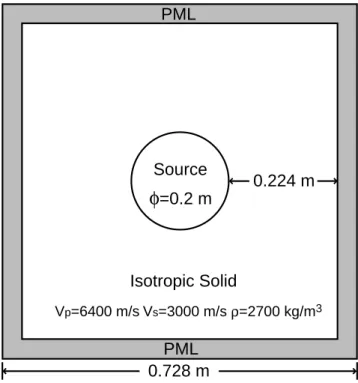
Figure 3 shows the layout of the computational domain and the absorbing boundary in Cartesian coor-dinates. PMLs are 10 grid thick and placed 0.224 meters away from the surface of the source, and the back boundary behind them is a stress-free space. Figure 4 illustrates the numerical result of the amplitude of the cylindrical wave in the 2D computational domain. The dark gray indicates high amplitude. The out-going wave appears strongest near the source and decays evenly along all radial directions. Its normalized amplitude along the x direction is plotted in Figure 5. As a cylindrical wave, its amplitude is proportional to pa/r, which is also plotted in the figure. The comparison of the amplitude results shows PMLs work effectively in a 2D FEM.

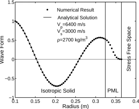
In order to solve the same problem in cylindrical coordinates, we now construct the PML as an infinite long ring centered along a z axis with the inner radius of 0.324 m and the thickness of 0.04 m. Again, the back boundary behind the PML is a stress free space. The dot plot in Figure 6 is the real part of the numerical solution, which represents a snapshot of the waveform at a certain time when the vibration of the source reaches the maximum amplitude. It is the same as the real part of a normalized Hankel function, Re[H0(2)(kpr)/H0(2)(kpa)], which is shown as the solid line in Figure 6. The agreement between these two results demonstrates the efficacy of the PML in cylindrical coordinates.

4.1.3 Spherical compressional wave

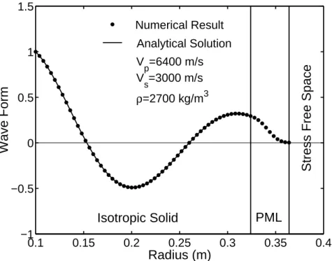
Suppose that a spherical source, whose radius is 0.1 m, is located at the coordinate origin performing a radial vibration. It is convenient to use the PML in spherical coordinates to solve this problem numerically. The PML is a 0.04 m thick spherical shell with an inner radius of 0.324 m surrounding the source. Behind the PML is a stress free boundary. The effectiveness of the PML is demonstrated in Figure 7 by the waveform from the numerical calculation along with the analytical solution, which is the real part of a normalized spherical Hankel function of the second kind, Re[h(2)0 (kpr)/h(2)0 (kpa)]. The amplitude of the outgoing spherical wave is proportional to a/r, as shown in Figure 8. Again, we get excellent agreement.

4.2

PMLs in the FDTD method

Beside their easy implementation in the FEM, our anisotropic PMLs for elastic waves can be applied to the FDTD method as well with no difficulty. In the FDTD, the particle velocity vector v is preferred over the displacement u in Eqs. (34) and (35). Therefore, the PML formula in Cartesian coordinates is

iωεxεyεzρv = ∇ · T, (84)

iωT = ˜C: ∇v. (85)

We note that in order to formulate a stable FDTD scheme and to implement the PMLs efficently, it is more convenient to use an interim strain-rate tensor than directly implementing the PML (Eqs. (84) and (85)) within FDTD. The interim strain-rate tensor E is defined as

Source

Isotropic Solid

PML

PML

0.224 m

φ

=0.2 m

0.728 m

Figure 3: Layout of the computational domain with a cylindrical monopole source located at the center. The PML is 10 grid wide at every boundary.

0.5

0.6

0.7

0.8

0.9

−0.3

−0.2

−0.1

0

0.1

0.2

0.3

−0.3

−0.2

−0.1

0

0.1

0.2

0.3

X (m)

Y (m)

Figure 4: Normalized amplitude distribution of a cylindrical compressional wave propagating in the compu-tational domain illustrated in Figure 3. The 2D FEM uses Cartesian coordinates. The dark gray indicates the high amplitude. The wave decays axisymmetrically along all radial directions.

0.1

0.15

0.2

0.25

0.3

0.35

0.4

0

0.2

0.4

0.6

0.8

1

1.2

X (m)

Normalized Wave Amplitude

Stress Free Space

Isotropic Solid

PML

Analytical Solution

Numerical Result

V

=6400 m/s V

=3000 m/s

ρ

=2700 kg/m

Figure 5: Comparison of the normalized amplitudes of the cylindrical compressional wave along the x di-rection computed with the analytical approach and those computed using the 2D FEM from Figure 4 in Cartesian coordinates.

0.1

0.15

0.2

0.25

0.3

0.35

0.4

−1

−0.5

0

0.5

1

1.5

Radius (m)

Wave Form

Stress Free Space

Isotropic Solid

PML

Analytical Solution

Numerical Result

V

=6400 m/s

V

=3000 m/s

ρ

=2700 kg/m

Figure 6: Comparison of the snapshots of the cylindrical compressional wave computed with the analytical approach and the FEM in cylindrical coordinates.

0.1

0.15

0.2

0.25

0.3

0.35

0.4

−1

−0.5

0

0.5

1

1.5

Radius (m)

Wave Form

Stress Free Space

Isotropic Solid

PML

Analytical Solution

Numerical Result

V

=6400 m/s

V

=3000 m/s

ρ

=2700 kg/m

Figure 7: Comparison of the snapshots of the spherical P wave computed with the analytical approach and the FEM in spherical coordinates.

0.1

0.15

0.2

0.25

0.3

0.35

0.4

0

0.2

0.4

0.6

0.8

1

1.2

Radius (m)

Normalized Wave Amplitude

Stress Free Space

Isotropic Solid

PML

Analytical Solution

Numerical Result

V

=6400 m/s

V

=3000 m/s

ρ

=2700 kg/m

Figure 8: Comparison of the normalized amplitudes of the spherical compressional wave computed with the analytical approach and the FEM in spherical coordinates.

Thus, the PML formulation becomes iωεxεyεzρv = ∇ · T, (87) iω εxεyεz Λ−1· T = C : E, (88) Λ−1· E = ∇v, (89) where Λ−1=       εx 0 0 0 εy 0 0 0 εz       , (90) Defining that εi= βi− iωαi, (91) A − iB/ω = εxεyεz, (92) and Ri− iΩi/ω = ½ ₁ εxεyεz Λ−1 ¾ ii , (93)

which only has diaganol entries, we then transform Eqs. (87), (88) and (89) into the time domain, and write them explicitly as ρ(A∂ ∂t + B)vi= {∇ · T}i, (94) (Ri ∂ ∂t+ Ωi)Tij = {C : E}ij, (95) (βi− αi ∂ ∂t)Eij = {∇v}ij. (96)

The subscripts i and j denote the entries in vectors and tensors.

Eqs. (94), (95) and (96) are the primary equations of the anisotropic PML for the FDTD method. When it is used in cylindrical and spherical coordinate systems, subscripts x, y and z should be replaced by the corresponding coordinates. This formulation of the PML is good for any isotropic or anisotropic solid medium. It is fully compatible with the FDTD method using staggered grids, and other advanced computational algorithms developed for the FDTD method. For more detail see Huang et al. (2002) in this report.

5

Conclusions

The new anisotropic PML formulation for elastic waves developed in this paper does not require the tedious work of field splitting, which is especially difficult when the medium is anisotropic and wave equations are complicated. It uses fewer unknowns and equations than the PML scheme with field splitting. Thus, computation with this PML is more efficient. To generate this numerical absorptive material, the stress tensor and the elasticity tensor must be considered asymmetric to allow the acoustic impedance of the absorptive medium matching that of the computational domain. The PML can be treated as a solid with anisotropic and complex elasticity properties, and a complex density. Although it is artificially created, wave propagation in this PML is governed by the same equation of motion and Hooke’s law as in the real solid material. For all three coordinate systems, the anisotropic PML can be expressed in one universal formula. Moreover, it is easy to implement the anisotropic PML not only in the FEM, but also in the FDTD method. The numerical results using the FEM confirm that this anisotropic PML has an extraordinary performance in absorbing outgoing waves within a short distance and results in negligible reflection. Its broad applications are promising in seismic and elastic wave simulation and modeling.

6

Acknowledgments

Y. Zheng would like to thank Prof. Robert E. Apfel in Physical Acoustics Lab at Yale University for the support of his research. This work was supported by the M.I.T. Borehole Acoustics and Logging Consor-tium, and by the Founding Members of the Earth Resources Laboratory at the Massachusetts Institute of Technology. It was also partially supported by NASA Grant #NAG3-2147.

References

Auld, B. A. (1973). Acoustic Fields and Waves in Solids. John Wiley & Sons, New York.

Berenger, J. P. (1994). A perfectly matched layer for the absorption of electromagnetic-waves. J. Comput. Phys., 114(2):185–200.

Chew, W. C. and Liu, Q. H. (1996). Perfectly matched layers for elastodynamics: A new absorbing boundary condition. J. Comput. Acoust., 4(4):341–359.

Chew, W. C. and Weedon, W. H. (1994). A 3d perfectly matched medium from modified maxwells equations with stretched coordinates. Microw. Opt. Technol. Lett., 7(13):599–604.

Hastings, F. D., Schneider, J. B., and Broschat, S. L. (1996). Application of the perfectly matched layer (pml) absorbing boundary condition to elastic wave propagation. J. Acoust. Soc. Am., 100(5):3061–3069. Huang, X., Zheng, Y., Burns, D. R., and Toks¨os, M. N. (2002). A stretching grid finite difference time-domain scheme implemented with anisotropic perfectly matched layer. In Earth Resources Laboratory 2002 Industry Consortium Meeting.

Kuzuoglu, M. and Mittra, R. (1997). Investigation of nonplanar perfectly matched absorbers for finite-element mesh truncation. IEEE Trans. Antennas Propag., 45(3):474–486.

Liu, Q. H. (1999). Perfectly matched layers for elastic waves in cylindrical and spherical coordinates. J. Acoust. Soc. Am., 105(4):2075–2084.

Maloney, J., Kesler, M., and Smith, G. (1997). Generalization of pml to cylindrical geometries. In Proc. 13th Annu. Rev. of Prog. Appl. Comp. Electromag., volume 2, pages 900–908, Monterey, CA.

Sacks, Z. S., Kingsland, D. M., Lee, R., and Lee, J. F. (1995). A perfectly matched anisotropic absorber for use as an absorbing boundary condition. IEEE Trans. Antennas Propag., 43(12):1460–1463.

Shlager, K. L. and Schneider, J. B. (1998). A survey of the finite-difference time-domain literature. In Taflove, A., editor, Adnvaces in Computational Electrodynamics: The Finite-Difference Time-Domain Method, chapter 1, pages 1–62. Artech House, Boston, MA.

Teixeira, F. L. and Chew, W. C. (1997a). Pml-fdtd in cylindrical and spherical grids. IEEE Microw. Guided Wave Lett., 7(9):285–287.

Teixeira, F. L. and Chew, W. C. (1997b). Systematic derivation of anisotropic pml absorbing media in cylindrical and spherical coordinates. IEEE Microw. Guided Wave Lett., 7(11):371–373.