Analysis of a forecasting-production-inventory system with stationary demand

UI

Massachusetts Institute of Technology

Sloan School of Management

Analysis of a Forecasting-Production-Inventory

System with Stationary Demand

L. Beril Toktay Lawrence M. Wein

April 1999

Working Paper Number 4070

Contact Address:

Prof. Lawrence M.Wein Sloan School of Management

Massachusetts Institute of Technology Cambridge, MA 02142-1343

Lwein@mit.edu

Analysis of a Forecasting-Production-Inventory

System with Stationary Demand

L. Beril Toktay INSEAD

77305 Fontainebleau, France and

Lawrence M. Wein

Sloan School of Management, MIT Cambridge, MA 02142

Abstract

We consider a production stage that produces a single item in a make-to-stock manner. Demand for finished goods is stationary. In each time period, an updated vector of demand forecasts over the forecast horizon becomes available for use in production decisions. We model the sequence of forecast update vectors using the Martingale Model of Forecast Evolution developed by Graves et al. (1986, 1998) and Heath and Jackson (1994). The production stage is modeled as a single-server discrete-time continuous-state queue. We focus on the stationary version of a class of policies that is shown to be optimal in the finite time horizon, deterministic-capacity case, and use an approximate analysis rooted in heavy traffic theory and random walk theory to obtain a closed-form expression for the (forecast-corrected) base-stock level that minimizes the expected steady-state inventory holding and backorder costs. This:expression, which is shown to be accurate under certain conditions in a simula-tion study, sheds some light on the interrelasimula-tionships among safety stock, stochastic correlated demand, inaccurate forecasts, and random and capacitated production in forecasting-production-inventory systems.

1. Introduction

In make-to-stock environments, manufacturers produce goods according to a forecast of future demands. Typically, within the confines of a materials requirement planning (MRP) system, future demands over a specific horizon are forecasted, these forecasts are revised each period in a rolling-horizon fashion, and production plans are updated accordingly. To better understand such forecasting-production-inventory settings, we analyze a discrete-time single-item make-to-stock queue facing a stationary demand process and rolling-horizon forecast updates. In our model, we envision forecasting and production-inventory control as decentralized activities: Forecasts are generated by a forecaster using some process (e.g., time-series methods, advance order informa-tion, expert judgement) that is unknown to the production manager. The production manager only observes a stream of forecast updates, and must convert these up-dates into a production policy that minimizes the expected steady-state holding and backorder costs of finished goods inventory. To perform this conversion in an effective manner, the production manager needs to have a characterization of both the demand and forecasting processes.

Graves et al. (1986, 1998) and Heath and Jackson (1994) have made great strides in enabling this characterization by independently developing a model for how fore-casts evolve in time, which is dubbed the Martingale Model of Forecast Evolution (MMFE) by Heath and Jackson. We employ this simple but deceptively powerful tool to model the inputs to our make-to-stock queue. Readers are referred to Heath and Jackson for an excellent literature review, where the MMFE is placed in the context of earlier attempts at modeling forecast evolution and alternative model-ing approaches (Bayesian, time-series, power approximations) to managmodel-ing inventory systems with uncertain demand.

The first MMFE paper was by Graves et al. (1986), who constructed a single-item version of the MMFE with independent and identically distributed (iid) demand and applied it in a two-stage setting, focusing on production smoothing and the disaggre-gation of an aggregate production plan across multiple items. Graves et al. (1998)

Ill

embedded the single-item MMFE with serial demand correlation within the linear systems model of Graves (1986), which corresponds to an uncapacitated system with deterministic lead times. For the case of a single-stage model and iid demand, they analytically optimized the tradeoff between production smoothing (i.e., standard de-viation of production) and safety stock (i.e., standard dede-viation of inventory). They also showed how to use the single-stage model as a building block for a multistage acyclic system. Unaware of Graves et al. (1986), Heath and Jackson developed an MMFE for a multiproduct system that accounts for correlations in demands across products and across time periods. They used the MMFE to generate forecast up-dates in their simulation of an existing LP-based production-distribution system and demonstrated how improved forecasts could reduce safety stocks without affecting service performance. Using a special case of the MMFE, Giillii (1996) considered a single-item system with instantaneous but capacitated production and uncorrelated demand, and showed that the system performs better when a demand forecast for one period into the future is employed. Chen et al. (1999) illustrated their stochastic dy-namic programming algorithm based on experimental design and regression splines by numerically computing the optimal ordering quantities for an inventory system with instantaneous replenishment that is driven by the MMFE.

A related paper that does not employ the MMFE is Buzacott and Shanthiku-mar (1994), who analyzed the safety stock versus safety time tradeoff in a capacitated continuous-time MRP system with iid demands that are known exactly over a fixed time horizon. Karaesmen et al. (1999) developed a dynamic programming formula-tion of a discretized, Markovian version of the Buzacott-Shanthikumar model with unit demand and productions in each period, and showed computationally that the value of advance information decreases with system utilization. There is also a stream of literature that ignores the capacitated nature of the production environment and uses alternative models to incorporate forecasts of stationary demand in inventory management decisions (e.g., Veinott 1965, Johnson and Thompson 1975, Miller 1986, Badinelli 1990, Lovejoy 1992, Drezner et al. 1996, Chen et al. 1997, Aviv 1998). To our knowledge, this paper contains the first analysis of a capacitated

production-inventory model facing a general stationary stochastic demand process and dynamic forecast updates.

The remainder of the paper is organized as follows. The MMFE is described in §2.1 and the production-inventory model is presented in §2.2. Dynamic programming is used in §2.2 to show that the optimal policy in the finite time horizon, deterministic-capacity case is a modified (by deterministic-capacity restrictions) base-stock policy with respect to the forecast-corrected inventory level, which is the inventory level minus the to-tal expected demand over the forecast horizon; we consider a stationary version of this policy in §3. Heavy traffic analysis and tail asymptotics for random walks are combined in a heuristic manner in §3.1 to obtain a closed-form expression for the forecast-corrected base-stock level that minimizes the expected steady-state inven-tory holding and backorder costs. In §3.2, we numerically assess the accuracy of the derived base-stock level in some special cases. The managerial implications of this analysis are provided in §4, where we interpret the results in §3.1 and use them to address the following questions: How does forecast information impact base-stock lev-els? How can forecast quality in the context of production-inventory management be characterized? What is the relative value of correctly specifying a time-series forecast model versus optimally using the available forecast information? Possible extensions

of the model are briefly discussed in §5.

2. The Model

The single-item version of the MMFE is described in §2.1. In §2.2, we formulate the production control problem of minimizing expected steady-state inventory holding and backorder costs in a single-stage production-inventory system that is driven by forecast updates, and motivate our use of a modified forecast-corrected base-stock policy.

2.1. The Martingale Model of Forecast Evolution

In each period, as additional information becomes available, the forecaster generates a new demand forecast for a single item for all periods in the forecast horizon. The difference between this vector of demand forecasts and the one that was generated in

III

the previous period is called the forecast update vector. The MMFE is a descriptive model that characterizes the resulting sequence of forecast update vectors.

Let Dt denote the actual demand in period t. The demand process {Dt} is assumed to be stationary with E[Dt] = A. Let Dt,t+i be the forecast made in period t for demand in period t + i, i = 0, 1,...; we assume that forecasts are made after current demand information is revealed, so that Dt,t = Dt. Let H be the forecast horizon over which nontrivial forecasts are available: We assume Dt,t+i = A and Cov(Dt, Dt+i) = 0 for i > H. Then et,t+i = Dt,t+i - Dt-l,t+i is the forecast update for period t + i

demand recorded at the beginning of period t (with t,t+i = 0 for i > H), and

Et = (t,t, Et,t+l,... , t,t+H) is the forecast update vector recorded at the beginning of period t.

Heath and Jackson essentially assume that the forecast represents the conditional expectation of demand given all available information, which implies forecasts are unbiased and forecast updates are uncorrelated (for brevity's sake, we refer readers to pages 21-22 of Heath and Jackson for details). Under these relatively mild assump-tions, the MMFE posits that {Et} forms an iid N(O, E) sequence of random vectors. To use the MMFE in modeling the observed forecast update process, the production manager only has to estimate the components of the (H + 1) x (H + 1) covariance matrix E from historical forecast updates (see page 23 of Heath and Jackson for a discussion of parameter estimation); for convenience, we index the elements of by

oij, i,j = O,... ,H. Note that the MMFE is a model of an existing forecasting process, and not a forecasting tool.

The following proposition demonstrates the correspondence between the parame-ters of the MMFE and the autocovariance structure of demand. All propositions are proved in the Appendix.

Proposition 1 If the MMFE assumptions are satisfied, then the true autocovariance

structure of demand can be recovered from the covariance matrix E via

H-i

7Yi Cov(Dt, Dt+i)

=

ajj+i for i = 0,1, ... ,H. (1)

Graves et al. (1986) assumed that the covariance matrix E was diagonal, which H

is equivalent to assuming that demand is iid with Var(Dt) = jj. Graves et j=o

al. (1998) and Heath and Jackson allowed a general covariance matrix, which arises when demand exhibits correlation. Note that this structure can capture correlations among forecast updates for future periods that are made in a given period. As noted by Heath and Jackson, the MMFE is preferable to a direct time-series approach (Box and Jenkins, 1970) in the production-inventory setting because it can model forecast updates arising from both an autoregressive moving average (ARMA) forecast model and from a variety of realistic informational structures (e.g., forecasts are generated by expert judgment, demand is known a fixed number of periods in advance, or total demand for the next quarter is known with more certainty than the breakdown by month).

The assumptions of the MMFE may fail to hold in practice. For example, if the forecaster is using an ARMA(p, q) model to forecast stationary demand, but does not specify its parameters correctly, the resulting sequence et} of forecast update vectors will be correlated, thereby violating the MMFE assumptions. Notice that "satisfying the MMFE assumptions" is a more general concept than "correctly specifying an ARMA model" because the MMFE does not limit the forecaster to the use of time-series models only. In this section and the next, we assume that the assumptions of the MMFE are satisfied; at the end of §4, we investigate the impact of equation (1) failing to hold due to the misspecification of a time-series model by the forecaster.

2.2. The Production-Inventory Model

Our production-inventory model is a single-server discrete-time continuous-state make-to-stock queue that is driven by a forecast update process modeled by the MMFE introduced in §2.1. Let Ct be the production capacity (i.e., maximum number of service completions) in period t. We assume that the sequence Ct} is iid N(u, oU), with _{> A to ensure stability. Define It to be the inventory level at the end of} period t. At the beginning of period t, the current demand is observed and the fore-casts are updated. Based on this information, the production quantity Pt E [0, Ct] is determined. Demands are satisfied using on-hand inventory and the newly

man-III

ufactured units. Hence, the end-of-period inventory level evolves according to the relation It = It_- + Pt - Dt. The one-period cost is h+ + bI-, where h and b are the unit inventory holding and backorder costs, respectively. Our goal is to find a production policy {Pt} to minimize the total expected steady-state inventory holding and backorder costs, hE[I+] + bE[I].

To motivate the form of the production policy analyzed in §3, we briefly consider the dynamic programming formulation of the finite time horizon problem with deter-ministic capacity. It is convenient to define a new state variable It = It - H=1Dt,t+i, which we call the forecast-corrected inventory level; it is the current inventory level mi-nus the total forecasted demand over the forecast horizon. This gives It = It-1 + Pt

-(A + eT Et), which is a state evolution equation with iid random variables (throughout the paper, e is a column vector of ones). This transformation allows us to prove the following result using methods from Federgruen and Zipkin (1986b), who analyzed the production-inventory problem with iid demand.

Proposition 2 For the finite-time horizon problem with deterministic capacity, the

optimal production policy is characterized by a sequence of scalars {B1, .. ., BT} and has the form

Ct ~ if Bt > It-l + Ct;

Pt(It_1) = Bt- It-1 if It_ < Bt < It-_ + Ct; (2)

0 if Bt < t-l.

The quantity Bt in (2) is an order-up-to, or base-stock, level with respect to the forecast-corrected inventory level, It-, and the optimal production policy is a modified base-stock policy, where the modification is due to the capacity constraint

Pt < Ct.

In the long-run average cost case with discrete iid demand and deterministic ca-pacity, Federgruen and Zipkin (1986a) show that a stationary modified base-stock policy is optimal. Federgruen and Zipkin (1986b) show that this policy is optimal in the infinite-horizon, discounted-cost case with continuous iid demand. We have

not attempted to generalize Proposition 2 to these cases. However, Proposition 2, Federgruen and Zipkin's results, and the attractiveness (with respect to analytical tractability and ease of implementation) of a stationary base-stock policy lead us to consider a stationary version of the modified forecast-corrected base-stock policy for the steady-state, random-capacity problem.

As is typical for make-to-stock queues (e.g., Chapter 4 of Buzacott and Shanthiku-mar 1993), we define this production policy in terms of a release policy. Let Rt denote the number of order releases to the production stage at the beginning of period t and Qt be the number of items at the production stage at the end of period t, called the work-in-process (WIP) inventory. The production quantity is characterized by the release policy via Pt = min(Qt_l + Rt, Ct).

As we show below, a modified base-stock policy with respect to the forecast-corrected inventory process It is constructed by setting Rt equal to the aggregate forecast update over the forecast horizon plus the new demand forecast for the last period of the horizon (see Buzacott and Shanthikumar 1994 for a similar policy). Using the above notation,

H-1 H

Rt = e Et,t+i + Dt,t+H = A + et,t+i = A + eTEt.

i=O i=O

Note that Rt} is an iid sequence and a dip in projected demand can cause negative releases, but these negative releases are not of grave concern because the release policy is simply a convenient way to define the production policy.

Suppose Qo = 0 and Io = SH + =lEH Doi, so that we initially stock enough items to satisfy the forecasted demand over the forecast horizon H plus a safety stock, H. Then

H

Qt,+It-

Dt,t+i =Qt + It=SH for t=1,2, ....

i=l

We call SH the forecast-corrected base stock level. Under this policy and the above

initial conditions, our production control problem is to find the forecast-corrected base-stock level s that minimizes hE[I+(sH)] + bE[Io(sH)], where we have intro-duced the dependence of the steady-state inventory level on the forecast-corrected base-stock level.

III

As a benchmark in our subsequent analysis, we also consider a myopic policy, where forecasts satisfying the MMFE assumption are available, but are not exploited in determining releases; that is, the production manager sets Rt = Dt. Note that the

autocovariance structure of {Rt} can be determined using equation (1). Under this myopic policy, and initial conditions Qo = 0 and 10 = Sm, the relation Qt + It = Sm

holds in every period. Let s denote the corresponding optimal base-stock level within this class of policies.

3. Main Results

In §3.1, we heuristically combine results from random walks and heavy traffic ap-proximations of queues to determine closed-form expressions for s and s in heavy traffic. The accuracy of our approximate analysis is investigated using simulation in

§3.2.

3.1. Analytical Results

We start by analyzing the steady-state WIP distribution using heavy traffic theory, which is an asymptotic method based on the system utilization p A A/L approaching

one.

Proposition 3 In heavy traffic, Qoo has an exponential distribution with parameter

2(p- A) 2(p- A)

T~e+ u 2Z c

e e + (TC t + 2 i=1 iYi + 'C

under both the forecast-corrected base-stock policy and the myopic policy.

A complementary asymptotic approach to discrete-time make-to-stock queues has been developed by Glasserman and co-workers. More specifically, Glasserman and Liu (1997) use Siegmund's (1979) method for a corrected diffusion approximation of random walks to analyze a discrete-time make-to-stock queue with iid demand. They

show that P(QOO > x) = e- _(x+P3)_+o( 2_{) as A - , x - o and (A-p)x -+ constant,}

where = 2(;--) (which is consistent with v in Proposition 3 in the iid demand case) and the correction term (specialized to the case where demand is iid normal with

variance a2 ) is P = 0.583 2a + C. Comparing Proposition 3 with Glasserman and

Liu's result allows us to see the relative strengths of both approaches: Heavy traffic analysis yields the entire distribution rather than just the right tail, and appears to more easily incorporate non-iid demand, whereas the random walk approximation is more accurate because it incorporates a higher-order correction term.

Hereafter, we employ the following approximation to the steady-state WIP distri-bution:

P(QO = ) = 1-e- _v3 _{and P(Q > x) =e}- _(xZ+3_{) for x > 0. (3)}

Equation (3) combines the relative strengths of both approaches in a heuristic manner. From Proposition 3, it uses the shape of the distribution (except for a pulse at the origin) and the heavy traffic term eTEe, even for the myopic policy where releases are correlated. Equation (3) also uses the corrected diffusion term from Glasserman and Liu. Simulation results in Toktay (1998) show that (3) is indeed more accurate than the heavy traffic approximation in Proposition 3 in the iid demand case.

Our main analytical results are collected in Proposition 4. Because the character-ization of the base stock level in Proposition 4b is difficult to work with, we consider the asymptotic case where b >> h in Proposition 4c (the "a" in sa is mnemonic for

"asymptotic").

Proposition 4 Using approximation (3),

a. The optimal base-stock level under the myopic policy is s = F h) = n(1 + ) -/. The optimal cost is Cm = hs* + h(-e-)

b. The optimal base-stock level under the forecast-corrected base stock policy with forecast horizon H is = Fi 1(b), where W = max{Q + Y, maxl<k<H Yk} and

H H k H+i H

Yk = -kA +

Z Z

6

t-H+i,t-H+j -

Z

Et-H+i,t-H+j-

Z

Ct-H+i-i=k+l j=i i=1 j=H+l i=k+l

c. For b >> h, SH is well approximated by s = Sm + /lyo + oio', and the optimal

cost CH = hE[I+ (s*)] +bEfI (s*)] is well approximated by CH = h(s + -E[W]), where ,yo and 2O are the mean and variance of Yo.

Proposition 4c is the central result of the paper. However, to obtain this reasonably tractable form for the forecast-corrected base-stock level, we made a series of approxi-mations: The heavy traffic approximation in Proposition 3, the heuristic combination of heavy traffic and random walk asymptotics in (3), and Clark's (1961) approxima-tion and several b >> h approximaapproxima-tions in estimating Fw(w) in the proof of Propo-sition 4c. Hence, we expect the accuracy of sa in PropoPropo-sition 4c to improve as the cost ratio b/h and the system utilization p increase, and - to a lesser extent - as the forecast horizon H decreases (see the comment under (11)).

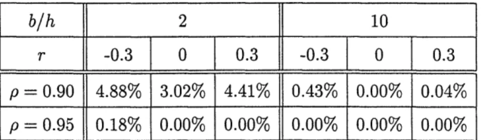
To assess the accuracy of s, we use discrete-event simulation to estimate the steady-state cost incurred by the forecasting-production-inventory system when it is operating under a forecast-corrected base-stock policy. Let s* denote the optimal base-stock level determined by an exhaustive search via simulation, and let C(s) be the simulated cost of the forecast-corrected base-stock policy with base-stock level s. All scenarios in this paper were simulated until the 95% confidence interval width fell below 1.0% of the average cost.

b/h 2 10

r

-0.3

0 0.3

-0.3

0 1 0.3

p = 0.90 4.88% 3.02% 4.41% 0.43% 0.00% 0.04%

p= 0.95 0.18% 0.00% 0.00% 0.00%0.00% 0.00%

Table 1: The simulated cost suboptimality of the derived base-stock level, st, for MA(1) demands. Parameter values: ar = cc = 10, / = 100, h = 1.

For concreteness, we assume that demand follows a moving average process of lag 1, which is abbreviated by MA(1). Thus, Dt = A + et - Olet-1, where the et's are iid N(0, a2). The forecast horizon is H = 1, and forecasts are given by Dt,t+l = A - Olet, Dt,t+i = A, i > 1, giving rise to forecast update vectors of the

form et = (1,-01)et. Table 1 compares the cost suboptimality, C (s*), for various values of the backorder-to-holding cost ratio b/h, the system utilization p and the demand correlation r = -01. This table reveals that sa is very accurate when p =

0.95, and the cost suboptimality is below 5.0% even when p = 0.9 and b/h = 2. To investigate the robustness with respect to the forecast horizon H, we also simulated a case with a MA(5) demand process (where H = 5) with i = -0.3 for i = 1, 2,..., 5, and b/h = 10; the cost suboptimality was 5.62% when p = 0.9 and 0.00% when

p = 0.95. Hence the derived base-stock level appears to be reasonably robust with

respect to the forecast horizon H.

4. Discussion

In this section we record some observations about Proposition 4.

iid demand, no advance demand information. In the traditional case where

demand is iid with variance a2 and no advance demand information is available, the forecast horizon H = 0, Yo = 0 and W = Qc. The optimal base stock level in Propo-sition 4b is s = -l ln(1 +

))-/,

where v reduces to .2(~-x The optimal base-stock level increases with system utilization, the variability of service capacity and the vari-ability of demand. This result coincides with Glasserman's (1997) asymptotic result, which uses approximations to tail probabilities for random walks (e.g., Siegmund

1985) but does not use Glasserman and Liu's corrected diffusion approximation.

Correlated demands, myopic policy. If demands are correlated, but the myopic

production policy is used, then equation (3) and Proposition 4a imply that posi-tively (negaposi-tively, respecposi-tively) correlated demands increase (decrease, respecposi-tively) the basestock level and according to a secondorder Taylor series approximation -the resulting cost.

Interpretation of Y. When b >> h, the forecast-corrected base-stock level in Proposition 4c is expressed as the myopic base stock level s plus several terms that incorporate the random variable YO. To interpret YO, let us define Ft,t+i = Dt+i-Dt,t+i, which is the error in the forecast made at time t in estimating time t + i demand. It

H H

can be shown that Yo = Ft-H,t-H+i-E Ct-H+i. The stationarity of the underlying

i=l i=l

demand and production processes implies that Y is independent of t, and thus it can be interpreted as the error in the forecast of total demand over any forecast horizon of H periods minus the total production capacity over this forecast horizon.

Ill

By construction, Dt,t+i, i = 1, 2, ... , H} and Ft,t+i, i = 1, 2,... , H} are given

in terms of {Et-H+i, i - 1,2,... ,H} and {Et+i, i = 1,2,... ,H}, respectively. Thus, H=_{1 Dt,t+i and} EH Ft,t+i are independent. The total demand over a fore-cast horizon of H periods can be written as i Dt== H=1 1 ,t+i + .= Ftt+i

By independence, Var( 1 Dt+i) = Var i=1 Dt,t+i) + Var i Ft,t+i) Thus,

Var(ZiH Ft,t+i) represents the total demand variability over an H-period forecast

horizon that has not been resolved as of the beginning of that horizon. The total system (demand and production) variability over this horizon is Var(ZH 1 Dt+i) + Var(H 1 Ct+i), so Var(Yo) is the portion of total system variability over an H-period

forecast horizon that is as yet unresolved at the beginning of that horizon.

Forecast quality. The interpretation of Yo suggests the following definition of forecast quality from the production manager's viewpoint.

Definition 1 Let EA and EB correspond to two different forecasting schemes for the same demand process that both satisfy the MMFE assumptions. Then forecasting scheme A is better than forecasting scheme B if

H H

Var( Ftt+i) < Var(Z Ft,+i) Vt (4)

i=l i=1

Condition (4) states that forecast quality is characterized by the unresolved demand variability over the forecast horizon. We can express this quantity in terms of the

H

covariance matrix by Var(E Ft,t+i) =

zN

1 fTEfi, where

fi

is a

column vector with

i=l

i ones followed by H + 1 - i zeroes.

Proposition 5 If forecasting scheme A is better than forecasting scheme B according

to (), then ()A _<(s)B and (C)A <(C)B.

Thus, systems using a better forecast (even within the restriction of the forecast already being "good" in the sense that it is unbiased and correctly captures the covariance matrix) will hold less safety stock. A better forecast also leads to a lower cost when H = 1 (i.e., the demand autocovariance function has one lag ); the H > 1 case remains open.

Interpretation of Proposition 4c: The iid demand case. Suppose demand is

iid with variance U but advance demand information may be available. The set of covariance matrices corresponding to all possible forecast structures consistent with iid demand is given by Eiid = ({ IE = diag( H=o 2,2, ,r 2H), 2 = cHD}.

In

this setting, Dt = A + ZEH=OEt-i,t where the forecast updates et-i,t are independent

and N(O, o2) for i = O,..., H, and Et-i,t represents the number of units ordered (or

cancelled) i periods in advance for delivery in period t. Here, Var(H 1Dt,t+i ) = X1 ici, Var(E i F+i) =l t = (H - i)ua and Var(E i 1 Dt+i) = HU.

Let us consider the two extreme cases: If the forecaster has no advance infor-mation about demands then E = diag(a,

o,...

,0), Var(E ₁Ft,t+i) = Ha2 and Var(ZEH 1 Dt,t+i) = 0. Although this situation corresponds to a natural forecast

hori-zon of zero, this general framework allows us to make a consistent (i.e., common forecast horizon) comparison of the forecast-corrected base stock levels under fore-casting processes with E Eiid. At the other extreme, if the forecaster receives exact information about demand H periods ahead then E = diag(O, 0,... ,2H),

Var(H 1 Ft,t+i) = 0 and Var(:iH 1 Dt,t+i) = Ha2.

By Proposition 4c, sH = sm + o + yV = * - Hp + [Var(E 1 Ft,t+i) +

Var(Zi= 1

Ct+i)]

eTJ.e+) ' If demand is iid then sm = so, eTEe = U2 and

level, _{Equation (5) reduces to st revealin} SH=H-S-Hp. _{- H andresult. It shows - H - H(reduction in the} base-respectively, in the two extreme case of no advance information s and full advance

information. In all casesH , which 0 < iaH the 1; right inequality is tight in the full information case with deterministic capacity, which leads to the minimum base stock

level, s = s - Ht~.

Equation (5) is our most revealing result. It shows that the reduction in the base-stock level from the case of no advance information is the product of two factors: The first factor is H(/p-A), which is the total expected excess production capacity over the forecast horizon. The second factor in the reduction term is a fraction: The numerator is the demand variability over the forecast horizon that has been resolved already,

Ill

and the denominator is the total system (i.e., demand and production) variability over the forecast horizon. Thus the reduction is that fraction of expected excess production capacity over the forecast horizon that equals the proportion of the total variability over the forecast horizon that has already been resolved. This highlights the interchangeability of excess production capacity and safety stock as alternative resources in make-to-stock queues: The earlier the demand variability is resolved, the more the system can rely on excess production capacity (as opposed to safety stock) to counter demand variability.

Interpretation of Proposition 4c: The general case. For the non-iid demand

case, repeating the calculations leading to (5) yields

H

/

Var(Z Ft+i) + H c

= S-HA-H(u-A) - HeTe + H

)(6)

Here, s - HA does not represent an appropriate benchmark for comparison when demand is not iid, because it assumes -H Dt,t+i = HA (which violates the MMFE

assumption) and =EH Dt,t+i is independent of Qt (which ignores information about

demand correlation contained in previous demands). Moreover, Var(Hel Ftet+)o-HC is

not a proper fraction because eTEe is the variance of the limiting Brownian motion corresponding to the demand process, and hence HeTEe is a measure of - but does not equal - the total demand variance over the forecast horizon. Nonetheless, by (6), it still follows that the optimal base-stock level increases with the amount of unresolved system variability over the forecast horizon.

Heavy traffic limit. From equations (5) and (6), we see that s -+ s - HA as the

system utilization p -+ 1. Hence, the value of using forecast information vanishes as the traffic intensity approaches unity. In this case, there is very little excess capacity (i.e., H(u - A) is small) to satisfy unresolved forecasted demand, and safety stock

must be used instead. This observation is similar in spirit to an observation in §5.6 of Markowitz and Wein (1998), who show analytically that reducing due-date lead times in a make-to-stock system does not improve system performance in the heavy traffic limit. This observation is also consistent with the computational results in Karaesmen et al.

Forecast bias and temporal forecast aggregation. The MMFE assumes that the

sequence {(t) of forecast update vectors is id N(O, E). The remainder of this section explores the two natural violations of this assumption by an erroneous forecaster: The mean of Et is not zero (due to forecast bias) and the sequence {(Et is not iid (which can occur because the forecaster has not used all available information about past demands).

Proposition 4 implies that if the forecaster overestimates (underestimates, respec-tively) the average demand A, then the production manager using this forecast will carry too much (too little, respectively) safety stock, leading to suboptimal perfor-mance. Here we discuss a more subtle type of forecast bias, where the forecast update vector Et is such that E[eTEt] = 0 but E[Et,t+i] = mi # 0, i = 0, 1, ... , H. That is,

the mean demand A has been identified correctly but the forecast made at time t for demand at time t + i is biased (i.e., E[Dt,t+i] = A + =i m).

If the production manager recognizes the existence of the bias, then he can reduce the base-stock level sH in Proposition 4c (which is optimal for unbiased forecasts)

by the bias in the forecast of total demand over the forecast horizon H,

EH1

imi,

and performance will not suffer. If this bias is not recognized then the base stock level and the resulting cost will be suboptimal. However, in this case we suspect that temporal aggregation of the forecast might improve performance by decreasing the forecast bias; for example, if a forecaster has an unbiased estimate of the total demand over the next quarter, but biased estimates of the individual monthly demands, then performance might be improved by using a quarterly forecast in production decisions rather than a monthly forecast. However, a discrete-time model - where releases and demands occur with the same frequency and costs are assessed at the end of the period - is unable to accurately capture the cost tradeoff between improved forecast accuracy and the loss of information and increased system variability due to temporal aggregation.

Relative value of forecast model specification versus forecast use. In the

remainder of this section, we assume that the forecaster takes a time-series approach, the first step of which is forecast model specification. The effective management of

III

our forecasting-production-inventory system requires the correct specification of the forecast model by the forecaster and the appropriate use of the forecast information by the production manager. However, each of these steps may be performed incorrectly in practice, and we conclude this section by using discrete-event simulation to investigate this possibility. More specifically, we consider three different scenarios to compare the impact of misspecifying the forecast model versus the impact of failing to incorporate forecast information from a correctly specified model into the production decisions. In all three scenarios, we assume that demand has an autocovariance function of H lags. In the first scenario, the forecaster incorrectly thinks that demand is iid and no advance demand information is available. In this case, the forecaster's update vector Et contains only the element tt = Dt - A. The production manager sets the forecast horizon H = 0 and recovers only the unconditional demand variance. (Notice that, unbeknownst to the production manager, the sequence {et} is correlated and does not

satisfy the iid assumption of the MMFE.) By an adaptation of Proposition 4a to this case, we see that the production manager who receives this incorrect forecast employs a base stock policy with respect to the actual inventory level with the suboptimal base stock level Siid viid ln(1 +

)

- iid, where = 2iid + and iid = 0.583

To assess the cost ramifications of the forecaster's erroneous iid assumption, we consider a second scenario where a different forecaster correctly specifies the forecast model, but the production manager who receives this forecast fails to use it in an optimal manner, instead employing the myopic production policy defined at the end of §2, with the base stock level s specified in Proposition 4a. Note that here the production manager recovers the true autocovariance structure of demand and uses it in calculating s. A comparison of the first two scenarios allows us to isolate the cost of forecast model misspecification because both production managers are using the release policy Rt = Dt.

Finally, we consider a third scenario where the forecast-corrected base-stock policy is used, with base-stock level s from Proposition 4c. Comparison of the second and third scenarios allows us to evaluate the impact of using forecast information to determine the production policy: The autocovariance structure of the demand process

is correctly identified in both cases, but the myopic policy fails to use the forecast information in its production decisions.

0 1) 3 en 0.8 0.6 0.4 0.2 0 0.2 0.4 0.6 0.8 demand correlation

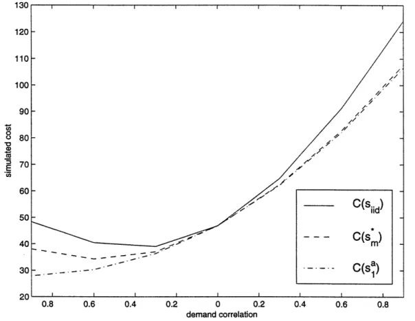
Figure 1: Comparison of simulated costs under three scenarios for MA(1) demands. In the top curve, the forecaster incorrectly believes that demand is iid; in the middle curve, the forecast model is correctly specified but the myopic policy is used; in the lower curve, the forecast model is correctly specified and the forecast-corrected base-stock policy is used. Parameters: a = ac = 10, A = 95, /l = 100, h = 1 and

b= 10.

The simulated costs C(siid), C(s*) and C(s') are plotted as a function of the demand correlation r in Figure 1 for a MA(1) demand process. Comparing the first two scenarios (the top two curves in Figure 1), we see that when the demand correlation r = 0, demand is iid and C(s,) = C(Siid). As expected, the difference between the cost curves increases as Irl -+ 1; in fact, using Proposition 4a we can show that the cost difference between the top two curves is locally convex in r at

r= O.

A comparison of the bottom two curves in Figure 1 shows that the forecast-corrected base-stock policy outperforms the myopic policy, as expected. For a fixed value of Irl, the cost deviation between the bottom two curves in Figure 1 is more severe when demand is negatively correlated. This can be explained by equation (6), which reduces in this case to s = Sm - + 2(1+r)f2+ (, - A). Simulation results in Toktay demonstrate more generally that the lowest cost is achieved when the production manager uses forecast information about demands over the entire forecast horizon, rather than just a portion of the horizon.

A comparison of all three curves in Figure 1 demonstrates that greater cost in-creases are incurred if the forecaster incorrectly specifies the forecast model than if the production manager fails to use forecasts from a correctly-specified model in his production decisions. We have been unable to assess analytically whether this claim holds in broad generality. However, a similar set of curves (not shown here) for a

MA(5) demand process gives the same qualitative results. Hence, our results suggest

that under reasonably high system utilization, the main value of forecasting stems from the specification stage, which arguably is not carried out thoroughly in practice. It would thus be of considerable value to design production-inventory policies that are robust to forecast model misspecification.

5. Extensions

Two natural extensions of this work are to multiple items and multiple stages. Heavy traffic theory for continuous-time multiclass queues is well developed and Heath and Jackson have developed a multi-item MMFE, suggesting that the multi-item extension should not be very difficult. However, care must be taken in defining - and analyzing in heavy traffic - a queueing discipline in discrete time. An interesting empirical and theoretical question in this context is the relative contribution to the safety stock of the demand correlation across time versus the demand correlation across products. Extending our analysis to a multistage model would be much more difficult, in light of the analytical intractability of Markovian tandem make-to-stock queueing systems

(e.g., Veatch and Wein 1994). One tractable approach (see Rubio and Wein 1996) is to employ a CONWIP policy that maintains the total forecast-corrected WIP plus finished goods inventory (i.e., Qs + It- =l Dt,t+i, where Q is the system-wide

WIP) at a constant base-stock level.

Appendix

H

Proof of Proposition 1: The MMFE assumptions imply that Dt = A +

Z

Et-H+j,t j=o

Therefore

i - Cov(Dt,Dt+j) = E[(Dt- A)(Dt+i- A)]

H H

= E[(> t-H+j,t) ( Et+i-H+j,t+i)]

j=O j=O

H-i

= E[et+i-H+j,tet+i-H+j,t+i] _{because forecast updates are uncorrelated} j=O

H-i H-i

-=

3

H-i-j,H-j = - aoj,j+i.

j=O j=O

Proof of Proposition 2: The dynamic programming algorithm for the finite time

horizon problem is

JT+1 (IT) = 0 (assuming no salvage value or disposal cost)

Jt(it-,) = min {Eet[h(It-l + Pt + i=1 t-lt +i

-O<Pt<Ct

+- •H-1

+b(it-l + Pt + Dt-lt+i - tt)-]

+Eet[Jt+l(it- + Pt - ( + eTet))]}, t E {1, 2, ... , T}.

Here, It_l+Pt+EZ-H= 1_Dt- l_,t+i - _{= = I+Pt-D= tt}

It and It_l+Pt-(A+eT _{et) = It.} If we define Yt = It- + Pt, wt = tt - fHl Dt-l,t+i, Ht(yt) = hEet[(yt - wt)+_{] +}

bEt[(yt - wt)-] and Gt(yt) = Ht(yt) + E[Jt+l(yt - (A + eTet)], then the dynamic programming algorithm can be expressed as

JT+1 (t) = 0

Jt(It-1) = min Gt(yt), t E {1,2,...,T}. It-1<Yt< i- l+Ct

III

It can be shown inductively as in Federgruen and Zipkin (1986b) that Gt(yt) is convex and limly,,l,, Gt(yt) = oo. This implies Gt(yt) has an unconstrained minimum with respect to Yt for all t. Let Bt = argminy, Gt(yt) and yt = arg minilyt<ht_l+ct Gt(yt). Then

it_ i+Ct if It_ < Bt - Ct;

Yt = Bt if Bt- Ct < t-_ < Bt;

It_~1 if it-_ > Bt, which yields (2).

The induction proof uses the facts that for all t, Ht(yt) is convex in Yt, limlytl-oO Ht(yt) =

c, Jt > 0, and if Bt minimizes Gt then

Gt(It_- + Ct) if It- < Bt - Ct; Jt(_-1) = Gt(Bt) if Bt- Ct < t_1 < Bt;

Gt (It-,) if It-1 > Bt is a convex function.

Proof of Proposition 3: Let Et = Rt- Ct and X. =

Lt=

1Et. Then Qn =

X,-infl<t< Xt. Take a sequence of systems indexed by k with A(k) -+ A and p(k) -_+ such that vk-( AX(k)()) -+ c < 0, where c = 0(1). Note that Qk) = X(k)-infl<t<n Xt(k) = Xk) - nm(k) + nm(k) + y(k) where m(k) = A(k) _ (k) and (k) = - infl<t< Xk). If

(k) X(k) y(k)

we define Qk(t) =

_,J

Xk(t) = tJ and Yk(t) = , then Ok(t) = Xk(t) + ?k(t)

__M _ m_ kttJ ____

X(k) _m(k)LktJ

W-mixing processes (Thm. 20.1 in Billingsley 1968), lkt J jB(t), a where

C2 = Var(Ro - Co) + 2 ]t°l Cov(Ro - Co, Rt - Ct) and B is standard Brownian

motion. Since the {Ct} are iid and independent of the releases, i 2 = Var(Ro) +

Var(Co) + 2 E'=1 Cov(Ro, Rt). Under the forecast-corrected base-stock policy,

re-leases are iid with Rt - N(A, eTEe) and U2 = eTEe + a2c. Under the myopic policy,

Rt = Dt and Var(Ro) + 2 °°l Cov(Ro, Rt) = Var(Do) + 2

Ef

1

l Cov(Do, Dt) =

-yo

+ 2 t'H= t = eTEe, where the last equality follows from equation (1).

Further-more, the assumption v( A(k) - L(k)) -+ c implies that m - ct. Therefore,

with drift 0 and variance eTEe + ac. If we define 0(x)(t) = - info<s<t{x(s)} and +(x)(t) = x + q(x)(t), where x is a right-continuous left-limit process with x(O) = 0, then (Qk(t), Yk(t)) = (4, q)(Xk(t)). Since we have established that Xk = X*, where X* is B(c, eTEe +

Ua),

a process with continuous sample paths, the continuous mapping theorem (Thm. 5.1 in Billingsley) implies that (, )(Xk) converges to (4, +)(X*), i.e, Qk =. Q*, where Q* is RBM(c, eTEe + c ) on [O,oo), which is a

reflected Brownian motion on the nonnegative halfline. The steady-state distribu-tion of RBM(c, a2) is exponential with parameter 2 (Harrison 1985). Reversing

the heavy traffic scaling, we estimate the steady-state WIP QOC by an exponential random variable with parameter vee2lc _21c - ₌ e _2(/h-A)(e+)

Proof of Proposition 4:

4a. Since It = sm - Qt for all t, we have Ioo = Sm - Qo Let C(sm) =

hE[I+(sm)] + bE[I~(sm)], which is strictly convex in sm. Setting C'(Sm) = 0 yields = F 1 b b= ln(1 + ) - . Furthermore, Sm =FQ~ h+b C(s,) = h (s - x)fQ, (x)dx + b (x - S)fQ.(x)dx e-V(s +) - e- b e-v(s+i)

hs +h

+b

hm -eVV1/ V

h

+

h(1 - ev13) = hsm + 1,

4b. As in part 4a, we need to find the distribution of I,. Recall that It = SH (Qt -H

Ei =l Dt,t+i) for all t. Since Qt and E Dt,t+i are dependent, I cannot be expressed

i=1

as a function of QOO and the unconditional distribution of EiH= Dt,t+i. Hence, our objective is to write Qt- 'i= Dt,t+i as the sum of independent random variables.

The queue length process {Qt} is a reflected random walk on [0, oc) with unre-stricted step sizes Rt - Ct, and can be expressed as

t t

Qt=max(Qt-H+ A (Rk-Ck),

E

(Rk-Ck),... ,Rt-Ct,0}. (7)

k=t-H+l k=t-H+2

We can write Rt-H+i = A + f+lt-H+i, i = 1,2, ... , H and

=1

D t,t+i =

llI

column vector whose first (last, respectively) i elements are one and the rest are zero. Substituting (7) into It = SH-(Qt- Dtt+i) yields It = SH- max{QtH + Yto, maxl<k<H Ytk}, where Ytk -kA + =k+ l i - +

-- L~/-- / i=kC fHT+lj:t-H+i i= i t-H+i Ei=k+lCt_-H+i k = 0, 1,.. ,H. Hence, Yt = (Yt,o Ytl, YtH) is an (H + 1)-dimensional multivariate normal vector with E[Ytk] = -kA - (H - k)t, Var(Ytk) =

(H - k)c + E,=1 gtgi + Zi=k+l fH+l-iEfH+l-i and Cov(Ytk, Yt) = (H - l)U2 +

Ei=l 9i - Z=k+1 fA+l-iSgi +

E=1+1

fH+l-fH+j1i for k < 1. Note that the

distribution of Yt is independent of t; let Y be a generic random variable with this distribution. Since Qt-H depends only on ek and Ck for k < t - H, Yt is

inde-pendent of Qt-H. These properties yield the characterization Ioo = H - max{Qo + Y, maxl<k<H Yk}. If we define W = max{Q, +Yo, maxl<k<H Yk}, then Io = SH-W

and by an argument similar to that in part 4a, we have sH = Fwl (b-).

4c. Let us approximate Z - maxl<k<HYk by a N(Iuz, aZ) random variable as in Clark. If we define a = Cov(Yo, Z)/(ayoaz) then

P(W < w) = (1 - e-1(w+I-Y°))fyoz(yo, z)dzdyo

= j

fYoz(Yo,

z)dzdyo

Yo=-oo =-00

PW PW

-e -v(+0) z(Z)] eVYO fyolz(yo Ilz)dyodz

z=-00 " =-00

P(max{Yo, Z} < w)

2 -: 2

-e-(w+p) | fZ(z)e(AYo+ az (Z-itz))V+ ₂ V,

(41)~~ 01Z Y o YO ~ )~~2~~

d

(8)

Let us approximate w) P(W for large w. To this end, approximate the Let us approximate P(W < w) for large w. To this end, approximate the <P(.)

term in (8) by one for large w. Then

e-.(w+p) fz (z)e( zZ dYo +'' (-'L))'+ 2

e-v(w+8e'YO1j

Z

0-azzv+

°e

a

z

0 --0' 2 22 a ₀ l+ ---( w 2 2 =e-V(w+P) e/Yo 2 + 2- Z2 __lz_'~ ez 20 242 2 Q>2 2 2 MW- +1 yo OZ _ _ _ CIZ

= e-2(w-o--Yov 2+a) ( W - (llz + a!-Yo u V)

CIZ o,~~~~~~~ zt a2) dz £f (z)dz

)

(9)

Equations (8)-(9) imply that

P(W _< w) . P(max{Yo, Z} < w) - e-(w-yo 2- +/) ( w - (i/z + a"z ))

Z

= P(max Yk < w)- e-V(W- yo-lU a+P)I (w - (z + av y (10)

Equation (10) and Clark's algorithm provide an approximate numerical solution to

S* = FjW(-$), but because we are interested in a closed-form approximation, we

make a further "large w" approximation that yields

2P(W

<

w) ) for large w.

P(W < w) I 1 - e(W-,Yo- 2 `±3) for large w.

Note that the goodness of the approximation P(max<k<H Yk < w) - 1 for large w decreases with H, and thus the accuracy of our base-stock level should degrade for large forecast horizons.

In the proof of part 4b, we showed that s solves Fw(s*) = . Hence for b

>>

h, we use (11) to approximate s by sa, where b = 1- e-b(S-=Yo-12 o +)a

sH S +

b+h

III

Turning to the cost, we obtain

cH = hE[I+(s*)] + bE[I,2(s)]

J--00 H

=

-h h wfw(w)dw + b wfw(w)dw. (12)

J -oo H

Adding and subtracting h f 8; wfw(w)dw to (12) and collecting terms yield

cH = (b + h) wfw(w)dw - hE[W]. (13)

SH

The interval [SH) oo) is on the tail of the distribution of W for b >> h, so we use (11) to approximate

f

8

45

wfw(w)dw by f!S wvev(w- Yo Y+a)dw = h (sH + )

Sub-stituting this expression into (13) gives our approximation for CH, which is CH =

h(s + - E[W]).

Proof of Proposition 5: Recall that sH = S_m + /Uy0 + IcU V = V ln(1 + )

-Hp + aYoV, where v = 2(/s-X) and = 0.583 /eTE e +t c. Since EA and EB

2 eT~e+and

H

satisfy (1), we have eTEAe = eTEBe = y0 + 2 Yi. Hence VA = VB and PA = B.

i=l

H

Because 2o = Var( Ft,t+i) + Hac, if condition (4) holds then (a2o)A < (ay)B. We

i=l

conclude that (a)A < (S)B.

By Proposition 4c, Ca = h(st + 1 - E[W]) where W = max{Qoo + Yo, Y}.

E[max{Yo, Y1}] = Uyo(°) + pYl 1(-a) + aw(a), where a2 = a +

4C

- 2ayoy, a = (y - pIyl)/a and

(.-)

and I(.-) denote the standard normal pdf and cdf,

respectively (Clark). In our case, a2 = aor + eTEe and a = ( - [)/a. Thus, E[max{Yo, Y1}]A = E[max{Yo, Y1}]B. Since (S)A < (Sa)B and VA = VB, we conclude that E[WA] = E[WB] and (Ca1)A < (Ca1)B.

References

Aviv, Y. 1998. The Effect of Forecasting Capabilities on Supply Chain Coordination. Working Paper, John M. Olin School of Business, Washington University, St. Louis, MO.

Badinelli, R. D. 1990. The Inventory Costs of Common Misspecifications of Demand Forecasting Models. Int. J. Prod. Res. 28 2321-2340.

Billingsley, P. 1968. Convergence of Probability Measures. John Wiley & Sons, New York.

Box, G. E. P., G. M. Jenkins. 1970. Times Series Analysis: Forecasting and Control. Holden-Day, San Francisco, California-London-Amsterdam.

Buzacott, J. A., J. G. Shanthikumar. 1993. Stochastic Models of Manufacturing

Systems. Prentice Hall, Englewood Cliffs, NJ.

1994. Safety Stock versus Safety Time in MRP Controlled Production Systems. Management Sci. 40 1678-1689.

Chen, V. C. P., D. Ruppert, C. A. Shoemaker. 1999. Applying Experimental Design and Regression Splines to High-Dimensional Continuous-State Stochastic Dynamic Programming. Oper. Res. 47 38-53.

Chen, R. Y., J. K. Ryan, D. Simchi-Levi. 1997. The Impact of Exponential Smooth-ing Forecasts on the Bullwhip Effect. WorkSmooth-ing Paper, Department of Industrial En-gineering and Management Science, Northwestern University, Evanston, IL.

Clark, E. C. 1961. The Greatest of a Finite Set of Random Variables. Oper. Res. 9 145-162.

Drezner, Z., J. K. Ryan, D. Simchi-Levi. 1996. Quantifying the Bullwhip Effect in a Simple Supply Chain: The Impact of Forecasting, Lead Times and Informa-tion. Working Paper, Department of Industrial Engineering and Management Sci-ence, Northwestern University, Evanston, IL.

Federgruen, A., P. Zipkin. 1986a. An Inventory Model with Limited Production Capacity and Uncertain Demands. I. The Average-Cost Criterion. Math. Oper. Res. 11(2) 193-207.

-, _. 1986b. An Inventory Model with Limited Production Capacity and Un-certain Demands. II. The Discounted-Cost Criterion. Math. Oper. Res. 11(2) 208-215.

Glasserman, P. 1997. Bounds and Asymptotics for Planning Critical Safety Stocks.

Oper. Res. 45 244-257.

, T.-W. Liu. 1997. Corrected Diffusion Approximations for a Multistage Production-Inventory System. Math. Oper. Res. 22 186-201.

Graves, S. C. 1986. A Tactical Planning Model for a Job Shop. Oper. Res. 34 522-533.

-, H. C. Meal, S. Dasu, Y. Qiu. 1986. Two-Stage Production Planning in a Dynamic Environment. S. Axsiter, C. Schneeweiss and E. Silver, eds. Multi-Stage

Production Planning and Control. Lecture Notes in Economics and Mathematical

Systems, Springer-Verlag, Berlin. 266 9-43.

, D. B. Kletter, W. B. Hetzel. 1998. A Dynamic Model for Requirements Planning with Application to Supply Chain Optimization. Oper. Res. Supplement to 46

S35-S49.

Giillii, R. 1996. On the Value of Information in Dynamic Production/Inventory Problems under Forecast Evolution. Naval Res. Logist. 43 289-303.

Harrison, J. M. 1985. Brownian Motion and Stochastic Flow Systems. John Wiley, New York.

Heath, D. C., P. L. Jackson. 1994. Modeling the Evolution of Demand Forecasts with Application to Safety Stock Analysis in Production/Distribution Systems. IIE

Trans. 26(3) 17-30.

Johnson, G. D., H. E. Thompson. 1975. Optimality of Myopic Inventory Policies for Certain Dependent Demand Processes. Management Sci. 21 1303-1307.

Karaesmen, F., J. A. Buzacott, Y. Dallery. 1999. Integrating Advance Information in Pull Type Control Mechanisms for Multi-Stage Production. Working Paper, Lab-oratoire d'Informatique de Paris 6, Universite Pierre et Marie Curie, Paris, France.

Lovejoy, W. S. 1992. Stopped Myopic Policies in Some Inventory Models with Gen-eralized Demand Processes. Management Sci. 38 688-707.

Markowitz, D. M., L. M. Wein. 1998. Heavy Traffic Analysis of Dynamic Cyclic Policies: A Unified Treatment of the Single Machine Scheduling Problem. Sloan School of Management, MIT, Cambridge, MA.

Miller, B. L. 1986. Scarf's State Reduction Method, Flexibility, and a Dependent Demand Inventory Model. Oper. Res. 34 83-90.

Rubio, R., L. M. Wein. 1996. Setting Base Stock Levels using Product-Form Queue-ing Networks. Management Sci. 42 259-268.

Siegmund, D. 1979. Corrected Diffusion Approximations for Certain Random Walk Problems. Adv. Appl. Prob. 11 701-719.

. 1985. Sequential Analysis: Tests and Confidence Intervals. Springer, New York.

Toktay, L. B. 1998. Analysis of a Production-Inventory System under a Stationary Demand Process and Forecast Updates. Unpublished Ph.D. dissertation, Operations

Research Center, MIT, Cambridge, MA.

Veatch M., L. M. Wein. 1994. Optimal Control of a Two-Station Tandem Produc-tion/Inventory System. Oper. Res. 42 337-350.

Veinott, A.F. 1965. Optimal Policy for a Multi-Product, Dynamic, Nonstationary Inventory Problem. Management Sci. 12 206-222.