Analysis and transfer of photographic viewpoint and appearance

Analysis and Transfer of Photographic Viewpoint and

Appearance

OF TECHNOLOMC

by

_{SEP 3}

₀

₂₀₀

Soonmin

Bae

LBRARE

LIBRARIE

B.S.,

Korea Advanced Institute of Science and Technology (2003)

M.S., Massachusetts Institute of Technology (2005)

Submitted to the Department of Electrical Engineering and

Computer Science

in partial fulfillment of the requirements for the degree of

Doctor of Philosophy in Electrical Engineering and Computer

Science

at the

ARCHIVES

MASSACHUSETTS INSTITUTE OF TECHNOLOGY

September 2009

©

Massachusetts Institute of Technology 2009. All rights reserved.

Author...

Department of Electrical Engineerin

~Q

uter Science

7tatust

14, 2009

Certified by ...

Fr do Durand

Associate Professor

Thesis Supervisor

Accepted by ...

Terry P. Orlando

Chairman, Department Committee on Graduate Theses

Analysis and Transfer of Photographic Viewpoint and

Appearance

by

Soonmin Bae

Submitted to the Department of Electrical Engineering and Computer Science on August 14, 2009, in partial fulfillment of the

requirements for the degree of

Doctor of Philosophy in Electrical Engineering and Computer Science

Abstract

To make a compelling photograph, photographers need to carefully choose the subject and composition of a picture, to select the right lens and viewpoint, and to make great efforts with lighting and post-processing to arrange the tones and con-trast. Unfortunately, such painstaking work and advanced skill is out of reach for casual photographers. In addition, for professional photographers, it is important to improve workflow efficiency.

The goal of our work is to allow users to achieve a faithful viewpoint for repho-tography and a particular appearance with ease and speed. To this end, we analyze and transfer properties of a model photo to a new photo. In particular, we trans-fer the viewpoint of a retrans-ference photo to enable rephotography. In addition, we transfer photographic appearance from a model photo to a new input photo.

In this thesis,we present two contributions that transfer photographic view and look using model photographs and one contribution that magnifies existing defo-cus given a single photo. First, we address the challenge of viewpoint matching for rephotography. Our interactive, computer-vision-based technique helps users match the viewpoint of a reference photograph at capture time. Next, we focus on the tonal aspects of photographic look using post-processing. Users just need to provide a pair of photos, an input and a model, and our technique automatically transfers the look from the model to the input. Finally, we magnify defocus given a single image. We analyze the existing defocus in the input image and increase the amount of defocus present in out-of focus regions.

Our computational techniques increase users' performance and efficiency by analyzing and transferring the photographic characteristics of model photographs. We envision that this work will enable cameras and post-processing to embed more computation with a simple and intuitive interaction.

Thesis Supervisor: Fredo Durand Title: Associate Professor

Acknowledgments

Thanks to my advisor, Prof. Fredo Durand, for guiding my research work, for supporting my family life, and for being a true mentor. He has been a great teacher

and leader.

Thanks to Dr. Aseem Agarwala for co-supervising computational rephotogra-phy work. Thanks to my other thesis committee members, Prof. Bill Freeman and

Prof. Antonio Torralba, for providing me with their feedback and comments. Thanks to the Computer Graphics Group for being great friends and for sup-porting my research through proofreading my drafts, being users, and making videos. I enjoyed my graduate student life thanks to their support and friendship. Special thanks to Dr. Sylvain Paris for his encouragement and co-working on style transfer work.

I thank my family, my parents, my sister, and my parents-in-law for their love and support. In particular, I thank my husband for his understanding and sup-port. And thanks to my daughter for being a good baby and giving us pleasure. I thank my friends in First Korean Church in Cambridge and in KGSA-EECS for their prayer and encouragement.

Lastly, I would like to thank the Samsung Lee Kun Hee Scholarship Foundation for their financial support.

Contents

1 Introduction 23

1.1 Overview of Our Approach ... 24

1.1.1 Computational Re-Photography ... 25

1.1.2 Style Transfer ... 26

1.1.3 Defocus Magnification ... .. 26

1.2 Thesis Overview ... ... 27

2 Background 29 2.1 Camera Models and Geometric Image Formation ... 29

2.1.1 Pinhole Camera and Perspective Projection ... 29

2.1.2 Lens Camera and Defocus ... 31

2.1.3 View Camera and Principal Point ... 33

2.2 Rephotography ... 35

2.3 Traditional Photographic Printing . ... . 35

3 Related Work 39 3.1 Viewpoint Estimation ... ... 39 3.2 Style Transfer ... 40 3.3 Defocus ... ... ... 42 4 Computational Re-Photography 45 4.1 O verview ... .. ... ... ... ... 46 4.1.1 User interaction ... 46 7

4.1.2 Technical overview ... 4.2 Preprocess ...

4.2.1 A wide-baseline 3D reconstruction ....

4.2.2 Reference camera registration ...

4.2.3 Accuracy and robustness analysis . . . . 4.3 Robust Camera Pose Estimation ...

4.3.1 Correspondence Estimation ...

4.3.2 Essential Matrix Estimation . . ... . 4.3.3 Scale Estimation ...

4.3.4 Rotation Stabilization . . . . 4.4 Real-time Camera Pose Estimation ...

4.4.1 Interleaved Scheme ... 4.4.2 Sanity Testing ... 4.5 Visualization ...

4.6 Results ... ... ..

4.6.1 Evaluation ...

4.6.2 Results on historical photographs . ...

4.6.3 Discussion ... 4.7 Conclusions ... 5 Style Transfer 5.1 Image Statistics ... 5.2 Overview ... 5.3 Edge-preserving Decomposition ... 5.3.1 Gradient Reversal Removal ... 5.4 Global Contrast Analysis and Transfer ... 5.5 Local Contrast Analysis and Transfer ...

5.5.1 Detail Transfer using Frequency Analysis 5.5.2 Textureness ... 5.6 Detail Preservation ... . . . . 47 . . . . 50 . . . . . 51 . . . . . 52 . . . . . 54 . . . . . 57 . . . . . 57 . . . . . 58 . . . . 58 . . . . . 58 . . . . . 59 . . . . 60 . . .. . . . 60 . . . . 62 . . . . 64 . . . .. . . . . 64 . . . 72 . . . . 73 ... 77 79 ... 80 .. ... 81 S. . . . 84 S. . . . 85 S. . . . 86 S. . . . 87 S. . . . 87 ... 89 ... 92

5.7 Additional Effects ... 93

5.8 Results . . . ... 95

5.9 Conclusions ... 103

6 Defocus Magnification 105 6.1 Overview ... ... 107

6.2 Blur Estim ation ... 108

6.2.1 Detect blurred edges ... ... 108

6.2.2 Estimate blur . ... 110

6.2.3 Refine blur estimation ... 111

6.3 Blur Propagation ... 114

6.3.1 Propagate using optimization . ... 114

6.4 Results . . . 116

6.4.1 Discussion . ... ... .117

6.5 Conclusions ... .. ... . 120

7 Conclusions 121 7.1 Future w ork ... 121

List of Figures

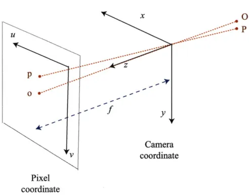
2-1 Illustration of the image formation using perspective projection of a pinhole camera. A 3D world point P is projected onto a 2D image

point p... 30

2-2 A thin-lens system. The lens' diameter is A and its focal length is f. The image plane is at distance fD from the lens and the focus distance is D. Rays from a point at distance S generates a circle of confusion diameter c. And the rays generates a virtual blur circle

diameter C at the focus distance D. . ... 31

2-3 This plot shows how the circle of confusion diameter, c, changes according to the change of object distance S and f-number N. c in-creases as a point is away from the focus distance D. The focus

distance D is 200cm, and the focal length f is 8.5cm . ... 32

2-4 View cameras and its movement of the standard front rise. (Images

from w ikipedia.) ... 33

2-5 Effect of rising front. The lens is moved vertically up along the lens plane in order to change the portion of the image that will be cap-tured on the film. As a result of rise, the principal point is not lo-cated at the image center, but at the bottom of the image. (Images

from The Camera [1] by Adams) ... 34

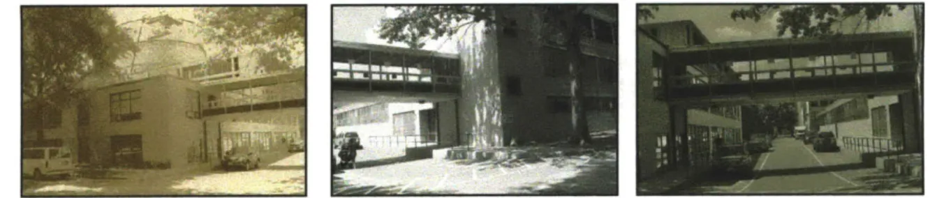
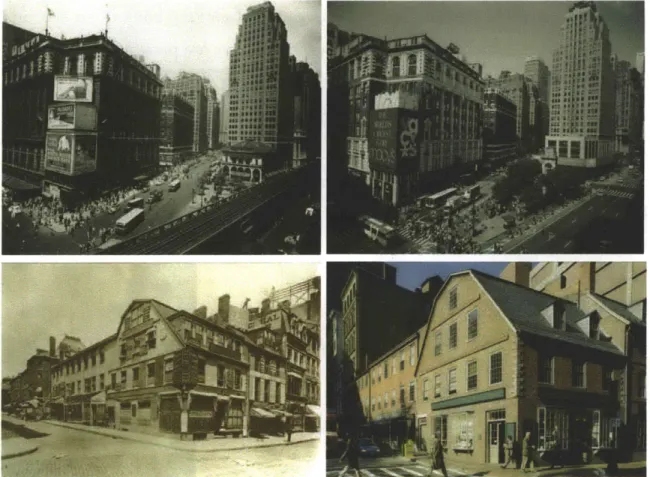
2-6 Rephotography gives two views of the same place around a century apart. Pictures are from New York Changing [2] and Boston Then

2-7 Ansel Adams using a dodging tool (from The Print [4] by Adams). He locally controls the amount of light reaching the photographic paper. . . . 37 2-8 Typical model photographs that we use. Photo (a) exhibits strong

contrast with rich blacks, and large textured areas. Photo (b) has

mid-tones and vivid texture over the entire image. . ... 38

4-1 In our prototype implementation, a laptop is connected to a cam-era. The laptop computes the relative camera pose and visualizes how to translate the camera with two 2D arrows. Our alignment

visualization allows users to confirm the viewpoint. . ... 46

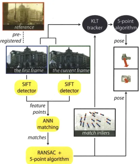
4-2 Overview of our full pipeline. In a preprocess, we register the ref-erence camera to the first frame. In our main process, we use an interleaved strategy where a lightweight estimation is refreshed pe-riodically by a robust estimation to achieve both real-time perfor-mance and robustness. Yellow rounded rectangles represent robust estimation and purple ellipses are for lightweight estimation. The robust estimation passes match inliers to the lightweight estimation

at the end. ... ... ... 49

4-3 Preprocessing to register the reference camera. . ... . 50

4-4 How to take the first photo rotated from where a user guesses to be

the desired viewpoint. ... 52

4-5 Under perspective projection, parallel lines in space appear to meet at the vanishing point in the image plane. Given the vanishing points of three orthogonal directions, the principal point is located at the orthocenter of the triangle with vertices the vanishing points 54 4-6 The synthetic cube images we used to test the accuracy of our

es-timation of principal point and camera pose. The left cube image (a) has its principal point at the image center, while the right cube image (b) moved its principal point to the image bottom. ... .54

4-7 Our interleaved pipeline. Our robust estimation and lightweight estimation are interleaved using three threads: one communicates with the camera, the other conducts our robust estimation, and an-other performs our lightweight estimation. At the end of each ro-bust estimation, a set of inliers is passed to the lightweight esti-mation thread. Numbers in this figure indicate the camera frame numbers. Note that for simplicity, this figure shows fewer frames

processed per robust estimation. . ... . .. 60

4-8 The flow chart of our interleaved scheme. . ... 61

4-9 The screen capture of our visualization. It includes two 2D arrows and an edge visualization. The primary visualization is the two 2D arrows. The top arrow is the direction seen from the top view and the bottom arrow is perpendicular to the optical axis. An edge visu-alization is next to the arrow window. The user can confirm that he has reached the desired viewpoint when the edges extracted from the reference are aligned with the rephoto result in our edge visual-ization. We show a linear blend of the edges of the reference image

and the current scene after homography warping. . ... 62

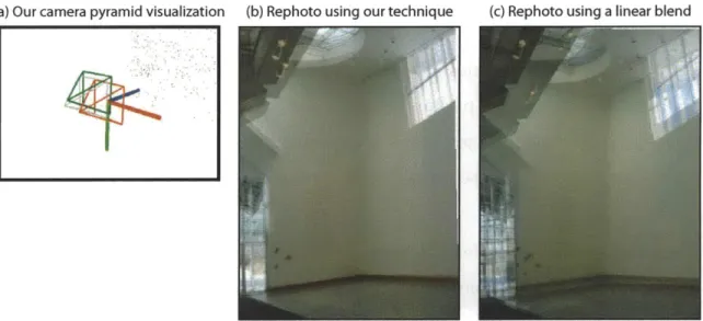
4-10 User study results with our first visualization. We displayed the rel-ative camera pose using 3D camera pyramids (a). The red pyramid showed the reference camera, and the green one was for the current camera. Although the rephoto using our technique (b) was better than that using a linear-blend (c), neither helped users to take

accu-rate rephotos. ... 66

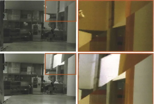
4-11 User study results in the indoor scenes. Split comparison between the reference image and users' rephotos after homography warping. The result at the top is from a user using our method, and the one at the bottom is from a user using a linear blend visualization. Notice

4-12 In the final user study, the reference photos had old-looking

appear-ances . ... ... .. . . 69

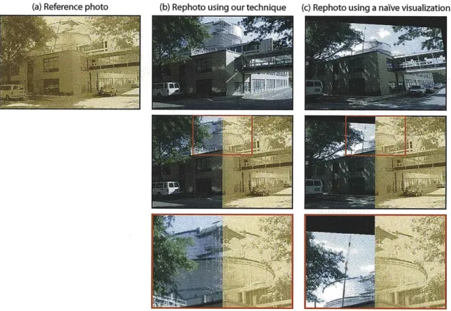
4-13 User study results. Left to right: (a) the reference photo and users' rephotos using our technique (b) and a naive visualization (c) af-ter homography warping. The second row show split comparison between the reference image and users' rephotos, and the last row has their zoomed-in. With our method, users took more accurate

rephotos... ... 70

4-14 User study results. Left to right: (a) the reference photo and users' rephotos using our technique (b) and a naive visualization (c) after homography warping. The last row shows two times zoomed-in blend of rephotos and outline features from (a) in red. The outline features from (a) match outline features in (b) but not in (c). This shows that users take more accurate rephotos using our technique

than using a naive visualization . ... . . . . .. . . 71

4-15 Results. Left to right: the reference images, our rephoto results, and professional manual rephotos without our method. This shows the

accuracy of our results. ... ... 72

4-16 Results. Left to right: the reference images, our rephoto results, three times zoomed-in blend of (b) and outline features from (a) in red. The outline features from (a) match outline features in (b). This

shows the accuracy of our results. ... . 73

4-17 Results. Left to right: the reference photos, our rephoto result, split comparison between the reference and our rephoto. This shows that

our technique enables users to take a faithful rephoto ... . 75

4-18 Results with style transfer. Left to right: the reference photos, our rephoto results, and our rephotos with styles transferred from the

reference photos. ... 76

5-1 The normalized average amplitude across scales: on the left is the low frequency and the right is the high frequency. (a) The aver-age amplitude in casual photographs is uniformly distributed across frequencies. (b) The average amplitude in the artistic photographs shows a unique distribution with a U shape or a high slope.) . . . . 80 5-2 The local spectral signatures show non-stationarity. The local

spec-tral signatures are obtained by taking normalized spectrum of each window : each amplitude is multiplied by its frequency. The degree of the non-stationarity varies in different images. The color close to red means a high value and that close to blue means a low value. . . 82 5-3 Overview of our pipeline. The input image is first split into base and

detail layers using bilateral filtering. We use these layers to enforce statistics on low and high frequencies. To evaluate the texture de-gree of the image, we introduce the notion of textureness. The layers are then recombined and post-processed to produce the final output.

The model is Kenro Izu's masterpiece shown in Figure 2-8b. ... 83

5-4 The output of the Gaussian blur contains low frequency contents, and the residual has high frequency components. However, this lin-ear filtering results in haloes and artifacts around edges. In contrast, the output of the bilateral filter (base) and its residual (detail)

pre-serve the edge information. ... 84

5-5 The bilateral filter can cause gradient reversals in the detail layer near smooth edges. Note the problems in the highlights (b). We force the detail gradient to have the same orientation as the input (c). Contrast is increased in (b) and (c) for clarity. . ... 87 5-6 Histogram matching. The remapping curve is deduces from the

in-put and model base histograms. Each pixel is transformed accord-ing to the remappaccord-ing curve. For the remappaccord-ing curve, the horizon-tal axis is the luminance of the input base. The vertical axis is the

5-7 Because of the preserved edges, the high frequencies of an image (b) appear both in the base layer (c) and in the detail layer (d). This phenomenon has to be taken into account to achieve an appropriate

analysis. ... 89

5-8 Textureness of a 1D signal. To estimate the textureness of the in-put (a), we comin-pute the high frequencies (b) and their absolute val-ues (c) . Finally, we locally average these amplitudes: Previous work based on low-pass filter (d) incurs halos (Fig. 5-9) whereas our cross

bilateral filtering yields almost no halos (e) . ... 90

5-9 Using a Gaussian filter to locally average the high frequency ampli-tudes yields halos around strong edges. To prevent this defect, we

use an edge-preserving filter. ... 91

5-10 Our measure of textureness indicates the regions with the most

con-trasted texture. ... 91

5-11 Without constraints, the result may lose valuable details (b) because the highlight are saturated. Enforcing the model histogram brings back the intensity values within the visible range (c). Finally, con-straining the gradients to preserve some of the original variations (a)

produces high quality details (d). ... . .. 92

5-12 Our system can seamlessly handle HDR images . We can turn a sharp picture (b) into a soft grainy and toned photograph (d). We have toned the histogram-transferred version (c) to prevent biased comparison due to different color cast. The model (a) is Accident at the Gare Montparnasse from the Studio Levy and Sons, 1895. The

input (b) is courtesy of Paul Debevec, USC . ... 96

5-13 Results from lower resolution (a) provides quick previews and al-low for interactive adjustments before rendering high resolution re-sults (b). Limited differences are visible on the smallest details (e.g.

in the background) because they are not well sampled in the

5-14 This rendition was obtained in two steps. We first used Kenro Izu's picture shown in Figure 2-8b as a model (b). Then, we manually increased the brightness and softened the texture to achieve the final rendition (c) that we felt is more suitable for the scene. . ... 97

5-15 A simple histogram matching from the model (a) to the input (b) increases the texture level of the image (c) whereas the model has little texture. In comparison, we successfully reduce the texture and the sharpness to achieve large uniform gray regions similar to those in the model. The model is Snapshot by Alfred Stieglitz. . ... 98

5-16 Histogram and frequency comparison. Our result (c) faithfully trans-fers local contrast from the model photo (b). In contrast, a direct histogram matching (d) increases the high frequency contents by spreading the luminance values. In the local spectral signatures, the color close to red means a high value and that close to blue means a

low value. ... 99

5-17 Our approach is able to reproduce the level of texture observed in Adams' masterpiece (a) to achieve a compelling rendition (d). In comparison, Adobe@ Photoshop@ "auto-level" tool spans the im-age histogram on the whole intensity range. This reveals the small features of a picture but offers no control over the image look (b). And, a direct histogram transfer only adjusts the overall contrast and ignores the texture, thereby producing a dull rendition (c). . . . 100

5-18 Histogram and frequency comparison. A direct histogram match-ing (d) increases the high frequency contents by spreadmatch-ing the lumi-nance values, but not as much as our result (c). In the local spectral signatures, the color close to red means a high value and that close

5-19 For color images, we process the luminance channel of the image and keep the original chrominance channels. In this example, the details are enhanced while the overall contrast and sharpness are increased. We used Adams' picture (Fig. 5-17a) as a model. ... . 102 5-20 Our technique suffers from imperfections such as JPEG artifacts. In

this example, the artifacts in the sky are not visible in the input im-age (Fig. 5-10a) but appear clearly after processing. ... 102 6-1 Our technique magnifies defocus given a single image. Our defocus

map characterizes blurriness at edges. This enables shallow depth of field effects by magnifying existing defocus. The input photo was taken by a Canon PowerShot A80, a point-and-shoot camera with a sensor size of 7.18 x 5.32 mm, and a 7.8 mm lens at f/2.8. ... 106 6-2 Given the same field of view and the same f-number (f/2.8), a large

sensor (a) yields more defocus than a small sensor (b) does. ... 106 6-3 The model for the distance between second-derivative extrema. We

numerically fit this response model with various d around the edge pixel and along the gradient direction to find the distance d with a

least square fitting error ... 111

6-4 The zero-crossing of the third derivative (c) is greatly affected by neighboring edges and cannot localize the second derivative ex-trema. In contrast, our approach (d) can estimate the blur sigma that is close to the actual blur sigma (b). The input (a) is generated using the blur sigma (b). In the blur measure, the color close to red

means blurry and that close to blue means sharp. ... . . 112

6-5 Blur measure before and after the cross bilateral filtering. The cross bilateral filtering refines outliers such as yellow and green measures (b), which mean blurry, in the focused regions to be blue measures (c), which means sharp. The blur measures are downsampled using

6-6 Defocus map with various a. a controls the balance between the smoothness penalty term and data term in Equation 6.7. We use a = 0.5 for edge pixels and a = 0 for non-edge pixels, which do not have values. In this plot, red means blurry region and blue means

sharp regions. The input image is Figure 6-5. . ... . 115

6-7 Results. The original images, their defocus maps, and results blurred using our approach. The inputs were taken by (a) a Nikon D50 with a sensor size of 23.7 x 15.6 mm and a 180.0 mm lens at f/4.8, (b) a Canon 1D Mark II with a sensor size of 28.7 x 19.1 mm and a Canon EF 85mm f/1.2L lens, and (c, d) a Canon PowerShot A80, a point-and-shoot camera with a sensor size of 7.18 x 5.32 mm, and a 7.8 mm lens at f/2.8. The two at the bottom are from bigfoto.com. .... 118 6-8 Doubled defocus. Doubling the defocus map generates a effect of

doubling the aperture size. As we double the defocus map (c) of the f/8 image, we obtain a result similar to the defocus map (d) of the f/4 image. While the simulated defocused map (e) is not exactly the same as the real map (d), the output image with magnified defocus

(f) is visually close to the f/4 photograph (b). . . . ... 119 6-9 Using our defocus map, we can synthesize refocusing effects. We

perform deconvolution using our defocus map (b) and apply lens blur. The result (c) looks as if the foreground is focused. The in-put photo was taken by a Canon PowerShot A80, a point-and-shoot camera with a sensor size of 7.18 x 5.32 mm, and a 7.8 mm lens at f/2.8. . . . ... . . . 119

List of Tables

4.1 Analysis of the robustness of our estimation against the user input error. Small errors show that our principal point estimation is robust

against the user input error. ... . 55

4.2 Our principal point constraint using vanishing point estimation

en-ables an accurate estimation of the viewpoint. ... 56

4.3 User study errors. With our method, users made less than 8 % of error than with a linear blend. The P-value is smaller than 0.05. This means that this result is statistically meaningful and significant. . . . 67 4.4 User study errors. The error with a linear blend is 2.5 times larger

Chapter 1

Introduction

A good snapshot stops a moment from running away. -Eudora Welty (1909-2001)

Photography is a medium of discovery and documentation. Every photograph has its own purpose. Landscape photographs are to capture magnificent sceneries. Artistic landscape photographs evoke emotion and carry the viewer away to the breathtaking beautiful sceneries. Snapshots are to record memorable moments. Good snapshots are tangible reminders that bring the past experience and moment into the present. In addition, photographs can be used to document changes. For example, a photograph taken at the same location many years later can emphasize change over time. This is called re-photography. Rephotographs are to visualize historic continuities and changes. When a photograph and its rephotograph match well, it becomes very evident what is preserved and what changed across time.

Digital technologies have made photography less expensive and more accessi-ble. Still, casual photographers are often disappointed with their photos that are different from what they thought to capture. Landscape photos lack contrast and strength. Portrait photos are not correctly focused or have distracting background clutter. The viewpoint of the rephoto could be reproduced better at capture time. The framing and composition could have been done better.

knowledge, and persistence. Photographers need to carefully choose the subject and composition of a picture, to select the right lens and viewpoint, and to make great efforts with lighting and post-processing to arrange the tones and contrast. Unfortunately, such painstaking work and advanced skill is out of reach for ca-sual photographers. In addition, for professional photographers, it is important to improve workflow efficiency.

Advanced computer vision techniques embedded in recent digital cameras, such as face detection and viewfinder alignment [5], help focus on the right sub-ject and change framing but do not address viewpoint and composition. Software such as Apple's Aperture and Adobe's Lightroom focuses on workflow optimiza-tion but offers little interactive editing capabilities.

The goal of our work is to allow users to achieve a faithful viewpoint for repho-tography and a particular appearance with ease and speed. To this end, we analyze and transfer properties of a model photo to a new photo. In particular, we trans-fer the viewpoint of a retrans-ference photo to enable rephotography. In addition, we transfer photographic appearance from a model photo to a new input photo.

1.1 Overview of Our Approach

In this thesis, we present two contributions that transfer photographic view and look using model photographs and one contribution that magnifies existing de-focus given a single photo. In "Computational Re-Photography", we address the challenge of viewpoint matching for rephotography. Our interactive, computer-vision-based technique helps users match the viewpoint of a reference photograph at capture time. Our technique estimates and visualizes the camera motion re-quired to reach the desired viewpoint. In "Style Transfer", we focus on the tonal aspects of photographic look using post-processing. We decouple the tonal aspects of photos from their contents. Our method handles global and local contrast sepa-rately. In "Defocus Magnification", we magnify defocus given a single image. We analyze the existing defocus in the input image and increase the amount of defocus

present in out-of focus regions. Let us describe them more in details below.

1.1.1

Computational Re-Photography

Our real-time interactive technique helps users reach a desired viewpoint and lo-cation as indicated by a reference image. This work is inspired by rephotography, the act of repeat photography of the same site. Rephotographers aim to recapture an existing photograph from the same viewpoint. However, we found that most rephotography work is imprecise because reproducing the viewpoint of the orig-inal photograph is challenging. The rephotographer must disambiguate between the six degrees of freedom of 3D translation and rotation, and the confounding similarity between the effects of camera zoom and dolly.

The main contribution of our work is the development of the first interactive, computer-vision-based technique for viewpoint guidance. We envision our tool running directly on the digital camera. However, since these platforms are cur-rently closed and do not have enough processing power yet, our prototype consists of a digital camera connected to and controlled by a laptop. At capture time, users do not need to examine parallax manually, but only need to follow our real-time visualization displayed on a computer in order to move to a specific viewpoint and location. The user simply captures a video stream of the scene depicted in the reference image, and our technique automatically estimates the viewpoint and lens difference and guides users to the desired viewpoint. Our technique builds on several existing computer vision algorithms to detect and match common features in two photographs [6] and to compute the relative pose between them [7, 8]. We demonstrate the success of our technique by rephotographing historical images and conducting user studies. We envision that this work would enable cameras to become more interactive and embed more computation.

1.1.2

Style Transfer

Our technique transfers the tonal aspect of photographic look from a model pho-tograph onto an input one. We handle global and local contrast separately. Our method is inspired by traditional photography, where the darkroom offers remark-able global and local control over the brightness, contrast, and sharpness of images via a combination of chemical and optical processes [4, 9].

Our method is based on a two-scale non-linear decomposition of an image. We modify different layers according to their histograms. To transfer the spatial variation of local contrast, we introduce a new edge-preserving textureness that measures the amount of local contrast. We recombine the two layers using a con-strained Poisson reconstruction. Finally, additional effects such as soft focus, grain and toning complete our look transfer.

1.1.3

Defocus Magnification

We take a single input image that lacks defocus and increase the amount of defocus present in out-of focus regions. A blurry background due to shallow depth of field is often desired for photographs such as portraits, but, unfortunately, small point-and-shoot cameras do not permit enough defocus because of the small diameter of their lenses and their small sensors. We present an image-processing technique that increases the defocus in an image and simulates the shallow depth of field of a lens with a larger aperture.

Our technique estimates the spatially-varying amount of blur over the image, and then uses a simple image-based technique to increase defocus. We first es-timate the size of the blur kernel at edges and then propagate this defocus mea-sure over the image. Using our defocus map, we magnify the existing blurriness, which means that we blur blurry regions and keep sharp regions sharp. In contrast to more difficult problems such as depth from defocus, we do not require precise depth estimation and do not need to disambiguate textureless regions.

---1.2 Thesis Overview

This thesis addresses analysis and transfer of photographic viewpoint and pearance. Given a model photo, we transfer its photographic viewpoint and ap-pearance to an input photo. Chapter 2 introduces some background information that inspired this thesis. We provide a brief overview on traditional photogra-phy. Chapter 3 discusses previous work that addresses computer vision and com-puter graphics challenges related to our goal. Chapter 4 presents our viewpoint guidance technique. We describe our method and demonstrate the success of our technique by presenting rephotography results and user study results. Chapter 5 presents our two-scale tone transfer method. We perform a faithful reproduction of the tonal aspects of model photographs. Chapter 6 shows our defocus magnifi-cation technique. Our image-processing technique simulates the shallow depth of field effects. Chapter 7 summarizes our work and discusses our future work.

Chapter 2

Background

Our techniques are inspired by and related to traditional photography. This chap-ter provides a brief overview on camera models including the pinhole camera, lens camera, and view camera, photographic printing, and rephotography.

2.1

Camera Models and Geometric Image Formation

In this section, we review some of the basic camera models related to our tech-nique. First, we describe the geometric image formation by a pinhole camera. Sec-ond, we examine a lens camera and the amount of defocus. Finally, we discuss a view camera and its rising front adjustment.

2.1.1

Pinhole Camera and Perspective Projection

Most computer vision algorithms assume perspective projection formed by a pin-hole camera. The pinpin-hole camera is the simplest camera model. It maps 3D onto 2D using perspective projection. Rays of light pass through a pinhole and form an inverted image of the object on the image plane, as shown in Figure 2-1.

Using homogeneous coordinates allows projection to be a matrix multiplica-tion, as shown in Equation 2.1. K is a 3 x 3 intrinsic matrix that maps the 3D camera coordinate to the 2D pixel coordinate in homogeneous coordinates.

Equa-x _O p *..-.- - --~ Camera v coordinate Pixel coordinate

Figure 2-1: Illustration of the image formation using perspective projection of a pinhole camera. A 3D world point P is projected onto a 2D image point p.

tion 2.2 shows that K has five degrees of freedom including skew s, focal length

fv,

fs/f,.

V =- 0 (2.1) z _z 1

fs

UO

fV

2.1.2

Lens Camera and Defocus

In the pinhole camera, a smaller pinhole generally results in sharper images. How-ever, due to the wave properties of light, an extremely small hole can produce diffraction effects and a less clear image. In addition, with a small pinhole, a long exposure is required to generate a bright image. A lens replaces the pinhole to fo-cus the bundle of rays from each scene point onto the corresponding point in the image plane. This substitution makes the image brighter and sharper. Although most camera lenses use more intricate designs with multiple lens elements, here we review the simplified thin lens model, which suffices in our context.

The main role of a lens is to make all the rays coming from a point at the focus distance converge to a point in the image plane. In contrast, the rays originating at a scene point distant from the focus distance converge in front of or behind the im-age plane, and that point appears as a blurred spot in the imim-age. The blurred spot is called the circle of confusion. It is not strictly speaking a circle and depends on the aperture shape and diffraction, but it is often modeled as a circle or a Gaussian. We express the circle of confusion diameter c of a point at distance S (Figure 2-2). A detailed derivation can be found in optics textbooks such as Hecht's [10]. Given the focal length f of the lens, the thin-lens formula gives us the lens-sensor distance fD to focus at distance D: 1 = 1 + .

A X

D _{> f}

S - AD

Figure 2-2: A thin-lens system. The lens' diameter is A and its focal length is f. The image plane is at distance fD from the lens and the focus distance is D. Rays from a point at distance S generates a circle of confusion diameter c. And the rays generates a virtual blur circle diameter C at the focus distance D.

The f-number N gives the aperture diameter A as a fraction of the focal length

(A = N

f).

phers set to control the diaphragm. The aperture is then denoted by, e.g., f/2.8 to express that the diameter is the focal length divided by the f-number. The diameter of the circle of confusion is then

IS - D

_f2

Figure 2-3: This plot shows how the circle of confusion diameter, c, changes ac-cording to the change of object distance S and f-number N. c increases as a point is away from the focus distance D. The focus distance D is 200cm, and the focal length f is 8.5cm

Figure 2-3 shows that the circle of confusion diameter c increases as a point is away from the focus distance D. The relationship is not linear (hyperbolic) and is not symmetrical for points in front of and behind the plane in focus.

We now study the effect of the sensor size, X. To express the amount of defocus in terms of image-space blur, we use the relative size of the circle of confusion c' = c/X. For sensors of different sizes, the same field of view is obtained if the relative focal length f' = f/X is the same. Replacing c and f by their relative version in Eq. 2.3 we obtain

S- D f'2X

S N(D - f'X) _(2.4)

To a first-order approximation, the amount of defocus is proportional to the sensor size X. This confirms that for a given f-number N, a smaller sensor does

not yield as much defocus as a larger sensor. More defocus could be achieved by using a smaller f-number (larger lens aperture), but this would require bending rays that reach the periphery of the lens aperture by angles that are physically challenging to achieve. Scaling down the sensor and lens inherently scales down the amount of defocus. In this thesis, we synthesize the shallow depth of field effect by increasing the amount of defocus existing in an input image using image processing techniques.

2.1.3

View Camera and Principal Point

The view camera is the most versatile of the large-format cameras. Historical pho-tographs were often taken with view cameras. The view camera comprises a flex-ible bellows, which allow photographers to control focus and convergence of par-allel lines by varying the distance between the lens and the film over a large range. Figure 2-4 illustrates a view camera.

Fimn Plane Lens Plane

Frnt Stadrd

Lou Axis

Figure 2-4: View cameras and its movement of the standard front rise. (Images from wikipedia.)

In particular, the rising front adjustment is a very important movement espe-cially in architectural photography. The lens is moved vertically up along the lens plane in order to change the portion of the image that will be captured on the film. Figure 2-5 demonstrates the effect of rising front. The main effect of rise is to eliminate converging parallels when photographing tall buildings. If a camera is pointed at a tall building without rise movement nor tilt, the top will be cut off. If

the camera is tilted upwards to get it all in, the film plane will not be parallel to the building, and the top of the building will appear narrower than its bottom. That is, parallel lines in the object will converge in the image.

Figure 2-5: Effect of rising front. The lens is moved vertically up along the lens plane in order to change the portion of the image that will be captured on the film. As a result of rise, the principal point is not located at the image center; but at the bottom of the image. (Images from The Camera [1] by Adams)

The principal point is the intersection of the optical axis with the image plane. As a result of rise, the principal point does not locate at the image center, but at the image bottom. When we estimate the viewpoint of the reference photo, we estimate the location of the principal point as preprocessing.

2.2

Rephotography

Rephotography is the act of repeat photography; capturing a photograph of the same scene from the same viewpoint of an existing photograph typically much older. Figure 2-6 shows two examples. A photograph and its rephotograph can provide a compelling "then and now" visualization of the progress of time. When a photograph and its rephotograph match well, a digital cross-fade between the two is a remarkable artifact. A hundred years go by in the blink of an eye, and it becomes immediately evident which scene elements are preserved across time, and which have changed.

However, precise rephotography requires a careful study of the viewpoint, lens, season, and framing of the original image. Exactly matching a photograph's viewpoint "by eye" is remarkably challenging. The rephotographer must disam-biguate between the six degrees of freedom of 3D translation and rotation, and the confounding similarity between the effects of camera zoom and dolly. Our viewpoint visualization technique automatically estimates the lens and viewpoint differences. Users only need to follow our real-time visualization in order to move to a specific viewpoint and location instead of manually examining parallax.

2.3 Traditional Photographic Printing

Photographic printing is the process of producing a final image on paper. Tradi-tional photographic printing is performed in a photographic darkroom. The dark-room offers remarkable global and local control over the brightness, contrast, and sharpness of images via a combination of chemical and optical processes [9, 4]. As a result, black-and-white photographs vary in their tonal palette and range. Pho-tographers like Adams (Fig. 2-8a) exhibit strong contrast with rich blacks, while artists like Stieglitz (Fig. 5-15a) rely more on the mid-tones. This suggests the in-tensity histogram as a characterization of tonal look.

Y

. . . .

Figure 2-6: Rephotography gives two views of the same place around a century apart. Pictures are from New York Changing [2] and Boston Then and Now [3].

Figure 2-7: Ansel Adams using a dodging tool (from The Print [4] by Adams). He locally controls the amount of light reaching the photographic paper.

account because a histogram does not deal with local contrast. The amount of texture is crucial in photographs; some artists use vivid texture over the entire image (Fig. 2-8b), while others contrast large smooth areas with strong textures in the remaining parts of the image (Fig. 2-8a). Furthermore, the human visual system is known to be more sensitive to local contrast than to low spatial frequencies. Finally, a photograph is characterized by low-level aspects of the medium such as tone (e.g. sepia toning) and grain (controlled by the film and paper characteristics). These observations drive our approach. We use decompositions of an image that afford direct control over dynamic range, tonal distribution, texture and sharpness.

(a)

(b)

Figure 2-8: Typical model photographs that we use. Photo (a) exhibits strong con-trast with rich blacks, and large textured areas. Photo (b) has mid-tones and vivid texture over the entire image.

Chapter 3

Related Work

Computational photography extends the capabilities of digital photography. This thesis focus on transfer of photographic characteristics including viewpoint, tonal aspects, and defocus. In this chapter, we review previous work that addresses related challenges.

3.1 Viewpoint Estimation

To the best of our knowledge, we are the first to build an interactive tool that directs a person to the viewpoint of a reference photograph. However, estimating camera positions and scene structures from multiple images has been a core problem in

the computer vision community [11, 12, 8, 13].

We visualize the desired movement at capture time. One alternative to our approach is to capture a nearby viewpoint and warp it to the desired viewpoint after capture [14, 15, 16]. However, parallax and complex scene geometry can be challenging for these algorithms, and the result would be inaccurate.

Our technique is related to visual homing research in robotics, where a robot is directed to a desired 3D location (e.g., a charging station) specified by a pho-tograph captured from that location. The visual homing approach of Basri et al. [17] also exploits feature matches to extract relative pose; the primary difference is that robots can respond to precise motion parameters, while humans respond

better to visualizations in a trial and error process. More recent work exists on real-time algorithms that recover 3D motion and structure [18, 19], but they do not aim to guide humans. There exist augmented reality systems [20] that ease navi-gation. However they assume that the 3D model is given, while the only input to our technique is an old photograph taken by an unknown camera.

We are not the first to exploit the power of historical photographs. The 4D Cities project (www.cc.gatech.edu/4d-cities) hopes to build a time-varying 3D model of cities, and Photo Tourism [21] situated older photographs in the spatial context of newer ones. However, neither project helps a user capture a new photograph from the viewpoint of a historical one.

Real-time visualization on a camera allows photographers to achieve a variety of tasks. It helps photographers focus on the right subject and change framing and settings. In addition to the traditional simple functions, advanced computer vi-sion techniques have been embedded in recent digital cameras and mobile phones. Face detection, the Viewfinder Alignment of Adams et al. [5], feature matching and tracking on mobile phones [22, 23], and the Panoramic Viewfinder of Baud-isch et al. [24] are such examples. The Panoramic Viewfinder is related to our technique, though its focus is the real-time preview of the coverage of a panorama with no parallax. The implementation of matching and tracking algorithms on mobile phones is complementary to our technique. We focus on the development of an interactive visualization method based on those tools.

3.2 Style Transfer

The frequency contents have been used to measure statistical characteristics of nat-ural images. Field investigated the two-dimensional amplitude spectra and found regularity among natural images that the average amplitude falls as [25]. This property is called scale invariance [26]. We observe that natural images fol-low such scale invariant property, while artistic photographs do not show such invariance. In addition to the scale invariance, image statistics have been shown to

be non-stationary [27]: local statistical features vary with spatial location. In this thesis, we use the scale variance and the variations in non-stationarity to analyze and transfer photographic styles.

Tone-mapping seeks the faithful reproduction of high-dynamic-range images on low-dynamic-range displays, while preserving visually important features [28]. Our work builds on local tone mapping where the mapping varies according to the neighborhood of a pixel [29, 30, 31, 32, 33, 34]. The precise characteristics of film have also been reproduced [35, 31]. However, most techniques seek an objective rendering of the input, while we want to facilitate the exploration and transfer of particular pictorial looks.

Style transfer has been explored for the textural aspects of non-photorealistic media, e.g. [36, 37], and DeCarlo et al. stylize photographs based on saliency [38]. In contrast, we seek to retain photorealism and control large-scale effects such as tonal balance and the variation of local detail. In addition, our paramet-ric approach leads to continuous changes supported by interactive feedback and enables interpolations and extrapolations of image look.

Our work is inspired by the ubiquitous visual equalizer of sound devices. Sim-ilarly, the modification of frequency bands can alter the "mood" or "style" of mo-tion data [39]. The equivalent for images is challenging because of the halos that frequency decomposition can generate around edges. Our work can be seen as a two-band equalizer for images that uses non-linear signal processing to avoid halos and provides fine tonal and spatial control over each band.

Recently manual adjustment tools [40, 41] are developed and multiscale edge-preserving decomposition schemes [42, 43] are introduced. There are complemen-tary to our technique. We aim to transfer photographic looks from model pho-tographs.

3.3 Defocus

Defocus effects have been an interest of the Computer Vision community in the context of recovering 3D from 2D. Camera focus and defocus have been used to reconstruct depth or 3D scenes from multiple images: depth from focus [44, 45, 46, 47, 48] and depth of defocus [49, 46, 50, 51, 52, 53]. These methods use multiple images with different focus settings and estimate the corresponding depth for each pixel. They have to know the focus distance and focal length to computer the depth map. In contrast, we do not estimate the depth but the blur kernel. Recently, specially designed cameras [54, 55, 56] are introduced to infer depth or blur kernel after the picture has been taken. We want to treat this problem without the help of any special camera settings, but only with image post-processing techniques.

Image processing methods have been introduced to modify defocus effects without reconstructing depth. Eltoukhy and Kavusi [57] use multiple photos with different focus settings and fuse them to produce an image with extended depth of field. Ozkan et al. [58] and Trussell and Fogel [59] have developed a system to restore space-varying blurred images and Reeves and Mersereau [60] find a blur model to restore blurred images. This is the opposite of what we want to do. They want to restore blurred images, while we want to increase existing blurriness.

Kubota and Aizawa [61] use linear filters to reconstruct arbitrarily focused im-ages from two differently focused imim-ages. On the contrary, we want to modify defocus effects only with a single image. Lai et al. [62] use a single image to esti-mate the defocus kernel and corresponding depth. But their method only works on an image composed of straight lines at a spatially fixed depth.

Given an image with a corresponding depth map, depth of field can be approx-imated using a spatially-varying blur, e.g. [63, 64], but note that special attention must be paid to occlusion boundaries [65]. Similar techniques are now available in commercial software such as Adobe@ Photoshop@ (lens blur) and Depth of Field Generator Pro (dofpro.com). In our work we simply use these features and instead of providing a depth map, we provide a blurriness map estimated from the photo.

While the amount of blurriness is only related to depth and is not strictly the same as depth, we have found that the results qualitatively achieve the desired effect and correctly increase defocus where appropriate. Note that a simple remapping of blurriness would yield a map that resembles more closely a depth map.

Chapter 4

Computational Re-Photography

This work seeks to facilitate rephotography, the act of repeat photography of the same site. Rephotographers aim to recapture an existing photograph from the same viewpoint. However, we found that most rephotography work is impre-cise and tedious because reproducing the viewpoint of the original photograph is challenging. The rephotographer must disambiguate between the six degrees of freedom of 3D translation and rotation, and the confounding similarity between the effects of camera zoom and dolly.

Our real-time interactive technique helps users reach a desired viewpoint and location as indicated by a reference image. In a pilot user study, we observed that people could not estimate depth by examining parallax. In our second user study, we showed the relative viewpoint information in 3D. Users found it hard to interpret 3D information; most had a hard time separating translation and rotation of the camera. The main contribution of our work is the development of the first interactive, computer-vision based visual guidance technique for human motion. Users only need to follow our real-time visualization displayed on a computer in order to move to a specific viewpoint and location instead of manually examining parallax.

4.1 Overview

Figure 4-1: In our prototype implementation, a laptop is connected to a camera. The laptop computes the relative camera pose and visualizes how to translate the camera with two 2D arrows. Our alignment visualization allows users to confirm the viewpoint.

Ultimately we wish to embed the whole computation onto the camera, but our current implementation has a laptop connected to a camera as shown in Figure 4-1 shows. The camera's viewfinder images are streamed out to the laptop. The laptop computes the relative camera pose and visualizes the direction to move the camera. We give an overview of how users interact with our technique and how we estimate and visualize the direction to move.

4.1.1

User interaction

We have realized an informal pilot user study to understand the challenges of rephotography. We found that users have much difficulty judging parallax and the effect of viewpoint change. In addition, they are confused by the number of de-grees of freedom: camera translation, rotation, and zoom. We have experimented a number of simple visualizations that combine the reference and current images to try to facilitate rephotography, including the difference image, a linear-blend composite, and side-by-side views. In all cases, users had difficulties interpreting the displays.

This motivates our approach, which seeks to minimize the number of degrees

of freedom that the user needs to control to translation only, and displays direct guidance in the form of arrows. We only provide an alignment visualization to help with the end game when the user is close enough to the desired viewpoint. Furthermore, this alignment visualization is made easier to interpret by compu-tationally solving for the extra degrees of freedom (rotation and zoom), automat-ically applying the appropriate homography warp to the current image to best match the reference.

Our approach takes as input a reference (old) image. We require the user to take a first pair of photographs of the scene from viewpoints that are distinct enough for calibration and that provide wide baseline to avoid degeneracies. In the case of an old reference photograph, the user clicks on a few correspondence points in those original images because the difference in appearance between old and new photos confuses even state-of-the art feature matching. Our interactive technique then automatically computes the difference between the current viewpoint and that of the reference photograph. It displays the required translation vector to guide the user, and refreshes several times per second. An alignment visualization between the reference and current images is also refreshed continuously. The automatic compensation for difference in orientation and zoom (within reason) allows the user to focus on parallax and the viewpoint itself.

4.1.2

Technical overview

To estimate and visualize the required translation, we leverage a number of computer-vision methods. In particular, we need to match features between images and

deduce relative camera pose in real time. To achieve both real-time performance and robustness, we use an interleaved strategy where a fast but simpler method is refreshed periodically by a more involved and more robust method. Our robust but slower estimation is based on SIFT matching [6] and a robust relative pose estimation based on RANSAC [66] and Stewenius's five-point algorithm [7]. Our lightweight estimation tracks the feature points estimated trustworthy by the

ro-bust process using simple tracking [67] and updates the relative pose accordingly. Figure 4-2 shows our full pipeline.

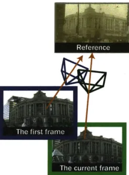
In addition to very different appearance of historical photos, their focal lengths and principal points are unknown; historical photographs of urban and architec-tural scenes were often taken with view cameras where the photographer would move the optical axis off center to keep verticals parallel while taking photographs from a low viewpoint. In a preprocess, we estimate the principal point and reg-ister the reference camera to the first frame. To this end, we triangulate feature points in the first pair of photographs into 3D points. Given a few correspondence points provided by the user, we compute the pose and focal length of the reference camera with respect to the known 3D points using the Levenberg-Marquardt (LM) nonlinear optimization algorithm [68, 69]. The resulting relative camera pose be-tween the first frame and the reference is used throughout our main estimation. In our main estimation, we estimate the camera pose relative to the first view instead of the reference. Since we know the reference camera location relative to the first-view, we can derive the relative pose between the current and reference photos.

pre- : registered -h rtfrm I SIFT detector I SIFT detector feature points ANN matching matchesI RANSAC + 5-point algorithm

e

Figure 4-2: Overview of our full pipeline. In a preprocess, we register the reference camera to the first frame. In our main process, we use an interleaved strategy where a lightweight estimation is refreshed periodically by a robust estimation to achieve both real-time performance and robustness. Yellow rounded rectangles represent robust estimation and purple ellipses are for lightweight estimation. The robust estimation passes match inliers to the lightweight estimation at the end.

... -... .... .... ... .... ;;...

P"Irlp

reference

I

4.2 Preprocess

feature points feature points

structure and pose

feature pointsl

Estimate structure

reeenefca ent seestutue+RI

!

A , "J "J I I

Figure 4-3: Preprocessing to register the reference camera.

At runtime, our system is given a reference image and a current frame and visualizes the translational component of the relative pose. However, there are four main challenges for viewpoint estimation for rephotography:

1. Historical images have very different appearance from current scenes be-cause of, e.g., architectural modifications, the film response, aging, weather and time of day changes. These dramatic differences challenge even state-of-the art feature descriptors. Comparing gradients and pixel values cannot find matches between old photographs and current scenes.

2. The focal length and principal point of the reference camera are unknown, and we have only one image.

3. The resulting translational component from camera pose estimation is unit-length due to scale ambiguities; the unit-length of the translational component is not meaningful across frames.

4. Rephotography seeks to minimize the translational component between the reference and the current. Unfortunately, pose estimation suffers from mo-tion degeneracy where there is no translamo-tion [?]. Even a narrow baseline results in unstable pose estimation. The baseline refers to the distance be-tween the camera centers.

To overcome these challenges, we use a wide-baseline 3D reconstruction. In pre-processing, we extract a 3D structure of the scene from the first two calibrated images using Structure from Motion (SfM) [13]. We calibrate the current cameras using the Camera Calibration Toolbox for Matlab [70]. With respect to the known 3D structure, we compute the pose and focal length of the old reference camera us-ing Levenberg-Marquardt (LM) nonlinear optimization. The input to the nonlinear optimization includes 2D-3D correspondences and an estimated principal point of the reference photo. In the case of an old reference photograph, we ask users to se-lect six to eight correct matches between the reference image and the second frame. We estimate the principal point of the reference image using its vanishing points. This preprocessing outputs the relative camera pose between the first frame and the reference, which will be used throughout our main estimation.

4.2.1 A wide-baseline 3D reconstruction

We reconstruct the 3D structure of the scene from the first and second view us-ing triangulation [13]. This 3D information is used to estimate the reference focal length and consistent scale over frames. For a wide-baseline 3D reconstruction, we require the user to take a first pair of photographs of the scene from viewpoints that are distinct enough. That is, we ask the user to take the first frame after ro-tating the camera 20 degrees around the main subject from the initial guess (See Fig 4-4.) The interactive process then starts from the second photo. Consequently, the baseline between the first view and the following frames and the baseline be-tween the first view and the desired viewpoint become wide. Using a first view guarantees wide enough baseline and improves the accuracy of the camera pose

algorithm.

Figure 4-4: How to take the first photo rotated from where a user guesses to be the desired viewpoint.

4.2.2

Reference camera registration

We relate the reference image to the reconstructed world from the first two photos taken by the user. Given matches between the reference and a current photo, we in-fer the intrinsic and extrinsic parameters of the rein-ference camera using Lourakis's LM package [71]. We assume that there is no skew. This leaves us nine degrees of freedom: one for the focal length, two for the principal point, three for rotation, and three for translation. We initialize the rotation matrix to be the identity matrix, the translation matrix to be zero, and the focal length to be the same as the current camera. We initialize the principal point by analyzing the vanishing points. We describe the details below.

Although this initialization is not close to the ground truth, we observe that the Levenberg-Marquardt algorithm converges to the correct answer since we allow only 9 degrees of freedom and the rotation matrix tends to be close to the identity matrix for rephotographying. The final input to the nonlinear optimization is a set

of matches between the reference and the first photo that users enter. Since we have already triangulated feature points in the first pair of photographs into 3D points, we know the 3D positions of the matched feature points. We compute the pose and focal length of the reference camera with respect to the known 3D locations. In addition, we re-project all 3D points from the first pair to the reference. These points are used to estimate the appropriate homography warp for our alignment visualization.

Principal point estimation

The principal point is the intersection of the optical axis with the image plane. If a shift movement is applied to preserve the verticals parallel or if the image is cropped, the principal point is not in the center of the image, and it must be computed. The analysis of vanishing points provides strong cues for inferring the location of the principal point. Under perspective projection, parallel lines in space appear to meet at a single point in the image plane. This point is the vanishing point of the lines, and it depends on the orientation of the lines. Given the vanishing points of three orthogonal directions, the principal point is located at the orthocenter of the triangle with vertices the vanishing points [13], as shown in Figure 4-5.

We ask the users to click on three parallel lines in the same direction; although two parallel lines are enough for computation, we ask for three to improve robust-ness. We compute the intersections of the parallel lines. We locate each vanishing point at the weighted average of three intersections. The weight is proportional to the angle between two lines [72]. We discard the vanishing point when the sum of the three angles is less than 5 degrees.

With three finite vanishing points, we initialize and constrain the principal point as the orthocenter. If we have one finite and two infinite vanishing points, we initialize and constrain the principal point as the finite vanishing point. With two finite vanishing points, we constrain the principal point to be on the vanishing line that connects the finite vanishing points.