Analyzing CMS open collider data through topic modeling

Analyzing CMS Open Collider Data through Topic Modeling

by

Radha Mastandrea

Submitted to the Department of Physics

in partial fulfillment of the requirements for the degree of

Bachelor of Science in Physics

at the

MASSACHUSETTS INSTITUTE OF TECHNOLOGY

June 2019

0 Massachusetts Institute of Technology 2019. All rights reserved.

Signature redacted

Department of Physics

May 9th, 2019

Certified by...

Signature redacted

Jesse Thaler

Associate Professor of Physics

Thesis Supervisor

Signature redacted

Nergis Mavalvala

Associate Department Head, Department of Physics

>i

Author ...

Accepted by ...

MASSACHU SCETS INSTITUTE O--F TECHNOLOGY

JUL 2

4

2019

LIBRARIES

Analyzing CMS Open Collider Data through Topic Modeling

by

Radha Mastandrea

Submitted to the Department of Physics on May 09, 2019, in partial fulfillment of the

requirements for the degree of Bachelor of Science in Physics

Abstract

We conduct an investigation of jet substructure at the Large Hadron Collider (LHC) on the CMS Open Data. We analyze a sample of jets detected by the CMS experiment in 2011 with the companion simulated (both pre- and post-detector) jet datasets to demonstrate the ability of our analysis framework to accurately quantify jet substructure observables as well as properly describe the effects of the CMS detector. We move to a specific analysis of jet classification using the unsupervised algorithm of jet topics to provide a new way of defining the categories of quark and gluon jets through their observable properties. We finally outline a means of accessing our sample of 883,431 high quality CMS-detected jets so that other scientists may conduct their own analyses on this sample.

Thesis Supervisor: Jesse Thaler Title: Associate Professor of Physics

4

Acknowledgments

The author thanks Preksha Naik, Patrick T. Komiske, Eric M. Metodiev, and Jesse Thaler for their substantial contributions to the research of this project and writing of the upcoming publication that this paper is based off. The author also thanks Maximilian Henderson, Edward Hirst, and Ziqi Zhou for their collaboration in the early stages of this work. The author gratefully acknowledges the Heising-Simons Foundation for their generous fellowship program that funded the many hard drives and computing resources needed to process the several terabytes of data for this project. Finally, the author thanks CERN, the CMS collaboration, the CMS Data Preservation and Open Access (DPOA) team for making research-grade collider data available to the public, and the MIT Quest for Intelligence for providing cloud computing resources.

6

Contents

1 Introduction

2 Processing the CMS Open Data

2.1 The Jet Primary Dataset . . . .

2.2 The MIT Open Data Framework . . . . 2.3 Triggers, Prescales, and Luminosities . . 2.4 Monte Carlo Event Samples . . . .

2.5 Jet and Trigger Selection . . . .

3 Analyzing the Substructure of Jets 3.1 Overall Jet Kinematics . . . .

3.2 Jet Constituents . . . . 3.3 Jet Substructure Observables . . . .

4 A New Exploration of Jet Classification

4.1 Review of Jet Topics Theory . . . .

4.2 4.3

4.4

Topics Algorithm Confirmation on Simul Varying the Rapidity Cut . . . . Application to the CMS Open Data . .

15 17 17 18 19 23 24 29 29 31 33 35 . . . . 3 5 ated D ata . . . . 39 . . . . 4 3 . . . . 4 4 5 Conclusions

A Missing Luminosity Blocks B Additional Plots 47 49 51 55 C "Errata"

List of Figures

2-1 (a) Effective luminosity for the single-jet triggers as a function of the cumulative number of LBs, ordered in time. Note that the Jet300 trigger used for our jet stud-ies turns on after around 50pb-1 has already been collected, but this is a relatively small fraction of the total 2.3fb- 1 collected over the course of Run 2011A. (b) Effec-tive cross section for the single-jet triggers in each LB. The flatness of these curves indicates that the trigger behavior is roughly constant around the entire run, apart from moments where the trigger criteria or prescale factors changed. The horizon-tal dashed lines correspond to the tohorizon-tal effective cross section for that trigger from T ab le 2 .2 . . . . 2 1

2-2 Raw PT spectrum for the two hardest jets in (a) the 9 single-jet triggers and (b) 9 of the 15 simulated MC samples, restricted to Vietl < 1.9. These jet spectrum have JEC factors included and JQC imposed. For the MC samples, the higher 6 datasets

are show n in Fig. B-2. . . . . 25

2-3 Turn on behavior for the Jet300 trigger as a function of reconstructed jet PT. Arrows are drawn to mark the 375 GeV boundary where the trigger is essentially 100% efficient. (a) Relative efficiency in the CMS Open Data of the Jet300 trigger with respect to the Jet240 trigger. (b) Absolute efficiency in the MC simulation of the Jet300 trigger. Both of these curves are fit to an error function to determine the efficiency boundaries. From these, we conclude that the Jet300 trigger is fully efficient above p j > 375 GeV. . . . . 26

3-1 (a) Jet transverse momentum spectrum, comparing the CMS Open Data to MC event samples at the simulation level and generation level. We consider up to two of the hardest PT jets, restricted to irJetI < 1.9 and pet > 375 GeV. (b) Jet

pseudora-pidity spectrum, with the lqjet' requirement removed. For both jet spectra, we see very good agreement between data and simulation, indicating that we have properly processed the CMS Open Data, including appropriate JEC factors. In these and all subsequent plots, the error bars indicate statistical uncertainties only, with no attempt at estimating systematic uncertainties. . . . . 30 3-2 Transverse momentum spectra for (a) neutral PFCs and (b) charged PFCs, including

CHS to mitigate charged pileup. The CMS simulation captured the key features of

the CMS Open Data. Only for charged PFCs with p1 FC > 2 GeV is there good

agreement with the generation-level expectations from PYTHIA 6. . . . . 32 3-3 Classic jet substructure observables using (left column) all and (right column) charged

PFCs. In all cases, we apply CHS and enforce pPFC > 2 GeV. The observables are (top row) jet mass, (middle row) constituent multiplicity, and (bottom row)

trans-verse momentum dispersion (p4). . . . . 34

4-1 Convergence of recovered reducibility factors with PYTHIA derived values as a func-tion of sidebin locafunc-tion. K2 1 is calculated from varying the quark anchor bin. r,12 is calculating from varying the gluon anchor bin. Arrows indicate our final values for

the quark- and gluon-exlusive phase spaces, with the quark phase space occupying

the lower multiplicity region. . . . . 38

4-2 Cumulative quark distribution for a number of simulated jets. The difference in quark fraction between forward and central lql jets is small (on the order of 20%) but is in fact large enough to accurately discriminate between quark and gluon jets. 39

4-3 Left: Quark and gluon jet multiplicity distributions for forward (1r7 > 0.65) and

central (lql < 0.65) simulation-level jets. Right: Quark and gluon jet multiplicity

distributions for forward and central generation-level jets. For general jets with no cuts applied, the differential response of the CMS detector for forward and central jets leads to an undesirable dependence of quark and gluon jet multiplicity on .. 40 4-4 Same as Fig. 4-3, but with CHS. . . . . 41 4-5 Same as Fig. 4-4, but with only charged particles . . . . 41

4-6 Same as Fig. 4-5, but with the restriction p FC > 2 GeV. . . . . 42 4-7 Track multiplicity for simulation-level mixed samples of jets, split into forward and

central groups. The two jet samples are split at |qJ = 0.65. . . . . 42 4-8 Track multiplicity for simulated mixed samples of jets, split into forward and central

groups. The topic recovery of the quark and gluon distributions is qualitatively quite accurate. ... ... 43 4-9 Robustness of quark-qluon jet topic recovery as a function of ' gap. The recovery of

the forward and central quark fractions are quite stable, with the forward recovery being just a bit more dependent on the 7 gap size. . . . . 45 4-10 Same as Fig. 4-7, but applied to the CMS Open Data. . . . . 45 4-11 Same as Fig. 4-8, but applied to the CMS Open Data. The topic recovery of the

quark and gluon distributions is qualitatively quite accurate. . . . . 46 B-i Plot of the integrated and effective luminosities for the full Jet 2011 dataset

com-pared with that for the Jet300 trigger. . . . . 52

B-2 Raw PT spectrum for the two hardest jets in the last 6 of the 15 simulated MC samples, restricted to V eti < 1.9. . . . . 52

B-3 Number of primary vertices for the CMS Open and simulated data. A larger number of primary vertices is associated with more pileup. . . . . 53

B-4 Jet azimuthal angle (#) distribution for the two hardest jets from the open, simulation-level, and generation-level datasets. . . . . 53

B-5 (a) Relative efficiency in the CMS Open Data of two adjacent triggers with respect to each other. The curves do not asymptote to 1, and we have left off errorbars because of their unphysical largeness. The poor graph appearance likely stems from a misunderstanding of correlated trigger high- and low-level prescale values, which has not been resolved at the time of writing. (b) Absolute efficiency in the MC simulation of all triggers. Oddly enough, the Jet80 and Jet150 triggers are not present at all in the simulated Jet dataset, and these two triggers were turned off early in Run 2011A as seen in Fig. 2.3. . . . . 54 B-6 (a) Neutral PFC spectrum and (b) charged PFC spectrum. The bump in (a) is

List of Tables

2.1 CMS jet quality criteria. We additionally enforce Ir11 < 1.9. . . . . 18

2.2 _{0 = "CentralJet30-BTagIP". Triggers in the CMS 2011A Jet primary dataset [1],} restricted to LBs declared by CMS to be valid for physics analyses. Shown are the number of valid LBs/events for which the trigger is present and the number of valid events for which the trigger fired. Also provided are the effective luminosity

Lt'

Strig defined in Eq. (2.2). As discussed in Chap. A, there are 89 LBs in the CMS

2011A luminosity table [2] that are not represented in the Jet primary dataset, but

they have a negligible impact on our analysis. The HLTJet300 trigger designated

by a star is the one used for the jet studies in Chaps. 3 and 4. . . . . 20

2.3 Information about the MC event samples provided by CMS [3, 4, 5, 6, 7, 8, 9, 10, 11, 12, 13, 14, 15, 16, 17] from the PYTHIA 6 hard QCD scattering process. Shown are

the generator-level PT ranges, the files used/available in each sample, the number of events used in our analysis, and the effective cross section

orjc.

2.4 Initial workflow and event selection for the jet studies in Chaps. 3 and 4. The first block ensures that the Jet300 trigger fired in a valid run, the second block ensures that the jets are high quality and the Jet300 trigger is fully efficient, and the third block imposes the baseline analysis criteria. Because our analysis is based on the two hardest jets, there is a factor of two increase between the first and second blocks. 27

3.1 Counts of PFCs by PID code, considering the constituents of the two hardest jets with the restriction Irjetl < 1.9 and pj, E [375,425] GeV. The MC simulation has a

larger number of events than the CMS Open Data, and therefore more total PFCs. Note that the PID code is based on the PDG MC numbering scheme, but a code like 211 indicates any charged hadron candidate, not solely . . . . . 31

4.1 Main concepts used in the original topic modeling algorithm, as applied to our studies of quark and gluon

jets.

4.2 q gaps and corresponding jet group statistics. Inevitably, choosing a larger gap size

worsens the overall statistics due to a decreasing number of available jets to work w ith . . . . 44

14

Chapter 1

Introduction

Jets are abundantly produced in high-energy particle collisions: particles collide, creating a small number of high-energy partons (a class of particles including quarks and gluons). The partons undergo a process called showering, recursively fragmenting into a slew of low-energy partons. The partons then form bound states (called hadrons) which have a spread of momenta clustered around a common vector. This resulting collimated particle spray is called a jet. An active area of research in particle physics is to characterize the particle constituents of such jets, whose contents can vary greatly depending on the parton that initiated the jet. Understanding the particles within a jet is essential in the continuous search to find nature's most fundamental ingredients and interactions.

Since November of 2014, the CMS collaboration has maintained a growing collection of open access datasets with a variety of event selection criteria [18]. Maintained on CERN's servers and accessible to the public only through a virtual machine, the open datasets have proven to be surprisingly inaccessible, and only a handful of analyses have been performed on them. In 2017, researchers from MIT working independently from CERN published the first two papers on a Jet dataset from 2010 [19, 20]; in doing so, they created the beginnings of a framework for extracting the essential information for particle analysis from CERN's servers. This framework was drawn upon in 2019 by another group from MIT in an effort to study dimuon resonances in the corresponding

CMS 2011 open dataset [21]. In this research project, our first goal is to extend this preexisting

framework to be able to access CMS datasets from any year and for any type. We also aim to minimize time losses by making the data extraction process quicker and implementing checks for lost data runs into the framework.

four decades [22], and a common project taken on by researchers is to classify them [23, 24]. At the CMS experiment, particle collision data is first processed into particle flow candidates (PFCs) [25, 26]; these PFCs are then grouped into jets by one of many algorithms which primarily search for cone-like sprays of particles emanating from a common collision point [27]. Combined with other methods such as flavor tagging, the types and locations of the parent particles can be derived. Recently, a group of researchers at MIT successfully derived another means to classify jets through an unsupervised machine learning approach termed jet topics, first outlined for physics in Refs. [28, 29] (see also Ref. [30]). The second goal of this project is to implement this algorithm on real jet data using the CMS Open Data framework mentioned above.

In Chap. 2, we will describe the general properties of the Jet 2011 dataset and articulate the types of particle and jet information provided to us by the CMS Open Data Portal. In Chap. 3, we plot some basic jet substructure observables to confirm that we have analyzed the CMS dataset in the most logical manner by accounting for factors such as quality of jets and pileup. In Chap. 4, we introduce the jet topics algorithm and present the results of implementing the topics procedure on the open data. We conclude in Chap. 5, remarking on the efficiency of the topics algorithm and the value of open data in the particle physics domain in general.

Chapter 2

Processing the CMS Open Data

The CMS Open Data is available on the CERN Open Data Portal [18], which currently hosts data collected by CMS in 2010, 2011, and 2012. It also contains limited datasets from ALICE, ATLAS, and LHCb, as well as data from the OPERA neutrino experiment. Access to the CMS 2011 Open Data is provided through a virtual machine environment which runs version 5.3.32 of CMS software

(CMSSW) framework [31]. In this section, we describe the main steps for processing the CMS Open

Data, including the baseline jet selection criteria used for our substructure and jet topic studies.

2.1

The Jet Primary Dataset

The CMS Open Data is grouped into primary datasets that each contain a subset of the triggers used for event selection. There are 19 primary datasets included in the 2011 release, along with corresponding Monte Carlo (MC) samples (see Chap. 2.4 below). All of the primary datasets are provided by CMS in their analysis object data (AOD) format, which provides high-level recon-structed objects used for the bulk of official CMS analyses. The MinimumBias primary dataset is also provided in the RAW format [32] containing the full readout of the CMS detector.

Our analysis is based on the Jet primary dataset [1], which includes a variety of single jet and dijet triggers. This primary dataset contains 30,726,331 events spread across 1,223 AOD files, requiring 4.7TB of storage. The 2011A data-taking period is subdivided into 318 runs, and the runs are subdivided into 109,428 luminosity blocks (LBs) [2]. A LB is the smallest unit of data-taking for which there is calibrated luminosity information, and during one LB, the triggers are guaranteed to have consistent requirements and prescale factors (see Chap. 2.3 below). Of the events in the Jet primary dataset, 26,275,768 are contained in "valid" LBs which are certified by CMS for use

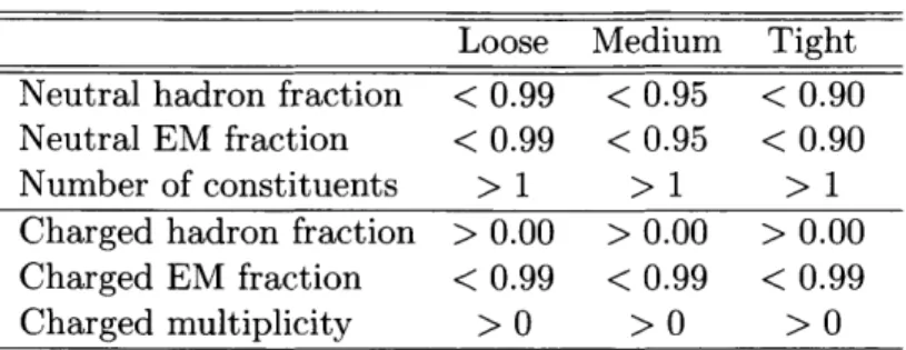
Loose Medium Tight Neutral hadron fraction < 0.99 < 0.95 < 0.90

Neutral EM fraction < 0.99 < 0.95 < 0.90

Number of constituents > 1 > 1 > 1

Charged hadron fraction > 0.00 > 0.00 > 0.00

Charged EM fraction < 0.99 < 0.99 < 0.99

Charged multiplicity > 0 > 0 > 0

Table 2.1: CMS jet quality criteria. We additionally enforce Jirl < 1.9.

in physics analyses [2].

Each event in the AOD format has a complete list of PFCs, which are particle-like objects containing the reconstructed four-momentum and a probable particle identification (PID) code. In addition, the AOD format has AK5 jets, which are clusters of PFCs identified by the anti-kt jet algorithm [33] with radius parameter R = 0.5. The AK5 jets come with jet energy correction (JEC) factors, including a correction for pileup using the area subtraction procedure [34]. They also have information needed to impose jet quality criteria (JQC), which are outlined in Table 2.1.

2.2

The MIT Open Data Framework

Because of the technical challenges involved in using CMSSW, we only use CMSSW to extract information from the AOD files, performing the actual physics analyses outside of the virtual machine environment. Building on the MOD software framework introduced in Ref. [19], we use a custom MODProducer module in CMSSW to translate each AOD file into a plain text MOD file. We then use a stand-alone C++ framework called MODAnalyzer to read in each MOD file and perform various jet analysis tasks using FASTJET 3.3.1 [35] and FASTJET CONTRIB 1.037 [36]. Finally, we convert the MOD files into compressed NUMPY data files (i.e. NPZ) such that we can use a variety

of PYTHON-based tools for analysis.

We made a number of improvements to MODProducer compared to Ref. [19]. In the previous version, the AOD files had to be downloaded ahead of time before converting to the MOD format. Now, AOD files are streamed online using the XRooTD [37] interface, which significantly reduces storage requirements. In the previous version, only valid LBs were converted to the MOD format. Now, all events are converted and the LB validation step is done within MODAnalyzer, which makes it easier to verify that the complete Jet primary dataset was processed correctly. We added additional physics information in the MOD format, including metadata about files, LBs,

18

and triggers. We added primary vertex information to implement CHS for pileup mitigation (see Chap. 3.2 below), made possible because the AOD files have a VertexCollect ion handle that can assign a charged-particle track to the closest collision vertex. We also added the ability to process

MC files provided by CMS in the AODSIM format, including both generation-level particles and

reconstructed PFCs.

For MODAnalyzer, the core class structure remains largely the same as in Ref. [19]. The main updates are for processing the MC files and for outputting intermediate text files for later conver-sion into the NPZ format. Since the bulk of our study uses PYTHON-based tools, the main role of MODAnalyzer is for initial jet selection and to access FASTJET information. Because of rare numerical rounding issues when converting from AOD to MOD, we recluster the PFCs into AK5 jets and compare against the CMS-provided AK5 objects, discarding any jets that do not have the same number of constituents or whose four-momenta disagree by more than 1MeV. As described in more detail in Chap. 2.5, we consider the hardest- and second-hardest jets for our analysis, after correcting the jet PT using the JEC factors and imposing the CMS-recommended "loose" JQC [38].

After the jet selection stage in MODAnalyzer, the rest of our workflow is in PYTHON, which helps speed up the overall development cycle compared to Ref. [19]. We used NuMPY [39] for data manipulation and MATPLOTLIB [40] to produce figures. In addition, we embedded our code in

JUPYTER notebooks [41] for enhanced transparency and portability. To assist future jet studies on

the CMS Open Data, our complete set of JUPYTER notebooks will be made available to the public, along with the corresponding jet datasets in NPZ form.

2.3

Triggers, Prescales, and Luminosities

The Jet primary dataset contains 30 triggers. We summarize these triggers in Table 2.2, indicating the number of valid LBs/events for which the trigger is present, as well as the number of valid events for which the trigger fired. These are single jet and dijet triggers, where the trigger names include the nominal PT requirement for the jet(s). For simplicity, we do not distinguish between trigger versions, denoted by suffixes like _v2, in our analysis. (The documentation for Ref. [1] claims that there are 5 LlFastJet trigger variants in the Jet primary dataset, but as far as we can tell, these triggers were introduced after Run 2011A was complete. These triggers are present in the corresponding simulated datasets, outlined in the next section.)

Trigger Name HLT-Jet30 HLT-Jet60 HLT-Jet8O HLT-Jet110 HLT-Jet150 HLT-Jet190 HLT-Jet240 * HLTJet300 HLT-Jet370 HLT-Jet800 HLT-DiJetAve30 HLT-DiJetAve60 HLT-DiJetAve80 HLT-DiJetAvellO HLT-DiJetAve150 HLT-DiJetAvel90 HLT-DiJetAve240 HLT-DiJetAve300 HLT-DiJetAve370 HLT-DiJetAve15U HLT-DiJetAve30U HLT-DiJetAve5OU HLT-DiJetAve70U HLTDiJetAve100U HLT-DiJetAve140U HLTDiJetAvel80U HLT-DiJetAve300U HLTJet240_Q 47,168 10,578,200 2,216,488 1,414,462.687 1.0 1.567 HLTJet270-0 47,168 10,578,200 1,280,355 1,414,462.687 1.0 0.905 HLTJet370_NoJetID 109,339 26,275,768 1,712,007 2,333,280.071 1.0 0.734 Total 109,428 26,275,768 26,275,768 2,333,286.137 Missing 89 6.066

Table 2.2: Q = "CentralJet30_BTagIP". Triggers in the CMS 2011A Jet primary dataset [1], restricted to LBs declared by CMS to be valid for physics analyses. Shown are the number of valid LBs/events for which the trigger is present and the number of valid events for which the trigger fired. Also provided are the effective luminosity tig _eff defined in Eq. (2.1), and the average prescale value (ptrig) and effective cross section a tr2g defined in Eq. (2.2). As discussed in Chap. A, there are 89 LBs in the CMS 2011A luminosity table [2] that are not represented in the Jet primary dataset, but they have a negligible impact on our analysis. The HLT-Jet300 trigger designated by a star is the one used for the jet studies in Chaps. 3 and 4.

20 LBs 109,339 109,339 102,447 109,339 102,447 109,339 109,339 98,555 109,339 47,168 98,555 98,555 91,663 98,555 91,663 98,555 98,555 98,555 98,555 10,784 10,784 10,784 10,784 10,784 10,784 10,784 10,784 Events 26,275,768 26,275,768 24,763,358 26,275,768 24,763,358 26,275,768 26,275,768 22,804,627 26,275,768 10,578,200 22,804,627 22,804,627 21,292,217 22,804,627 21,292,217 22,804,627 22,804,627 22,804,627 22,804,627 3,471,141 3,471,141 3,471,141 3,471,141 3,471,141 3,471,141 3,471,141 3,471,141 Fired 1,886,519 1,830,972 1,514,585 2,215,025 2,619,066 2,717,698 2,808,532 4,617,890 1,514,921 23,332 1,395,616 1,441,766 1,061,272 1,715,990 2,164,614 2,345,093 2,700,309 2,356,934 741,685 226,226 353,893 339,591 625,374 302,083 416,588 255,412 21,369 L trig [b eff [nb'] 12.567 293.986 901.352 6,172.430 33,521.114 114,843.687 392,659.479 2,284,792.618 2,333,280.071 1,414,462.687 20.585 539.491 1,474.722 10,583.561 59,292.115 208,109.103 800,844.351 2,284,792.618 2,284,792.618 1.841 45.628 298.084 2,061.075 4,314.114 25,144.074 48,487.453 48,487.453 (ptrig) 185,672.6 7,936.7 2,293.8 378.0 61.7 20.3 5.9 1.0 1.0 1.0 110,990.5 4,235.1 1,369.1 215.9 34.1 11.0 2.9 1.0 1.0 26,335.3 1,062.7 162.7 23.5 11.2 1.9 1.0 1.0 otrg [nb] 150,121.262 6,228.101 1,680.348 358.858 78.132 23.664 7.153 2.021 0.649 0.016 67,796.133 2,672.456 719.642 162.137 36.508 11.269 3.372 1.032 0.325 122,871.355 7,756.130 1,139.246 303.421 70.022 16.568 5.268 0.441

100 101 102 103 104 105

Cumulative Luminosity Blocks

106 106 104 102 100 CMS 2011 Open Data 0 2500 50000 75000 00000 1500 L ne 1 _Jet300_

0

Luminosity Block (time-ordered)

Figure 2-1: (a) Effective luminosity for the single-jet triggers as a function of the cumulative number of LBs, ordered in time. Note that the Jet300 trigger used for our jet studies turns on after around

50pb- 1 has already been collected, but this is a relatively small fraction of the total 2.3fb-- collected over the course of Run 2011A. (b) Effective cross section for the single-jet triggers in each LB. The flatness of these curves indicates that the trigger behavior is roughly constant around the entire run, apart from moments where the trigger criteria or prescale factors changed. The horizontal dashed lines correspond to the total effective cross section for that trigger from Table 2.2.

109

105

103

10'

OMS 2011 Open Data

Total CMS 2011 Open Data

Jet Primary Dataset

si- 1.Je Tr ersr

-Total Jet370 Jet300 Jet240 Jet190 Jet150 Jet110 Jet80 J et 6 0 0 -10-1 10-3 10-5

MrO-D)

0-LBs. Strangely, the luminosity information in Ref. [2] claims that there are 109,428 valid LBs in this run, leaving 89 LBs unaccounted for in the Jet primary dataset. These missing LBs only contribute 6nb 1 to the recorded integrated luminosity (compared to 2.3fb 1 for the whole 2011A run), so their absence has a negligible impact on our studies. We investigate the missing LBs in more detail in App. A 1.

Because the total data-taking rate at CMS is limited, the lower PT jet triggers are prescaled to only fire a fraction of the time they are active. The prescale factors satisfy ptrig > 1, with ptrg = 1 indicating an unprescaled trigger. (Strictly speaking, there is a separate prescale factor for the Level 1 (LI) trigger and the high-level trigger (HLT), but we always use pti9 to refer to

the product of these factors.) The trigger prescale factors are fixed within a LB but can change between LBs. The effective luminosity for a given trigger is:

trig =

Z

eff ti

bELBs Pb

where b labels a LB, Lb is the recorded integrated luminosity in that block, and pt7g is the associated

prescale factor. The effective luminosities for the Jet primary dataset triggers are reported in Table 2.2, along with their average prescale factors and effective cross sections:

t trig _Ntrig

(trig

trig eff - trig

eff eff

where "total=T

E-bb

the total number of events for which the trigger fired.

Our analysis is based on the substructure of individual jets, so we focus our attention on the

9 single-jet triggers in Table 2.2, omitting HLT_Jet800 since its events are fully covered by the

HLTJet300 trigger. Their effective luminosities as a function of the number of cumulative time-ordered LBs are plotted in Fig. 2.3. We see that as the integrated luminosity increases, some jet triggers have to be prescaled. We also see that the HLTJet300 trigger only starts acquiring data

partway through the 2011A run, coinciding with the HLT-Jet240 trigger being prescaled.

In Fig. 2.3, we plot the effective cross section in each time-ordered LB for the 9 single-jet triggers. The trigger behaviors are relatively stable over the course of the 2011A run, though there is a noticeable shift in the HLTJet80 trigger when its selection criteria changed. One can also see

'As this thesis was being finalized, we became aware of a subtle in the luminosity information. Our investigations are outlined in App. C. The subtleties do have only a negligible impact on the results presented here.

Table 2.3: Information about the MC event samples provided by CMS [3, 4, 5, 6, 7, 8, 9, 10, 11, 12,

13, 14, 15, 16, 17] from the PYTHIA 6 hard QCD scattering process. Shown are the generator-level

Pr ranges, the files used/available in each sample, the number of events used in our analysis, and the effective cross section oaC. Only the 8 MC samples with PT > 170 GeV are needed for the jet

studies in Chaps. 3 and 4.

when the HLT_Jet300 trigger turned on and when the HLTJet80 and HLT_Jet150 triggers were turned off.

Since HLT_Jet300 is the lowest PT single-jet trigger that is unprescaled (i.e. (ptrig) - 1), it

will be the sole trigger used in our substructure and jet topics studies (see further discussion in Chap. 2.5). For reference, the recorded luminosity for HLT_Jet300 as a function of time is plotted in Fig. B-1 of App. B.

2.4

Monte Carlo Event Samples

A key improvement in the CMS 2011 data release compared to 2010 is the inclusion of MC event

samples. For our analysis, we use samples of hard QCD scattering generated by PYTHIA 6.4.25 [42] with tune Z2 [43]. As summarized in Table 2.3, there are 15 exclusive samples with non-overlapping hard-scattering PT ranges [3, 4, 5, 6, 7, 8, 9, 10, 11, 12, 13, 14, 15, 16, 17], for a total of 13.4TB. They are labeled by CMS as QCDPt-MINtoMAXTuneZ2-7TeV-pythia6, where PT E [MIN, MAX] GeV. These events are then simulated and reconstructed using the CMS detector simulation [44]

lvi (> ~min PT 0 5 15 30 50 80 120 170 300 470 600 800 1000 1400 1800 Pn [GeV] -5 - 15 - 30 - 50 - 80 - 120 - 170 - 300 - 470 - 600 - 800 - 1000 - 1400 - 1800 -00 Total Files 55

/

/

/

/

/

/

/

/

/

/

/

/

based on GEANT4 [45].

Because of the steep dependence of the QCD dijet cross section on PT, the MC events have different weights, though the weights for all events in a single MC sample are the same. Therefore, when filling histograms, we have to rescale each MC event by the generated cross section

_~eff

divided by the number of events in the MC sample, as given in Table 2.3.

Both the generation-level and simulation-level objects are stored in AODSIM format by CMS, and we convert them to our MOD format using the MODAnalyzer software from Chap. 2.2. Because of the large overhead in processing the MC files, we only process the first 200 AODSIM files for each MC event sample, which gives us roughly half of the total MC events provided by CMS for the hard QCD process. Apart from the generation-level event record from PYTHIA, the AODSIM format is very similar to AOD. In particular, AODSIM includes reconstructed AK5 jets, simulated trigger information, as well as the addition of pileup. To save space, we only store the final-state particles in the PYTHIA event record, along with the 2 -+ 2 hard-scattering process for anticipated future studies related to parton flavor.

One subtlety in using the generation-level PYTHIA information is that there is a cutoff on the hadron lifetime above which they are considered stable. This cutoff is set to c T

stable = 10mm, which means that various hadrons with non-zero strangeness are considered stable, notably the

Ks meson. Typically, these strange hadrons decay within the CMS detector volume and are often

reconstructed as if the decay products came from the primary vertex. For example, Ko --+

ir-r-will typically be reconstructed as two pion-labeled PFCs. This leads to a mismatch in observables like track multiplicity unless we manually decay these strange hadrons. As a workaround, we load the generation-level event record into PYTHIA 8.235 and adjust the hadron lifetime threshold to

c rstable = 1000mm. Because the kinematics and flavors of the hadrons decay will not be the same as

in the CMS detector simulation, there is a slight mismatch when comparing a generation-level event to its simulation-level counterpart, though this issue does not arise when comparing histograms.

2.5

Jet and Trigger Selection

The jet studies in this paper are based on the two hardest PT jets in an event. This is motivated by the fact that 2 -- _{2 QCD dijet production at leading order yields two jets of equal PT. Therefore,}

considering the substructure of just the hardest PT jet (as in the studies of Refs. [20, 19]) is IRC (infrared and collinear) unsafe, since an infinitesimally soft emission can change the relative jet

108 . . .1 . . 108 [15, V

. ' '

CMS 2011 Open Data + Jet30 .CMS 2011 Simulation + + [15,30] GeV

Jet Primary Dataset Jet60 PYTHIA 6 Tune Z2 + + [30, 50] GeV

106 AK5 Jets, IrjetI < 1.9 J - 106 - AK5 Jets, ret I < 1.9 +

-++ Jet80 ₊ [50,85] GeV + + Jet110 0 [80,120] GeV + + Jet5O - 104 ++ [120,170] GeV i0~ ++ Jetl9O : e SJ++ [170,300 GeV 102 ++ Jet240 2 - [300,470] GeV Jet300 _{++ [470,600] GeV} 100 - Jet37O 100 - -+[600,800] GeV 0 200 400 600 800 0 200 400 600 800

Jet Transverse Momentum PT [GeV] Jet Transverse Momentum PT [GeV]

Figure 2-2: Raw PT spectrum for the two hardest jets in (a) the 9 single-jet triggers and (b) 9 of the

15 simulated MC samples, restricted to 1r et I < 1.9. These jet spectrum have JEC factors included

and JQC imposed. For the MC samples, the higher 6 datasets are shown in Fig. B-2.

ordering. On the other hand, considering more than two jets requires information beyond leading order, so we only consider the two hardest PT jets in our analysis.

The CMS single-jet triggers are designed to fire any time an event has a jet whose PT is above

a given threshold. Therefore, we consider the two hardest jets in an event as if they were inde-pendently selected by the triggers, correcting their PT values by the appropriate JEC factors. We impose the loose JQC, as outlined in Table 2.1. When we perform our substructure analysis, we require that the jets satisfy Ij4 et < 1.9 to make sure that the R = 0.5 jets are reconstructed fully

within the tracking volume that covers irtracker < 2.4.

In Fig. 2.5, we show the PT spectrum of the two hardest jets (i.e. two histogram entries per event) in the CMS 2011 Open Data, separated into the 9 single-jet triggers. We see that the triggers start to collect an appreciable number of jets when the jet PT matches the trigger name, asymptoting to a common smooth PT spectrum. In Fig. 2.5, we show the same PT spectrum in the CMS simulation, separated into the 15 MC samples. We see that the MC files have support mainly

in their designated PT ranges, albeit with a spread due to phenomena like initial state radiation (ISR) that change the overall event kinematics.

To simplify our physics studies, we use just one of the single-jet triggers. As mentioned above, we select HLTJet300 since this has the lowest PT threshold among the unprescaled single-jet triggers. Looking at Fig. 2.5, we can already estimate that HLT_Jet300 is fully efficient above PT > 375

1.2 .. 1.2

CMS 2011 Open Data CMS 2011 Simulation

AK5 Jets, 1,jet < 1.9 99 AK5 Jets, ,etI < 1.9 99(

1.11. 98%: 98%: 95%: - 95%: 901: :90%: -1 .0 --- -- -- --- -- -- --- -'-- 1 .0 - -- ---- --o 0.9 0.9 0 0.8 0.8 0.7 00.7

0.6 - ERF fit 0.6 - ERF fit

++ Jet300 ++ Jet300

0 - ' ' L ' ' '- 'L .

0 300 350 400 450 050 300 350 400 450

Jet Transverse Momentum pT [GeV] Jet Transverse Momentum PT [GeV]

Figure 2-3: Turn on behavior for the Jet300 trigger as a function of reconstructed jet PT. Arrows are drawn to mark the 375 GeV boundary where the trigger is essentially 100% efficient. (a) Relative efficiency in the CMS Open Data of the Jet300 trigger with respect to the Jet240 trigger.

(b) Absolute efficiency in the MC simulation of the Jet300 trigger. Both of these curves are fit to

an error function to determine the efficiency boundaries. From these, we conclude that the Jet300 trigger is fully efficient above PI > 375 GeV.

GeV, and we will quantify this statement below. Looking at Fig. 2.5, we see that all of the MC samples with PT > 170 GeV contribute appreciably to the PT > 375 GeV region, corresponding to

8 required MC event samples.

To determine where the HLTJet300 trigger is fully efficient, we compare its behavior to the HLTJet240 trigger. In Fig. 2.5, we consider events where the Jet300 trigger is present and the Jet240 trigger fired. We then plot the fraction of events where Jet300 fired as a function of jet

PT. Fitting the resulting fraction to an error function, we estimate that the Jet300 trigger is 99%

efficient (relative to Jet240) at 367 GeV, justifying our choice of PT > 375 GeV. For completeness, we plot these ratios for all of the adjacent trigger pairs in Fig. B-5 of App. B.

We can cross check our trigger efficiency study using the CMS simulated data. In Fig. 2.5, we plot the fraction of events where the simulated Jet300 trigger fired as a function of jet PT. Doing the same error function fit, we find that the simulated Jet300 trigger is 99% efficient (relative to an absolute scale) at 350 GeV, which is again consistent with our PT > 375 GeV choice. Since we are performing an exploratory jet study, we do not correct for this small trigger inefficiency in our analysis.

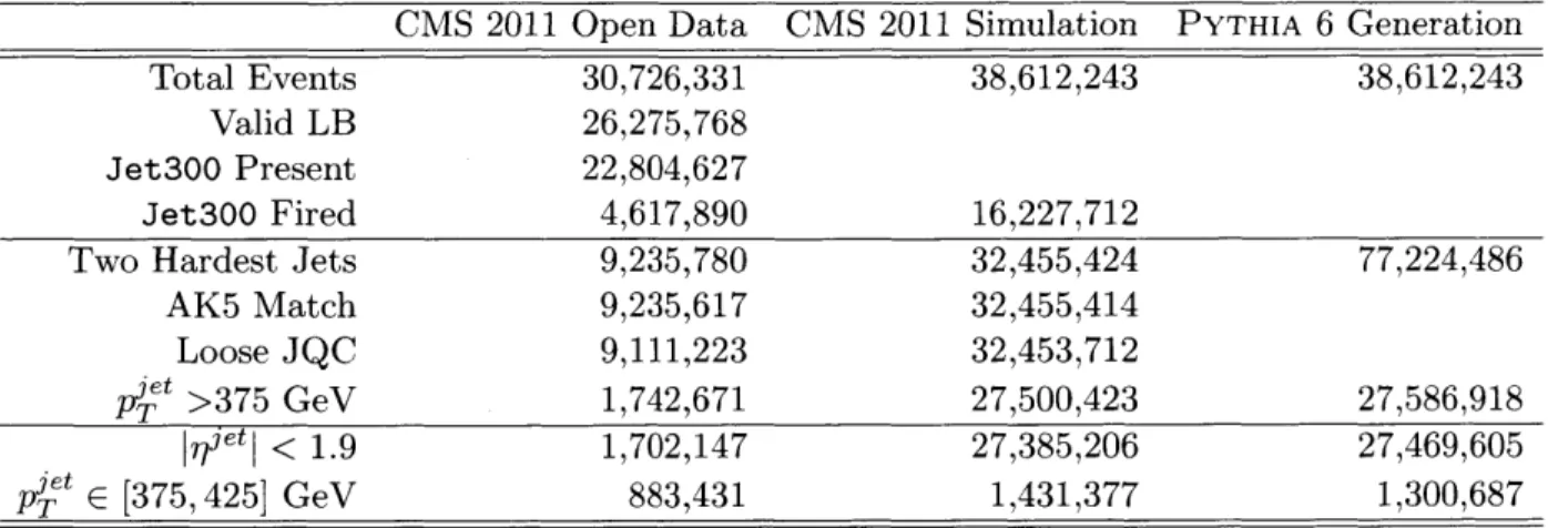
CMS 2011 Open Data CMS 2011 Simulation PYTHIA 6 Generation

Total Events 30,726,331 38,612,243 38,612,243

Valid LB 26,275,768

Jet300 Present 22,804,627

Jet300 Fired 4,617,890 16,227,712

Two Hardest Jets 9,235,780 32,455,424 77,224,486

AK5 Match 9,235,617 32,455,414

Loose JQC 9,111,223 32,453,712

et >375 GeV 1,742,671 27,500,423 27,586,918

1rdet I < 1.9 1,702,147 27,385,206 27,469,605

E [375,425] GeV 883,431 1,431,377 1,300,687

Table 2.4: Initial workflow and event selection for the jet studies in Chaps. 3 and 4. The first block ensures that the Jet300 trigger fired in a valid run, the second block ensures that the jets are high quality and the Jet300 trigger is fully efficient, and the third block imposes the baseline analysis criteria. Because our analysis is based on the two hardest jets, there is a factor of two increase between the first and second blocks.

Our initial workflow is summarized in Table 2.4. Because we consider the two hardest jets, there are twice as many jets in the analysis as the number of events. In order to have a more homogenous jet sample, we later impose the narrowerpJ;t E [375,425] GeV range for our substructure and topic

Chapter 3

Analyzing the Substructure of Jets

To validate the performance of the CMS detector for jet reconstruction, we present a variety of jet kinematics and jet substructure distributions derived from the CMS 2011 Open Data. There

are two main differences compared to a similar analysis performed in Ref. [19]. First, we can now compare the open data distributions to detector-simulated MC samples to check for robustness. Second, we have proper luminosity information [2] such that we can plot differential cross sections (instead of just normalized probability distributions).

3.1

Overall Jet Kinematics

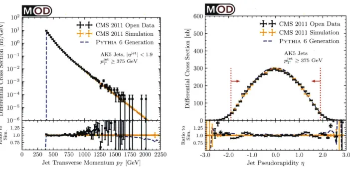
In Fig. 3.1, we show the PT spectrum of the two hardest jets, restricted to the region 1rjiel < 1.9

and p; t > 375 GeV. Here, we compare the CMS Open Data in black to the simulated MC samples in orange, finding very good agreement in the shape of the PT spectrum. Because PYTHIA is a leading-order generator, we have rescaled the MC events by an estimated NLO K-factor:

K = 1.15, (3.1)

where this value was chosen for R = 0.5 jets based off the material in Ref. [46]. We also show the generation-level PYTHIA distribution without detector simulation, which matches very well to the

CMS Open Data, indicating that the overall JEC factors have been chosen appropriately. Note

that these distributions only include statistical uncertainties, without any estimate of systematic uncertainties.

+C+ MS 2011 Open Data

+ CMS 2011 Simulation

-- PYTHIA 6 Generation

-CAK5 Jets, ,rietI < 1.9

ITlt > 375 GeV LU .L L-600 500 0 400 300 9 200 100 0 4 0 1.25 1.0 0.75 0 250 500 750 1000 1250 1500 1750 2000 2250

Jet Transverse Momentum PT [GeV]

I0J0OD)

-3.0 -2.0 -1.0 0.0 1.0 2.0 3.0

Jet Pseudorapidity 'r

Figure 3-1: (a) Jet transverse momentum spectrum, comparing the CMS Open Data to MC event samples at the simulation level and generation level. We consider up to two of the hardest PT

jets, restricted to

b7jetI

177et requirement removed. For both jet spectra, we see very good agreement between data and

simulation, indicating that we have properly processed the CMS Open Data, including appropriate

JEC factors. In these and all subsequent plots, the error bars indicate statistical uncertainties only,

with no attempt at estimating systematic uncertainties.

30 0 .0 E7 -C.8 0 102 101 100 10-1 10-2 10-3 10-4 10-5 10-6 1.25 1.0 0.75 + + CMS 2011 Open Data + + CMS 2011 Simulation PYTHIA 6 Generation AK5 Jets Pie 375 GeV P m

WA-CMS 2011 Open Data CMS 2011 Simulation

PID Candidate Total After CHS pT > 2 GeV Total After CHS pT > 2 GeV

11 Electron (e) 31,311 30,217 30,028 46,622 44,849 44,548 -11 Positron (e+) 31,506 30,438 30,263 45,704 44,007 43,702 13 Muon (ft-) 16,773 14,900 14,156 29,912 26,673 25,834 -13 Antimuon (p+) 17,462 15,323 14,556 30,894 27,400 26,540 211 Positive Hadron (7+) 10,747,712 8,167,309 5,645,324 19,026,243 14,017,136 9,605,247 -211 Negative Hadron (7r) 10,430,705 7,995,474 5,503,760 18,450,375 13,762,854 9,406,625 22 Photon (-y) 14,122,487 14,121,327 4,185,613 23,764,029 23,763,520 6,943,089 130 Neutral Hadron (KLj) 2,965,343 2,965,343 1,607,233 4,472,776 4,472,776 2,449,731

Table 3.1: Counts of PFCs by PID code, considering the constituents of the two hardest jets with the restriction IretI < 1.9 and 7T" E [375,425] GeV. The MC simulation has a larger number of

events than the CMS Open Data, and therefore more total PFCs. Note that the PID code is based on the PDG MC numbering scheme, but a code like 211 indicates any charged hadron candidate, not solely ir*

we find a small number of jets at larger pseudorapidities. Compared to the simulated data, the open data has more jets in the vicinity of Ir/jetl ~ 1.2 and fewer in the vicinity of Ir/Ieti ~ 0.0, indicating a possible issue with the pseudorapidity dependence of the JEC factors. That said, the overall agreement is very good, giving us confidence that we can make basic kinematic jet selections. For completeness, the jet azimuth spectrum is shown in Fig. B-4 of App. B, which exhibits the expected flat spectrum with small fluctuations due to detector inhomogenities.

3.2

Jet Constituents

In addition to the reconstructed AK5 jets, the CMS Open Data contains the complete list of PFCs, which allows us to calculate a wide range of jet substructure observables. Due to detector effects, though, one has to be careful in interpreting the PFC information. Ultimately, we will focus on track-based observables which have better reconstruction performance as well as better pileup stability.

In Table 3.1, we list the PID codes of the PFCs and their absolute counts in the jet sample with

lr/ejt < 1.9 and piet E [375,425] GeV, which is the jet selection we will use in Chap. 3.3 below.

Note that there are more events in the MC samples than the open data, so there is a corresponding increase in the number of total PFCs. The PID codes indicate the most likely particle candidate, using the PDG MC numbering scheme [47]. In particular, code 211 includes 7r+, K+, and protons

candidates, code 22 includes photon and merged 7r0 -- yy candidates, and code 130 includes K2

6000 2500

++ CMS 2011 Open Data + CMS 2011 Open Data 5000 CMS 2011 Simulation +2000

+

+

PYTHIA 6 Generation PYTHIA 6 Generation

4000AK5 Jets, et] < 1.9 AK5 Jets, 7-ietl < 1.9

A5Jet7't I 15009 E [375, 425] Giev 1500 et E [375,425] GeV \I CHS 3000 -% 1000 - 2000-1000 -- 500-1000 0 : :. 01 .t . .... 0 1.25 1 0 1.25 % 0 1.0 N - - - --1.0 C4 0.75 - 1 - 0.75 0 1 2 3 4 5 0 1 2 3 4 5

Neutral PFC Transverse Momentum PT [GeV] Charged PFC Transverse Momentum PT [GeV]

Figure 3-2: Transverse momentum spectra for (a) neutral PFCs and (b) charged PFCs, including

CHS to mitigate charged pileup. The CMS simulation captured the key features of the CMS Open

Data. Only for charged PFCs with p4FC > 2 GeV is there good agreement with the generation-level expectations from PYTHIA 6.

The counts in Table 3.1 include contamination from pileup. As shown in Fig. B-3 of App. B, there are typically - 5 pileup events per beam crossing. We have two ways to mitigate the effect of

pileup. First, inspired by the SoftKiller procedure [48], we impose a pTFC > 2 GeV cut on all PFCs, where this value is justified in Fig. 3.2. Second, we apply the CHS procedure to remove charged particles not associated with the primary vertex [49]. This is possible since MODProducer now stores vertex information (see Chap. 2.2 above), so we can remove charged jet constituents assigned to pileup vertices. (There are a small number of photon candidates that also have vertex information, which we assume are from converted photons.) Note that the CMS Open Data already includes a pileup correction for the jet pT via the JEC factors, but this is insufficient to correct substructure distributions. Though CHS cannot remove neutral particles from pileup, it does reduce the overall pileup contamination by a factor of - 2/3.

The PT spectrum of neutral PFCs is shown Fig. 3.2.a. The neutral PFCs do not benefit from

CHS, so there is a significant excess of neutral PFCs from pileup below around 2 GeV, compared to

generation-level expectations. That said, the CMS simulation appropriately captures this neutral pileup contamination. Because of finite calorimeter granularity, there is a depletion of moderate PT

neutral PFCs from merging. This merging results in an excess of higher PT neutral PFCs, which

can be seen in Fig. B of App. B.

The PT spectrum of charged PFCs is shown in Fig. 3.2.b. With CHS, the PFC PT spectrum is

rather similar between the CMS Open Data and the MC event samples, even at the generator level

and even going out to higher PT in Fig. B of App. B. The main difference is below 1 GeV, where one sees the impact of tracking inefficiencies. For this reason, we impose a cut of pTFC > 2 GeV for all of our jet substructure studies.

3.3

Jet Substructure Observables

In Fig. 3-3, we compare the CMS Open Data to the MC simulation for three classic substructure

distributions: jet mass, constituent multiplicity, and pg (transverse momentum dispersion)

[501.

Following the recommendations in Chap. 3.2, we always implement CHS and impose the pPFC >

2 GeV cut. In order to analyze jets with similar total PT, we focus on the relatively narrow range

of K t E [375,425] GeV.

For the left column of Fig. 3-3 using all PFCs, there is good agreement between data and

simulation. This suggests that PYTHIA 6 with tune Z2 has a reasonable model for jet fragmentation

and that the CMS simulation provides a faithful characterization of the detector response. That said, there are significant differences when comparing to the generation-level distributions, even after applying CHS for pileup mitigation. Roughly speaking, the CMS detector reconstructs fewer PFCs than expected, which is consistent with merging of neutral PFCs due to finite calorimeter

granularity. On the other hand, the CMS detector reconstructs a larger jet mass than expected, which is consistent with residual neutral pileup contamination.

For the right column of Fig. 3-3 using jet charged PFCs, the data, simulation-level, and generation-level distributions are much more similar. There is a small number of events in the open data with very low track multiplicity that are borderline for failing the JQC. While the CMS detector reconstructs fewer charged PFCs than expected from PYTHIA at the generation level, the difference is well within the theoretical uncertainties in MC generation (see further discussion in

Ref. [51]).

Since we will not be attempting to unfold the data, it is important to use observables that are robust to detector effects. For this reason, the focus of our topic studies will be on track-based observables.

0e 0 0 ~0 0 C 0 0 C 20 . ++ CMS 2011 Open Data + + CMS 2011 Simulation 15 -- PYTHIA 6 Generation

-q,, AK5 Jets, |₁itI < 1.9

p'T E [375,425] GeV 10 - ,, CHS, p Fc > 2 GeV 10 %.. 1. 0 20 40 60 80 100 12( Mass [GeV] 30 3 + CMS 2011 Open Data 25 + + CMS 2011 Simulation -- PYTHIA 6 Generation 20 _{AK5 Jets, ]} 7 1et|I < 1.9 pI * E [375,425] GeV 15 - -CHS, p FC > 2 GeV 10 5+ aMt01OpnDt 0 1.5 -1.25 _A[, 1.0-0.75 0.5 -0 20 40 60 80 Constituent Multiplicity 00 750 + CMS 2011 Open Data 75+ + CMIS 2011 Simulation 25 I 500 PYTHIA 6 Generation ?50 -AK5 Jets, lrdet

[

PR P t E [375, 425] GeV 00- CHS, pPFC > 2 GeV r50 - % -500 50 -. 0 O . .75 - -0 0 C 0 Cn C 0 0 2.0 20 .. + + CMS 2011 Open Data + + CMS 2011 Simulation 15 - . PYTHIA 6 Generation \ AK5 Jets, ,t|t I < 1.9 et E [375,425] GeV 10 - CHS, p FC > 2 GeV 0. .1 0 . II I . . 1.0Al - I .75 -0 20 40 60 8

Track Mass [GeV]

30 + CMS 2011 Open Data 25 + + CMS 2011 Simulation - - PYTHIA 6 Generation 20 _{AK5 Jets, ]} 27jtt < 1.9 p3e t E [375,425 GeV 15 CHS, pPFC > 2 GeV 0 -3 4 _1.5 .25

a

Transverse Momentum Dispersion

++ CMS 2011 Open Data

+ + CMS 2011 Simulation

PYTHIA 6 Generation

AK5 Jets, 17et|I < 1.9

I u-*~"%b 9,Pt E [375,425] GeV

:0 CHS, pPFC > 2 GeV

.5

jll *JUWI~ - -

-0.0 0.2 0.4 0.6 0.8 1.0

Track Transverse Momentum Dispersion

Figure 3-3: Classic jet substructure observables using (left column) all and (right column) charged PFCs. In all cases, we apply CHS and enforce pPFC > 2 GeV. The observables are (top row) jet mass, (middle row) constituent multiplicity, and (bottom row) transverse momentum dispersion

34 0 t 2 1 1t Qr 0 - WV OM - d 0

e*

-0

I

0

e*

-2.

-Chapter 4

A New Exploration of Jet

Classification

4.1

Review of Jet Topics Theory

We now consider the method of jet topics, a means of jet classification based on unsupervised machine learning first outlined in Refs. [52, 53, 54, 55] and adapted for use in jet physics by Ref. [28]. Topic modeling is a mechanism first proposed in the domain of computer science where a program takes in a corpus of documents on two topics (for example, law and biology) and returns a vocabulary for each topic. The algorithm provides a reliable means to separate out classical mixtures without any reference to the types or numbers of objects in these mixtures.

Surprisingly, this mechanism is quite effective at taking a mixture of quark and gluon jets (as is often produced at the LHC) and returning a set of characteristics for each type. Therefore, we may take two mixtures of jets, each containing different quark and gluon fractions, and return histograms of observables for pure "quark" or "gluon" categories. Table 4.1 lists the correspondence between the topics algorithm as applied to documents (in the original formulation) and to jets (in our formulation).

The efficacy of the topics algorithm is dependent on our dataset having three properties:

1. Sample independence, i.e. between our two mixtures of jets, the quark and gluon

charac-teristics do not depend on properties of the mixtures;

2. Different sample purity, i.e. our two mixtures of jets do not have the same quark or gluon fractions;

Topic Model Word Vocabulary Anchor word Topic Document Corpus Table 4.1: Main concepts used in the of quark and gluon jets.

Jet Distributions

Histogram bin Jet Observable(s)

Pure phase-space region (anchor bin) Type of jet (jet topic)

Histogram of jet observable(s) Collection of histograms

original topic modeling algorithm, as applied to our studies

3. Mutual irreducibility, i.e. the idea of a "quark" jet is not really the idea of a "gluon" jet

plus something different. We may use this condition to define what an anchor word is: an object that belongs exclusively to one of our two topics. For example, while the word "cell" may be used in both law and biology contexts, the word "mitochondria" is unambiguously a biology term. For our jet application, we will later define regions of phase space that can only be occupied by quark (or gluon) jets, called anchor bins.

Ref. [28] outlines the following key equations used to classify jet distributions, adapted from the original mixed models algorithm in Ref. [55]. If we consider a statistical mixture of jets made of quarks and gluons, we can write the composition as

p(x) = fqpq(x) + fgpg(x), (4.1)

where pq(x) and pg(x) are the quark and gluon jet distributions (respectively), fq and fg are the quark and gluon fractions, and x denotes a set of jet observables [28]. Note that for our jet analysis, we set

fg

f,

fq

fq)).

PMi (x) - K(MM₂)pM2(X)

pTI x) = 1

1 - ,x(M₁iM ₂)

(and similarly for pT2), where K is the reducibility factor given by

,-(Mil M2) = k ,

qf-2)'

(4.2)

(4.3)