Development of a two-dimensional model of blood microcirculation flows

Development of a Two-Dimensional Model of Blood

Microcirculation Flows

by

Kevin Sabo

Submitted to the Department of Aeronautics and Astronautics

in partial fulfillment of the requirements for the degree of

Master of Science in Aeronautics and Astronautics

at the

MASSACHUSETTS INSTITUTE OF TECHNOLOGY

June 2017

@

Massachusetts Institute of Technology 2017. All rights reserved.

Author

Signature redacted

Department of Aeronautics and Astronautics

May 25, 2017

Certified by...Signature

redacted...

al

Wesley L. Harris

C.S. Draper Professor of Aeronautics and Astronautics

Thesis Supervisor

Signature redacted

Accepted by .

...

Youssef Marzouk

Chairman, Department Committee on Graduate Theses

OF TECHNOLOGY co,

Development of a Two-Dimensional Model of Blood

Microcirculation Flows

by

Kevin Sabo

Submitted to the Department of Aeronautics and Astronautics on May 25, 2017, in partial fulfillment of the

requirements for the degree of

Master of Science in Aeronautics and Astronautics

Abstract

This thesis presents the development of a dimensionless blood microcirculation model for the study of blood microcirculation flows. It is a two dimensional, axi-ally symmetric, incompressible, Newtonian-flow, Krogh cylinder model subjected to axially periodic boundary conditions. This model formulation allows for the use of the streamfunction-vorticity formulation of the Navier-Stokes equation, which offers simplification to boundary conditions and also allows for the use of a non-uniform, collocated mesh. A streamfunction vorticity formulation of the Immersed Boundary Method is also developed, specifically for the boundary conditions along the immer-sed boundary (red blood cell membrane). Periodic boundary conditions are uimmer-sed, with the assumption of fully-developed flow, in order to focus on the effects of the transient diffusion of oxygen into the surrounding tissue, orthogonal to the capillary flow direction.

Thesis Supervisor: Wesley L. Harris

Acknowledgments

Grandma Sabo, this is for you. I know you said that I could be a doctor, but this is as close as I will ever get to blood.

I have many people whom I want to thank. If I forget anyone, I offer my sincerest apologies because so many have helped me get to where I am today.

First and foremost, thank you to Professor Wesley L. Harris. Professor Harris has given me a wonderful opportunity to work on a problem, one which I have never seen before, that offers a complete overview of the engineering process. Also, Professor Harris has also been an excellent source of wisdom in regards to general daily life as well. Having known him since I was a wee freshman here at MIT and having him advise me throughout my undergraduate and graduate careers, I can confidently say that I would not be here if it were not for his guidance and wisdom.

Next, I want to thank my parents, Steve and Sonya Sabo. They have watched me grow throughout the years and have always been an unwavering source of love and support. From sharing in my joy of getting into graduate school to taking a phone call at four in the morning because I was too stressed out to sleep, I cannot thank them enough.

I also want to thank all of my friends here at MIT who have helped me out in many ways. A special thanks goes to Eric Tu, the guy who has been there through pretty much all of MIT, and is even sitting here next to me as I write this statement

(he has no idea - Hi Eric!). To my friends who have been at my side throughout this

endeavor: Dominique Hoskin, Andrew Koff, Billy Moses, Alex Luh, Zachery Miranda, Andrew Zmolek, Louis Chen, Chris Gilmore, Jacquie Thomas, Tim Galligan, Haofeng Xu, Ben Couchman, Tony Tao, Theo Mouratidis, Jinwook Lee, Albert Gnat, Vince Wang, Derek Paxson, Georgi Subashki, Juju Wang, Maddie Jansson, Dolly Yuan,

Dakota Pierce

(7{(*#),

Finally, I want to thank the entirety of the faculty and staff here at MIT's Depart-ment of Aeronautics and Astronautics. Thank you Marie Stuppard and Beth Marois, both of whom keep all the deadlines in order and make it easy for us students to focus on courses and research. Thank you to Todd Billings and David Robertson, both of whom have given me countless hours of technical and life advice, as well as increased my repertoire of jokes and humor topics. Thank you Mark Drela for the laughs and for answering my endless stream of varied questions, despite being on sabbatical.

Contents

1 Introduction 15

1.1 Modeling Blood Microcirculation Flows . . . . 15

1.2 Sickle Cell Anemia: Example of The Importance of Understanding Blood Microcirculation Flows . . . . 17 1.3 Outline of Thesis . . . . 20

2 Previous Research and Motivation 23

2.1 Current Blood Microcirculation Models . . . . 23

2.1.1 Fluid Mechanics: Viscous Fluid Modeling of Microculation . . 24 2.1.2 Species Transport: Chemical Modeling of Oxygen Transport in

Capillaries and Surrounding Tissue . . . . 26

2.1.3 Membrane Mechanics: Cell Suspension Modeling of Red Blood

C ells . . . . 28

2.2 Motivation for Dimensionless Equations . . . . 30 2.3 Motivation: Thesis Hypothesis and Objectives . . . . 32

3 Development of Blood Microcirculation Model 33

3.1 Physical Model of Blood Microcirculation and Red Blood Cell System 33 3.2 Fluid Mechanics of the Microcirculation . . . . 36

3.2.1 Fluid Mechanics: Boundary Conditions . . . . 37

3.2.2 Benefits of Streamfunction-Vorticity Formulations . . . . 40

3.3 Oxygen Species Transport within the Microcirculation and Surroun-ding T issue . . . . 41

3.3.1 Oxygen Species Transport: Boundary Conditions . . . . 44

3.4 Red Blood Cell Membrane Mechanics and Interactions with the Mi-crocirculation . . . . 45

3.5 Governing Equations for Blood Microcirculation Model . . . . 47

3.5.1 Non-dimensionalization of Governing Equations . . . . 49

3.5.2 Non-dimensional Parameters . . . . 50

4 Implementation of Numerical Model 51 4.1 Immersed Boundary Method . . . . 51

4.2 Newton-Raphson Iteration Solver . . . . 53

4.3 Domain Discretization . . . . 54

4.4 Finite Difference Modeling of Non-Uniform Grids . . . . 56

4.4.1 Lagrange Basis Polynomials for Finite Differentiation . . . . . 57

4.5 Discretization of Governing Equations . . . . 58

4.5.1 Red Blood Cell Body Forces: . . . . 60

4.6 Boundary Conditions and Interface Points . . . . 64

4.6.1 Periodic Boundary Conditions Along Domain Inlet and Outlet 64 4.6.2 Flux Boundary Conditions Along Sub-Domain Interfaces . . . 64

4.6.3 Lagrangian Mesh: Membrane Boundary Conditions . . . . 67

4.7 Residual Formulations . . . . 70

4.7.1 Residual Formulation for Interior Points . . . . 70

4.7.2 Residual Formulation for Boundary Conditions . . . . 74

5 Concluding Remarks 81 5.1 Discussion of Results . . . . 81

5.1.1 Parametric Study of Blood Microcirculation Flows: A Non-dimensional Viewpoint . . . . 81

5.1.2 Immersed Boundary Method Using Streamfunction Vorticity Form ulation . . . . 82

5.2 IBM Coding Challenges . . . . 83

A Derivation of Equations of Motion - Fluid Mechanics 85

B Derivation of Equations of Motion - Oxygen Transport 91

C Derivation of Equations of Motion - Membrane Mechanics 101

D Non-Uniform Differentiation via Lagrange Basis Polynomials 109

List of Figures

1-1 (a) Data points collected, red dots representing presence of HbS gene and blue dots representing absence of HbS gene. (b) Raster map of

HbS gene frequency. (c) Historical map of malaria endemicity. Figure

and caption from Piel et al.' . . . . 18 1-2 Graphic depicting normal RBC versus sickled RBC behavior with key

difference being blockage of inlet to microcirculation passage. Image

courtesy of NIH (https:www.nhlbi.rih.gov"healthheaith-topics topics"scu). 19

2-1 Experimentally measured dimensionless pressure drop of human blood plasma (red circles) versus that of water (black dashed line), indicating non-linear, shear-thinning behavior (figure provided by Brust et al.[91). 26

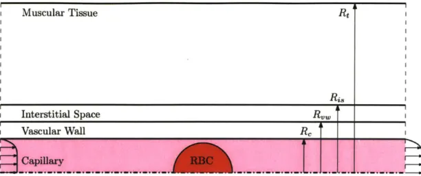
3-1 Visualization of the problem domain including the capillary, vascular wall, interstitial space, and muscular tissue sub-domains. . . . . 34

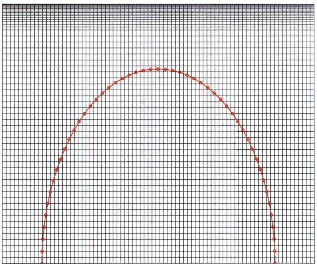
4-1 Non-uniform rectilinear grid for capillary sub-domain (unscaled). No-tice that the top capillary edge has a gradually denser mesh to account for the boundary layer formation. . . . . 55 4-2 Lagrangian mesh (shown in red with circles highlighting individual

mesh points) overlaying the Eulerian mesh (shown in black). . . . . . 56

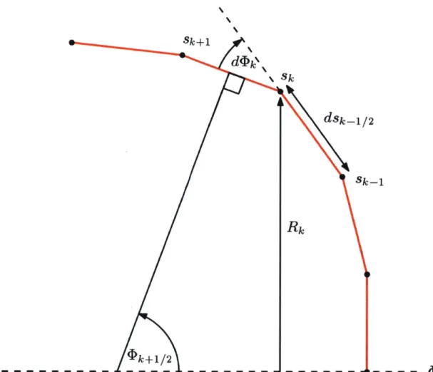
4-3 Red blood cell mesh geometry for calculation of constituent relations, visually defining all necessary variables. . . . . 61

B-1 Oxyhemoglobin curve as a function of partial pressure of oxygen. Image courtesy of www.anaesthesiauk.com. . . . . 95

C-1 Membrane tension, stress, and moments on a differential line element

of length ds. . . . . 102

List of Tables

3.1 Velocity and physical coefficients and parameters associated with se-parate sub-domains (from Vadapalli, Goldman, and Popel[ 7

]). .... 34

3.2 Additional model input values required for generation of governing equations for oxygen species transport. . . . . 35 3.3 Parameters required for the constituent relations of the red blood cell

membrane structural mechanics. . . . . 36

Chapter 1

Introduction

1.1

Modeling Blood Microcirculation Flows

The modeling of blood microcirculation flows is important for the study of nu-merous physiological processes, including the study of oxygen transport and other molecular transport to muscular tissues as well as various diseases, such as sickle cell disease. Results from such modeling and simulations can be used to help guide scien-tists, engineers, and medical professionals in creating new and effective treatment options for patients afflicted with various ailments and diseases.

There currently exists a large body of work on blood microcirculatory flows. As summarized by Gompper and Fedosov[ 1], two prominent observations have come from the study of these flows: the Fahraeus effect and the Fahraeus-Lindqvist effect. These effects lead to a seemingly reduced hematocrit in the capillary and an apparent vis-cosity reduction in the blood flow, respectively. Understanding these effects provides and understanding for the counter-intuitive results that they are responsible for.

The Fahraeus effect describes a seeming inconsistency regarding the hematocrit, the volume fraction of red blood cells (RBCs) in a blood vessel, in capillary flows. The overall hematocrit of the capillary flow is lower than that of the hematocrit observed at the capillary discharge. The underlying physics behind this effect resides with the RBCs occupying the center of the capillary flow, thus moving faster on average than the blood plasma which moves through the capillary.

The Fahraeus-Lindqvist effect describes the apparent viscosity reduction in the blood microcirculation flow as a function of the capillary diameter. This effect arises from the occupation of RBCs in the center of the capillaries, but in context with the RBC-free region near the capillary edges. This RBC-free region effects the apparent viscosity depending on the diameter of the capillary. The maximal reduction in viscosity is achieved in capillaries that are 7-8 pm in diameter. Below this diameter ranges results in RBCs producing increased blood plasma shear near the wall. Above this diameter range, the effect becomes negligible and the viscosity increases. This effect is quantified for the equivalent Hagen-Poiseuille flow viscosity, which can be expressed as follows[']:

7F

R4

Pap = -Ap- W (2.)

8 (Q + rR

_U)

Here, Ap is the pressure drop,

Q

These effects, along with numerous others, have been studied extensively in micro-circulation flows. While these effects provide key insight into the underlying physics, they do not provide a full description of all the effects occurring in these flows.

Instead of tackling specific effects, the aim of this research is to develop a fra-mework which tracks high-level, non-dimensional effects of various physical blood microcirculation properties. While some assumptions are made regarding the pro-perties of the microcirculation flow and surrounding tissue, the methodology behind the dimensionless formulation is general and can be applied to most systems. Instead of varying specific coefficients and running a plethora of experiments or simulations, varying dimensionless groupings of these coefficients can lead to more insight while decreasing experimentation and simulation time.

1.2

Sickle Cell Anemia: Example of The Importance

of Understanding Blood Microcirculation Flows

According to the National Institute of Health's Heart, Lung, and Blood Institute,

sickle cell disease is a genetic blood disorder in which the afflicted patient has

abnor-mal hemoglobin, hemoglobin S (HbS) or sickle hemoglobin, which causes the RBCs

to sickle upon their deoxygenation (source:

https://www.nhlbi.nih.gov/health/health-topics/topics/sca). It is an autosomal recessive disease, requiring a gene mutation

from both parents in order to be phenotypically active.

Sickle cell disease is found all over the world, but is largely concentrated in Africa

and some parts of Asia. The leading hypothesis for this occurrence is that the disease

offers resistance to malaria, a parasitic disease with mosquitoes acting as a primary

carrier. This hypothesis has been confirmed by Piel et all']. A geographical map

showing their Bayesian geostatistical analysis is shown in Figure 1-1. As can be seen,

the malaria holoendemic (defined as when essentially every individual in a population

is infected with a disease) and the frequency of the HbS gene go hand-in-hand.

Un-derstanding how to combat the negative effects of sickle cell anemia would directly

benefit a large population.

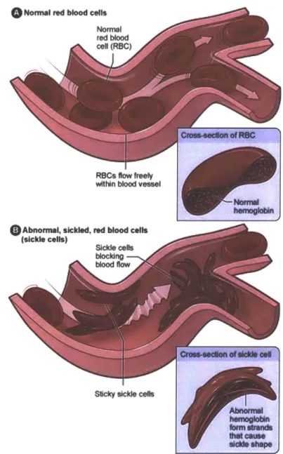
The phenotypical signature that sickle cell disease is commonly known for is the

formation of RBCs with a sickled shape, as can be seen in Figure 1-2. When an RBC

releases oxygen (oxygen unbinds from the hemoglobin protein), the RBC retains its

normal shape in a healthy patient. However, in afflicted patients, the RBC sickles,

which can lead to capillary vessel occlusion, a condition when the capillary becomes

clogged. When this event happens, the tissue downstream of the blockage receives

little to no oxygen, leading to painful events called crises.

An understanding of the transient conditions which lead to RBCs sickling can

potentially be found from a blood microcirculation model. In particular, a

dimen-sionless model can isolate which physical effects dominate the transient state from

normal RBC behavior to sickled RBC behavior. While the sickled RBC model

requi-res some extra steps[

_{a dimensionless microcirculation model framework will help}

HbGdIP.It Me po

4

b

Figure 1-1: (a) Data points collected, red dots representing presence of HbS gene and

blue dots representing absence of HbS gene. (b) Raster map of HbS gene frequency.

o

COOSS-890110 of FtSC

witin blood ve"s

hermogkkin

Abnoma, sickled, red blood cells

(sickle cells)

Sickle cobs

blocing blood flow

- Crows-edon of old* all

S~cky sickle cells

AbnonnyM

I*a cause dieM* shap

Figure 1-2: Graphic depicting normal RBC versus sickled RBC behavior with key

difference being blockage of inlet to microcirculation passage. Image courtesy of NIH

to uncover trends which govern RBC sickling.

1.3

Outline of Thesis

This thesis is composed of five chapters.

Chapter 1:

The first chapter covers the general importance of modeling blood flows,

speci-fically that of blood microcirculation flows. An example for context is given in the

study of sickle-cell anemia.

Chapter 2:

The second chapter provides an overview of previous research and motivation

for the continual study of research problems in this field. It will first review the

background work done on blood microcirculation models, covering the fluid

mecha-nics, oxygen transport, and membrane mechanics. Next, the importance of

non-dimensionalization is discussed in the context of canonical fluid mechanics problems

and how those techniques may be applied to hemodynamics problems.

Chapter 3:

The third chapter develops the physical model used in this work for the blood

microcirculation problem. The domain and sub-domains are established and the

assumptions pertaining to the problem domain and sub-domains are laid out. The

fluid mechanics of the blood plasma and cellular cytoplasm are explored in depth

with the appropriate modeling assumptions stated. The oxygen transport equations

are also developed for the various sub-domains. The cellular membrane mechanics

are developed from first principles and the resulting constituent relations are found

with the appropriate modeling assumptions. Lastly, the resulting system of equations

are non-dimensionalized in order to obtain the non-dimensional parameters that are

of interest to hemodynamicists.

Chapter 4:

The fourth chapter covers the simulation algorithm and code implementation. The Newton-Raphson Method (or Newton Method) for root-finding is discussed. How this method is applied to finite difference code is also covered. Non-uniform mesh techni-ques are developed for the problem in order to mitigate numerical boundary layer issues. The resulting domain discretization (meshing) is then discussed, paying spe-cial attention to unique requirements for the Immersed Boundary Technique. Finally, the discretization of the governing equations is reviewed and the appropriate boun-dary conditions discussed for the domain, sub-domains, and cellular membrane.

Chapter 5:

The fifth chapter of this thesis is dedicated to the discussing of the results of the research. Comparisons to previous work are made and recommendations for future work are presented. The key focuses for future work involve the extended use of the non-dimensional framework developed as well as potentially better techniques for simulating the problem, such as a finite element method with adaptive grid generation.

Chapter 2

Previous Research and Motivation

2.1

Current Blood Microcirculation Models

This chapter presents the high-level thoughts and modeling assumptions of some previous blood microcirculation models. There is a large body of literature regarding blood microcirculation modeling techniques, and a summary of this body may be found in Gompper and Fedosov 1. This chapter provides the essential motivation for the modeling done in this thesis work.

The model problem is the Krogh cylinder model, developed by August Krogh in 1919. It first started out as a 3-layer model, consisting of a red blood cell, a capillary containing blood plasma, and muscular tissue. Its intended use was to model the effects of oxygen diffusion through a cylindrical capillary tube, and has done so successfully for nearly 100 years. Vadapalli, Goldman, and Popell7 and Le Floch-Yin['] have used a more advanced 5-layer model, adding a vascular wall layer and an interstitial space layer in between the capillary and muscular tissue layers. Also, the red blood cell contains the oxygen-fixing protein, hemoglobin, and the muscular tissue includes the oxygen-fixing protein, myoglobin, both layers having their own set of governing equations.

2.1.1

Fluid Mechanics: Viscous Fluid Modeling of

Microcula-tion

Blood microcirculation flows occur in narrow capillaries ranging from 2 Pm to

10 pm in diameter. The flow is not homogeneous due to the fact that red blood cells

exist inside the blood plasma, leading to a coupled interaction between the red blood cells and the blood plasma.

Blood plasma is approximately 92% water.[ 9] Previous models [2][8][131 have assu-med that the blood plasma in the microcirculation is an incompressible, Newtonian, viscous fluid that can be modeled by the relevant Navier-Stokes equations. Most recent works also make this assumption, as stated by Sousa et al. [14] However, it has been experimentally demonstrated with sufficient confidence that blood is a complex, shear-thinning fluid (refer to Figure 2-1), leading the authors to strongly recommend the modeling community to incorporate the shear-thinning effects into new models.[ 9] The red blood cells are assumed to be fluid-filled "sacks" that contain cellular cytoplasm and hemoglobin proteins.[2 ] The fluid properties of the cell are assumed to be similar to that of the blood plasma (e.g. incompressible, Newtonian, viscous fluid) surrounding the cell, with a few minor differences (e.g. density and dynamic viscosity). From a dimensionless perspective, the Reynolds number of the blood plasma and cellular cytoplasm, relative to the capillary diameter, are different.

Since these fluids have different Reynolds number, it is reasonable to expect that the red blood cell membrane mechanics will be affected by this change. In previous work,[2_{] the density was chosen to remain constant between the blood plasma and}

cellular cytoplasm while only varying the dynamic viscosity. The blood plasma and cellular cytoplasm density was taken as 1025 kg/m3, despite the latter being reported to be slightly larger at 1125 kg/m3. In the Newtonian fluid assumption, the affect on the Reynolds number due to this difference would be negligible, [2] but this affect is not negligible in the copmlex, shear-thinning fluid assumption.

In the context of the current research that this thesis presents, the fluid will be assumed incompressible, Newtonian, and viscous for simplicity in deriving and

imple-menting a new non-dimensional model using a streamfunction-vorticity formulation of the fluid transport equations. It is strongly recommended that viscoelasticity ef-fects be considered in future research, as Reynolds number of blood microcirculation flows are 0(1), with Figure 2-1['] showing the sensitivity to Reynolds number at these lower values.

Limitations of Newtonian Fluid Assumption

The blood microcirculation flow in this work is assumed to be Newtonian in nature, or for the isothermal, incompressible assumption, that the viscosity coefficient /L is

constant. However, it is observed in reality that blood is a complex fluid due to the

suspension of blood cells, proteins, mineral ions, hormones, and glucose.[

]

The work done by Brust et al.

] show that blood plasma is a shear-thinning

complex fluid (i.e. the viscosity decreases under increased strain rate). Brust et al.

experimentally showed, via the use of a microfluidic contraction-expansion device, the dimensionless pressure drop as a function of the Reynolds number for human blood plasma versus that of water (see Figure 2-1).

Figure 2-1 clearly indicates a non-linear, shear-thinning behavior of human blood plasma as the Reynolds number increases. However, water exhibits no change in dimensionless pressure drop as the Reynolds number increases over the indicated range.

In the upper-right corner of Figure 2-1, the actual pressure drop is measured

against the volume flow rate. Water (black) exhibits a linear relationship while the

human blood plasma (red) deviates slightly in the intermediate flow rate range of

100-600 micro-liters.

Brust et al. conclude that the viscoelastic behavior (shear-thinning) of human

blood plasma is significant and recommend that it should not be ignored in future

blood flow modeling. They also indicate that the viscoelasticity may lead to

vis-coelastic flow instabilities, especially when RBCs are present at values around 50%

1.

25 0

s

1.4-

0

0' 8 40'66 6 1000

16E _ _{ow Rate (.AfnIn)}

-

1.2

-o Plasmia

a)

0E

1.

10

_{150. 20}

₂₅₀

₃₀₀

Re

Figure 2-1: Experimentally measured dimensionless pressure drop of human blood plasma (red circles) versus that of water (black dashed line), indicating non-linear, shear-thinning behavior (figure provided by Brust et al.[1]).

2.1.2

Species Transport: Chemical Modeling of Oxygen

Trans-port in Capillaries and Surrounding Tissue

As stated previously, the Krogh cylinder model was developed for the study of oxygen flow in blood microcirculation flows. The original 3-layer model has developed into an advanced 5-layer model[ 2][13] which has proven versatile in its development

over the past nearly 100 years.

The model used by Secomb et al and Le Floch-Yin consists of a simple cylindrical geometry that is layered similar to that of a cake (see Figure 3-1). The innermost layer is the capillary domain which includes the blood plasma and the red blood cell layer. The capillary is surrounded by the vascular wall, the vascular wall is then surrounded

by the interstitial space, and the interstitial space is surrounded by the muscular

tissue, thus yielding 5 layers. The red blood cell layer contains hemoglobin proteins which can bind with oxygen and the muscular tissue layer consists of myoglobin proteins which can also bind with oxygen.

In order to model the oxygen concentration dynamics, advecting-diffusion trans-port equations were developed in the form

Oc(21

-- + (- V) c = DV2 _{c+R (2.1)}

at V

where c represents a scalar quantity (in this case, the concentration of oxygen). Upon invoking Henry's law

2 = (2.2)

P0₂

where ao2 is the oxygen solubility coefficient and po2 is the oxygen partial pressure.

This statement leads to the governing equations for oxygen taking the form

O0

o

_R

_(2.3)

2 + (W. V)Po₂ = - P02 +

-The first term represents unsteady effects, the second advective effects, the third diffusive effects, and the fourth reaction rate chemistry with the oxygen-fixing protein effects.

A similar transport equation is developed for the saturation of the oxygen-fixing

proteins, which is coupled to the oxygen partial pressure equations via the reaction rate term.

as+ (- V) S = DV2S - R' _(2.4)

Through the reaction rate terms R and R' (which are not equivalent in this repre-sentation), the equations are coupled and the effects of the binding and unbinding of oxygen to the proteins is adequately captured.

The detailed derivation and explanation of these equations can be seen in Chapter

2.1.3

Membrane Mechanics: Cell Suspension Modeling of Red

Blood Cells

In the previous work of Le Floch-Yin, the red blood cell membrane was assumed to be an axisymmetric, deformable shell. The shell undergoes deformations in time due to the fluid interactions of the blood plasma and cellular cytoplasm with the membrane. These interactions are captured via a body force model, represented as

f,

full derivation, see Appendix A):

= Vp +vV2_{'U+ -f (2.5)}

Dt p

However, how the body forces are calculated depends on the mechanics of the red blood cell membrane. For these mechanics, constituent relations are derived.

The first constituent relations for the red blood cell membrane deformations are developed in Evans and Skalak's Mechanics and Thermodynamics of

Biomembra-nes:[ 5 dA t= o+ K - (2.6) dAo td (A2-A2 (2.7)

2 1

where t is the isotropic mean tension, td is the shear deviatoric term, and m is the

bending moment about a membrane point in any principal direction. Here, o-, is the

membrane's reference state isotropic tension, K is the isothermal area compressibility

modulus, K is the 2-D shear modulus, B is the isotropic bending modulus, dA is the dAO

area change with respect to the reference state, A, and A2 are extension ratios in the

reference directions such that dA = AI 1, k is the total local curvature, and ko is the reference local curvature.

While this model proves to be successful, some modifications to better capture the interaction between bending and tension forces were carried out by Secomb in

1988.12 Secomb added the assumption of axisymmetry to the model and removed

terms related to area changes that were not of leading order. The new constituent relations used are:

t _{o-o + K}

(2.9)

2 dAO

ta-to 1 1

td - t - - - K(A2 - A -2_{) B (ks - ko) (ks + ko - ko) (2.10)}

2 2 2

m = B (ks + ko + ko) (2.11)

where s and 0 are curvilinear coordinates following the membrane surface.

Equilibrium equations were derived in order to incorporate the constituent relati-ons into the body force model:

AP = -1tks - tko Rq) (2.12) R ds 1 d(Rts) 1 dR _(2.13) -Rds _{R ds} - t _{R ds}_ - qsk₅ 2.3 dm 0= d + qs (2.14) ds

where Ap is the local pressure difference between the external and internal fluids (local normal force per unit area), r is the local shear stress in the s direction (local tangential force per unit area), and the equation (2.14) represents the local moment per unit area, which equals zero in this instance as the red blood cell is suspended in fluid (thus unanchored, so no external moments apply). The new terms introduced are R, which pertains to the local membrane radius and is a function of s, and q., is the shear force per unit length in the membrane and is also a function of s. For a

complete derivation, see Appendix C.

For future research, it is recommended to use a viscoelastic model which captures the behavior of the red blood cell membrane with non-negligible viscoelastic effects. Work done by Tzeren et all15] [161 develop constitutive relations that model the effects from the viscoelastic behavior. The viscoelastic modification to equations (2.9)

-(2.11) is only seen in equation (2.10), and is shown below:

1 A) 1 __ (2.15

td=

(A

A

B (ks -

+

-

A(2.15)

2 s 5 2 (As Ot

where the viscoelasticity is a time-dependent behavior.

2.2

Motivation for Dimensionless Equations

Studying problems from a dimensionless viewpoint offer advantages for both the formulation of the problem and the insight gleaned from the results of the problem. These benefits can be explained in three parts. For a highly detailed explanation, please refer to B. Zohuri's textbook on dimensional analysis. [101

1. Reduction of Variable Count

First, finding dimensionless parameters may reduce the number of variables in the problem. Taking the Reynolds number as a common example of fluid mechanics, one can see that it is made of up four variables. If we were to look for the solution of some function, the functional form would be as follows:

F = f (U, L, p, p) (2.16)

However, upon non-dimensionalizing the function in equation (2.16), the Reynolds number is formed:

F f(Re = pUL (2.17)

variables from four to one, a dimensionless curve can be formed. If a high fidelity

mapping of the function

f

are required. By reducing the variables non-dimensionally to one, now only 100

experiments are required.

2. Insight into Governing Equations

The second benefit is that pertaining to the models developed for a particular governing equation or set of governing equations. As seen in Appendices A, B, and

C, the governing equations naturally form dimensionless parameters. This formation

of dimensionless parameters reveals key insights into the governing physics of the problem.

For instance, the Reynolds number describes (non-dimensionally) the ratio of ad-vective forces to frictional forces. By adjusting this parameter, one may characterize how much advection and diffusion occur in the fluid.

3. Similitude

The third benefit pertains to that of similitude. Similitude has three requirements: geometric similarity, kinematic similarity, and dynamic similarity.

Take an airfoil as an example. In order to test its flight characteristics, it may be cumbersome or infeasible to test a full-scale model. Engineers instead will test a scale model, preserving the shape of the airfoil, but shrinking it to an appropriate and manageable size for testing.

However, preserving the shape (enforcing geometric similarity) is only one requi-rement. The second requirement is kinematic similarity. Formally, the fluid over the airfoil in both the full-scale and scaled test cases must undergo similar time rates of change or change of motions. In other words, quantities related to motions or how things move must be similar.

The final similarity requirement is that of dynamic similarity. This requirement pertains to the ratio of forces acting on the system. In the case of the airfoil, the Reynolds number is a key measure of the ratio of inertial (advective) forces to viscous

(frictional) forces. If the full-scale and scaled cases are ran at the same Reynolds number, they are said to have dynamic similarity.

If these three criteria are met, a problem is said to have similitude. The non-dimensional solution to the model that governs a particular problem can then be rescaled to the required dimensions. Doing this for blood microcirculation flows al-lows for the scaling of physics pertaining to blood plasma viscosity, oxygen diffusion throughout the capillary to the muscular tissue, study the effects of variable hemo-globin and myohemo-globin concentration, as well as other mechanical and chemical effects.

2.3

Motivation: Thesis Hypothesis and Objectives

The first goal of this thesis work is to provide a dimensionless perspective to blood microcirculation flows in order to reduce the number of necessary simulations required to gain valuable insight into the problem and to take advantage of similitude. With these three principles evoked in the presented model, the results from a database of parametric studies (future work) should be able to guide medical professionals in developing new drugs and new therapeutic treatments that directly affect sickle cell crises.

The second goal of this thesis work is to generate a user-friendly simulation using the Immersed Boundary Method (IBM) technique. While the IBM is conceptually intuitive to understand, it presents unique challenges in the approximation of a mo-ving boundary and its boundary conditions on the flow fields inside and outside of the moving boundary. In the context of the red blood cell membrane, a zero-velocity boundary condition and a normal oxygen mass flux boundary condition must be satis-fied on and across the membrane, respectively. Enforcing these boundary conditions is a challenging task and leads to some undesirable arbitrariness in their implemen-tation. The new goal is to understand why the arbitrariness arises and to provide a clear path forward in the discretization of this problem.

Chapter 3

Development of Blood

Microcirculation Model

This chapter presents the blood microcirculation model. First, an overview of the model is presented, including key assumptions and model geometry. Next, the details of the model are presented, including the fluid dynamics of the blood microcircula-tion environment, oxygen species transport, and red blood cell membrane mechanics. Finally, the governing equations are summarized and non-dimensionalized.

3.1

Physical Model of Blood Microcirculation and

Red Blood Cell System

The model used in this thesis is a modified approach to the work done by Le

Floch-Yin.[2] It consists of a two-dimensional, axially-periodic domain made up of

five sub-domains: the red blood cell, the capillary, the vascular tissue, the interstitial space, and the surrounding muscle tissue. A visualization of this can be seen in Figure 3-1.

It is assumed to be symmetric about the centerline of the capillary, neglecting any variations in capillary flow area (and effects associated with vary vessel size) along the main axis of the capillary. This assumption ensures symmetry across the capillary while simultaneously reducing code complexity and runtime.

Muscular Tissue RI

Interstitial Space R

I Vascular Wall Rc

Figure 3-1: Visualization of the problem domain including the capillary, vascular wall, interstitial space, and muscular tissue sub-domains.

Each sub-domain has its own set of physical coefficients and parameters. While some of the coefficients are equivalent, this fact is not generally the case. These values are listed in Table 3.1 (the data are taken from work done by Vadapalli, Goldman,

and Popell7 1).

aM

V V Dos 2 m/3 [Hb] [Mb] M

(m/s) (M2/s) (M2 /s) (mol/m OIM) (MOI/M3) (MOl/M3/s)

Cytopam (v, vy) 5.2356 -10-6 9.47 -10-10 1.3118. 10-3 21.099 0 0 Plasm (V vy) 1.3659. 10-6 2.40 10-9 1.0906 10-3 0 0 0 Vascular 0 - 8.73 -10-10 1.5097. 10-3 0 0 3.8811 .10-3 Wall ____ Interstitial 0 - _{2.18 -10-9 1.0906. 10-3 0 0} 0 Space Tissue 0 - 2.41-10-9 1.5059. 10-3 0 0.4 6.1321 .10-3

Table 3.1: Velocity and physical coefficients and parameters associated with separate sub-domains (from Vadapalli, Goldman, and Popel[71).

The velocity vector V' only exists in the RBC cytoplasm and the blood plasma as those two sub-domains are the only sub-domains with bulk fluid motion. Thus, the kinematic viscosity v (= p/p) only takes on a value in those two sub-domains. D

represents the diffusion coefficient for oxygen, a the oxygen solubility constant, [Hb] and [Mb] the molar concentration of hemoglobin and myoglobin , and M a

hypot-hesized oxygen consumption rate constant. Not that in some of the sub-domains, the molar concentration of hemoglobin and myoglobin go to zero, thus eliminating the associated reaction rate effects in those regions. Also note that the vascular wall and muscular tissue are the only sub-domains hypothesized in previous work[ 2 _to

consume free oxygen.

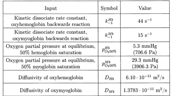
These coefficients and parameters arise in the governing equations presented in the model. However, for the formation of the oxygen transport equations, these pa-rameters do not make up the complete set of required model inputs. The complete derivation of these equations can be seen in Appendix B. The additional inputs re-quired are listed in Table 3.2. Table 3.1 and Table 3.1 complete the list of rere-quired input parameters for the model continuum model.

Input Symbol Value

Kinetic dissociate rate constant, k Hb 44 -1

oxyhemoglobin backwards reaction -1

Kinetic dissociate rate constant, _{kMb 15 s-1} oxymyoglobin backwards reaction -1

Oxygen partial pressure at equilibrium, Hb 5.3 mmHg

50% hemoglobin saturation P0_{2 5 0}% (706.6 Pa)

Oxygen partial pressure at equilibrium, Mb 29.3 mmHg

50% myoglobin saturation P0250% (3906.3 Pa)

Diffusivity of oxyhemoglobin DHb 6.10- 10-11 m2_/s

Diffusivity of oxymyoglobin DMb 1.3783 -10-11 m2

/s

Table 3.2: Additional model input values required for generation of governing equa-tions for oxygen species transport.

The last set of parameters needed are those for the structural mechanics and associated constituent relations of the RBC membrane. These parameters are listed

in Table 3.3.

The initial isotropic tension in the RBC membrane's resting, unstressed state is represented as -o. The isothermal area compressibility modulus K, often referred to as the 2-D bulk modulus, measures the membrane's resistance to surface area changes.

Input Symbol Value

Initial isotropic tension in membrane 01- 7- 10-2 kg/s2 Isothermal area compressibility modulus K 0.5 kg/s2

Membrane bending modulus B 1.8. 10-19 kg m2

/s2

Membrane shear modulus K 4.2 _ 10-6 kg/s2

Table 3.3: Parameters required for the constituent relations of the red blood cell membrane structural mechanics.

The bending modulus B quantifies the membrane's resistance to bending. Finally, the membrane's shear modulus r. represents the membrane's resistance to shear stresses acting on the membrane. These values used are in accordance with the work of Evans

and Skalak5'] and Halpern and Secombl81.

3.2

Fluid Mechanics of the Microcirculation

The blood plasma and red blood cell cytoplasm are assumed to be incompressible, Newtonian viscous fluids. This assumption allows for the use of the incompressible forms of mass continuity and the Navier-Stokes equations to be used as the fluid equations of motion, with associated body force

f:

V

0

Dii 1

1-Dt=---Vp+uv2+ -f

Dt p p (3.2)

Given that the model is assumed to be fully two dimensional, the problem can be simplified to a streamfunction vorticity formulation:

OW

_23.1

~+(6

at

pV

f

This formulation has the advantage of reducing a three variable vector transport system of equations to a two variable scalar transport system. The approach allows for a reduced computation time due to the reduced number of independent variables as well as a simpler use of a collocated mesh, as opposed to a staggered mesh, to compute on. While a collocated mesh can be used for the traditional representation of the Navier-Stokes equations, it is often difficult to run (refer to section 3.2.2). Bueno and Harris [3] also used this formulation for the blood plasma fluid dynamics, but did so on a staggered mesh and also left the formulation in its dimensional form. In order to better characterize the solutions to these governing equations and isolate the dynamics of the problem, the nondimensional form of equations (3.3) and (3.4) are used:

w* + v*2* =

o

+ (z* V*) w* = V2W* + V* x f* (3.6)

at* Re

From the nondimensionalization, the Reynolds number Re is found as a key nondi-mensional parameter of interest. The Reynolds number measures the ratio of inertial (advective) forces to viscous (diffusive) forces and can be used to isolate the mecha-nics of the problem. For instance, in high Reynolds number flows, viscous forces are small such that momentum diffusion is largely contained primarily in small viscous layers along solid surfaces (known as boundary layers).

For a more detailed derivation of this model, refer to Appendix A. For a more in-depth discussion of the Reynolds number, refer to Section ??.

3.2.1

Fluid Mechanics: Boundary Conditions

The boundary conditions for the fluid mechanics of the blood plasma are similar to that of pipe flows.

First, along the outer edge of the capillary sub-domain, a solid wall zero-velocity (no-slip and no-flux) boundary condition is applied. This boundary condition corre-sponds to a constraint on the first-derivative of the streamfunction at the capillary wall, namely the first-derivatives in both the x-direction and y-direction are equal to

0:

U wa -

-0

19y

- =0 (3.8)

In the streamfunction vorticity formulation, these are enforced via setting the wall to be a streamline (i.e. T is equal to a constant) and substituting equations (3.7) and

(3.8) into equation (3.5). Doing so results in the following set of residual equations:

R1j wall - c = 0 (3.9)

2 a *+ 2 =0 (3.10)

where c is a constant, which equals the non-dimensional capillary radius length in order to satisfy the non-dimensional volume flow rate of the blood plasma through the capillary.

The boundary condition for the centerline is a symmetric boundary condition. Physically, this corresponds to a streamline with zero vorticity. Thus, the boundary conditions are as follows:

R11CL 0 (3.11)

R2cL w* =0 (3.12)

de-finition. This value of T corresponds to it being the first streamline in the domain, while also being the lower bound of the integration over T in order to find the non-dimensional volume flow rate.

The inlet and outlet of the capillary are periodic boundary conditions. In order to enforce this boundary condition, it is assumed that the outlet nodes along edge of the domain are equal to the inlet nodes. The inlet of the domain takes a standard finite difference stencil, while the residuals for the outlet of the domain take the following form:

Routlet outlet - * inlet 0 (3.13)

R2I tlet W

"'outlet

(3.14)

Lastly, the boundary conditions for the RBC membrane is also a zero-velocity boundary condition (no-slip and no-flux). Although the RBC membrane is modeled as an infinitely thin shell, it is a extensible (moveable and deformable) solid boundary and still acts as a barrier to fluid transit across it. Thus, the first derivative of the streamfunction in both the x and y-direction is required to be zero along the length of the membrane. This boundary conditions is expressed as:

qj()n+1-R1C

Xn+

yn+1 +I n+1 (y+i- Xn+1(s)") At (3.16)

RI Cv-

+dx

3.6

Note that this expression is implicitly solving for the RBC membrane's updated lo-cation at a time-step n + 1. Formulating the boundary condition in this way ensures a strong (implicit, minimized numerical round-off error) versus weak (explicit, larger numerical round-off errors) enforcement of the zero-velocity boundary condition. but it requires solving the equations simultaneously, which results in a generally longer code run-time.

These are the completed boundary conditions for the capillary domain blood plasma fluid dynamics. For the derivation of the overall system of equations, see Appendix A. For a detailed derivation of the boundary conditions relating the plasma-RBC body force interaction, refer to the detailed explanation in Appendix E.

3.2.2

Benefits of Streamfunction-Vorticity Formulations

As alluded to in section 3.2, the streamfunction-vorticity formulation in two di-mensions has a few benefits worth noting.

A first benefit is the reduction of variables. In transforming the system from

a dynamic system (u-v-p) to a kinematic system (4-w), the total number of varia-bles required to generate a physical solution is reduced from 3 to 2. Reducing the number of variables without losing model fidelity is one excellent reason to use the streamfunction-vorticity formulation, as the fewer variables results in a (typically) faster simulation runtime.

A second benefit pertains to the boundary conditions of the fluid problem. Instead

of specifying dynamic boundary conditions in velocities or pressure levels, a kinematic boundary condition is applied. The boundary conditions on the stream-function T is set by the volume flow rate of the fluid. Dimensionlessly, this is established when using the capillary radius as the problem length-scale. The boundary conditions on the vorticity w are also easily set, either by the definition from equation (3.5) or by it being 0 across a line-of-symmetry. For a more detailed treatment of the boundary conditions on 4 and w, refer to section 4.6.

A third benefit pertains to code simplicity. Having fewer dependent variables

re-sults in requiring fewer governing equations to be implemented. This simplifies the construction of the Newton Method Jacobian matrix (see section 4.7) while simulta-neously requiring less time to invert and solve the residual system. Incompressible Navier-Stokes codes commonly use projection methods, an efficient technique develo-ped by Alexandre Chorin in 1967, which decouple the pressure and velocity terms. An intermediate velocity term is calculated, but is then corrected by the pressure field in subsequent step in order to satisfy the velocity divergence constraint (V - = 0) found

from the incompressible continuity equation. With a streamfunction-vorticity code, the equations do not require a projection method and the n + 1 time-step solution can be solved for in one step, either explicitly or implicity.

The last benefit worth mentioning pertains to domain meshing strategy. Navier-Stokes codes tend to work better with staggered meshes in order to overcome the problem of spurious, high-frequency pressure oscillations, known as odd-even

decou-pling [6. These oscillations are non-physical in nature as they do not dampen out

and leave a sawtooth, or checkerboard, pattern in flow solutions. In order to over-come this problem, staggered meshes are used. However, streamfunction-vorticity methods do not have this problem, thus a collocated mesh can be used, simplifying the implementation of the code.

3.3

Oxygen Species Transport within the

Microcir-culation and Surrounding Tissue

The concentration of oxygen is assumed to exist as a continuum so that advecting-diffusion equations may be used to simulate its transport in the domain. In regions where no hemoglobin or myoglobin proteins are present, the concentration of free oxygen, 02, molecules is modeled via the oxygen partial pressure Po2. In regions where

there is hemoglobin or myoglobin, a saturation transport equation is also present for measuring the amount of bound and unbound oxygen molecules. (For a detailed derivation of the oxygen transport equations, please refer to Appendix B).

The first sub-domain examined is the RBC cytoplasm. In this work, hemoglobin is only assumed to be present inside the RBC. While free hemoglobin proteins may exist in the blood plasma, those proteins and their associated effects are neglected. From this assumption, the first set of governing equations for the inside of the RBC are as follows:

O02 a A P 2 _ =

D2

[H

b]

t Oy

yx

axay

(1

-(3.17)

+S~ _ (SQbb

(

OSHb OalpSHb al & SHb DHbV2SHb Hb -Hb _ SHb) P2 ))

Ot

1y

(3.18)

Equation (3.17) monitors the transport of oxygen in the form of Po2. Due to the

motion of the RBC, the oxygen transport is unsteady; this effect is quantified via the first term on the LHS. Also, since the RBC is in motion, the oxygen must be advected along, thus the LHS velocity terms (second and third) are present (as streamfunction derivatives). Given that free oxygen is able to diffuse throughout the cytoplasm, the Laplacian diffusion operator is present on the RHS (fourth term). Since hemoglobin is found in the RBC, oxygen is free to bind and unbind with it, thus the presence of the reaction rate term on the RHS (fifth term).

Equation (3.18) is analogous to equation (3.17), except that it measures the ad-vection and diffusion of the hemoglobin saturation. A key difference is that the reaction rate term is now negative, as it should be opposite to that of the partial pressure equation (otherwise, an unphysical and numerical accumulation of oxygen would ensue).

The second sub-domain treated is the blood plasma. As mentioned previously, it is assumed to not have any free hemoglobin present, thus no saturation transport equation is required as the saturation of hemoglobin (as well as myoglobin) is zero by definition. With this assumption in mind, the reaction rate term is now zero as

[Hb] = 0, and the resulting governing equation is:

aP0 2 a' &J 2 O ay = Do2V

2

Po2 (3.19)

at y ax ax ay

ad-vection and diffusion throughout the capillary.

The third sub-domain treated is the vascular wall. In this region (as well as the remaining regions), no bulk fluid motion occurs, thus the LHS advection terms are zero by definition. There are also no hemoglobin or myoglobin proteins present, thus their respective saturations are zero by definition and reaction rate terms are also zero

by definition. However, a hypothesized oxygen consumption coefficient M is present,

as done previously by LeFloch-Yin.[2 _{] This additional term shows up as a RHS source}

term:

O2 - Do2 V2Po2 - M (3.20)

at

The fourth sub-domain treated is the interstitial space. This region also contains no advection or oxygen binding proteins, nor does it contain a oxygen mass con-sumption coefficient. Thus, the related terms are zero and no saturation governing equation is required. As such, the single governing equation is as follows:

O2 = Do2 V2po2 (3.21)

at

The final sub-domain treated is the muscular tissue. This region has no advection, but does have a reaction rate term due to the presence of myoglobin as well as a hypothesized oxygen mass consumption rate term M.[2

]

&po

50%

(3.23)

t

at

Note that although M is present, it acts as a source term for the oxygen partial pressure. As oxygen is removed from the system by tissue consumption, the saturation will adapt as required.

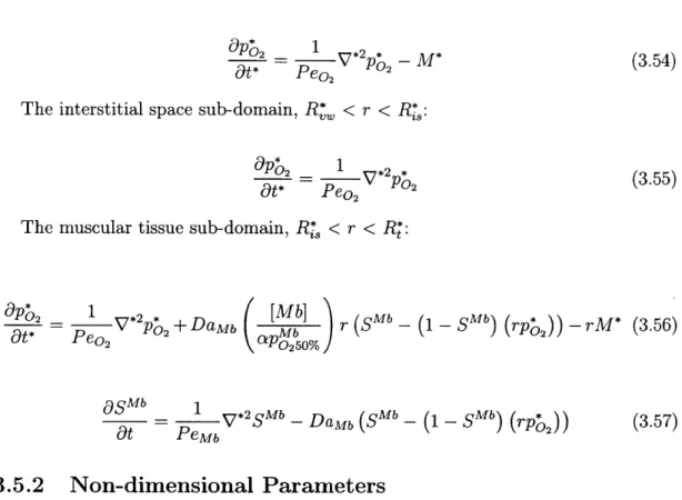
equations are succinctly presented in subsection 3.5.1 (alongside the dimensionless equations for the fluid mechanics). For a detailed derivation and explanation of the non-dimensional parameters, refer to Appendix B and Chapter 5, section ??, respectively.

3.3.1

Oxygen Species Transport: Boundary Conditions

The boundary conditions for the oxygen transport equations result from periodi-city of the domain and an oxygen flux constraint (e.g. analogous to that of a heat flux boundary condition).

The periodic boundary condition at inlet and outlet are enforced in a similar manner to those of the fluid mechanics. For the capillary domain, the advection and diffusion terms are approximated at the inlet using information from the outlet and preceding points (as required). The outlet is set equal to the inlet by definition. (This enforcement of the boundary conditions is one way to construct it. Many other methods exist, and this method was chosen for its simplicity).

Across non-periodic boundaries, a normal flux constraint on the oxygen partial pressure is applied. It is mathematically expressed as:

(aDo2Vpo2 -ft)1 = - (aDo2Vpo2 -,h) 12 (3.24) where 1 and 12 indicate regions 1 and 2 (e.g. cytoplasm region and blood plasma

region).

First, in the capillary, vascullar wall, interstitial space, and tissue sub-domains, the gradient exists only in the y-direction at the intersections of both domains (see Figure 3-1). This boundary condition is expressed as:

aD

_y

_dy)2

d

However, across the RBC membrane, the normal derivative is in both the x and y-directions. The boundary condition for this region is

[(ceDo2 Vpo2 -) (X- X(s))] - [(aDo2 VPo2 -h) 6 - X(s))] (3.26)

where [-]p indications the blood plasma region and [.]c indicates the cytoplasm region. For the detailed, dimensionless treatment of equation (3.26), refer to Appendix E.

3.4

Red Blood Cell Membrane Mechanics and

Inte-ractions with the Microcirculation

The RBC membrane is modeled as a segmented beam. It is suspended in the blood plasma and surrounds the cellular cytoplasm. Motion of these surrounding fluids impart momentum to the membrane and the membrane provides a resistance to motion in return. The interaction is a two-way reaction, i.e. the fluid motion affects the RBC membrane motion and the RBC membrane motion affects the motion of the

fluid.

In order to capture this interaction, a body force model is used. The RBC mem-brane is assumed infinitely thin and is massless, thus it acts as a solid boundary which separates two distinct fluid regions. Given that it is extensible (can move and deform), not only must it be integrated into the fluid equations of motion as a body force, but it must also have unique boundary conditions that update its location while enforcing the zero-velocity boundary condition in the reference frame of the local RBC membrane location.

The body force term

f

dFt dF

f

fy