Analytical crashworthiness methods applied to composite structures

Analytical Crashworthiness Methods Applied to Composite Structures

by

Keith W. Lehnhardt

B.S., United States Naval Academy, 1991

Submitted to the Department of Ocean Engineering and the Department of Mechanical

Engineering in Partial Fulfillment of the Requirements for the Degrees of

Naval Engineer

and

Master of Science in Mechanical Engineering

at the

MASSACHUSETTS INSTITUTE OF TECHNOLOGY

June 1999

C1999 Keith W. Lehnhardt. All rights reserved.

The Author hereby grants to MIT permission to reproduce and to distribute publicly paper and electronic copies of this thesis document in whole or in part

Sianature of

Author_---Department of Ocean Engineering

13 May, 1999 Certified by

Tomasz Wierzbicki Professor of Applied Mechanics Thesis Supervisor

Certified by_

James H. Williams, Jr. SEPTE Professor of Engineering -- Thesis Reader

Accepted by

A _{Art Baggeroer} Ford Professor of Engineering Chairman, Departmental Comp" ate Studies

Accepted by

Ain A. Sonin Chairman, Departmental Committee on Graduate Studies

Analytical Crashworthiness Methods Applied to Composite Structures

by

Keith W. Lehnhardt

Submitted to the Department of Ocean Engineering on 13 May 1999, in partial fulfillment of the

requirements for the degrees of Naval Engineer

and

Master of Science in Mechanical Engineering

Abstract

Several shell deformation models are developed for use in crashworthiness analysis of rotationally symmetric structures. These models use analytical techniques to predict the crushing force versus axial crush distance characteristics of both a rigid-plastic, hemispherical shell and an elastic, cylindrical shell loaded axially by a rigid flat plate. Additional methods are proposed to determine the effects of cutout sections and internal stiffening members on the crushing force capacity of the shells. These proposed methods are applied to determine the energy absorption capability of the composite/metal nose structure of a mini submarine subjected to a head-on impact with a flat rigid wall. The nose structure is composed of a stiffened composite shell that covers and is attached to the metal, forward, hemispherical portion of the pressure hull. The complex structure is simplified to a rotationally symmetric shell model and modified to account for the effects of stiffening elements and cutout sections. Laminated plate theory, a progressive composite failure method, and the models developed are then used to determine the structure's energy absorption capacity. The fairing structure is determined to be capable of absorbing the kinetic energy associated with an impact from an initial vehicle speed of 7.5 knots. Further, the entire nose structure (the fairing and forward pressure hull) is predicted to be able to absorb the kinetic energy from a 26.4 knot vehicle impact.

Thesis Supervisor: Tomasz Wierzbicki Title: Professor of Applied Mechanics Thesis Supervisor: James H. Williams, Jr. Title: SEPTE Professor of Engineering

Contents

1 Introduction

2 Development and Discussion of Analysis Tools 2.1 Crushing Response of a Hemispherical Shell Between

2.1.1 Prior Research

2.1.2 Deformation Process . . . . 2.1.3 Deformation Model . . . . 2.2 Derivation of Cylindrical Tube Equation 2.2.1 Prior Research . . . . 2.2.2 Deformation Process . . . . 2.2.3 Deformation Model . . . . 2.2.4 Correction for Open Sections 2.2.5 Effect of Shell Stiffeners...

3 Modeling and Analysis of ASDS 3.1 ASDS Modeling . . . . 3.1.1 Actual Structure . . . . 3.1.2 Simplified Model . . . . 3.2 Analysis . . . . 3.2.1 Impact sequence . . Rigid Plates . . . . . 1 1 3.2.2 Sonar Dome . . . . 3.2.3 3.2.4

Frustum Section of Nose Shell . . Cylindrical Section of Nose Shell

8 11

11

Composite Shell Structure

12 13 20 20 21 22 26 32 34 34 34 36 38 38 39 42 47

3.2.5 Analysis of Forward Hemi-head of Pressure Hull . . . . 47 3.2.6 Kinetic Energy Calculations . . . . 48 3.3 R esults . . . 51

4 Summary and Conclusions 54

4.1 Areas Additional for Study . . . 55

A Sonar Dome Analysis 59

B Frustum Section Analysis 70

C Cylindrical Section Analysis 85

D Stiffener Analysis 100

List of Tables

3.1 Properties of Materials Used in ASDS Nose Fairng. . . . 36

3.2 Comparison of Actual and Modeled Sonar Dome Dimensions. . . . 38

3.3 Comparison of Actual and Modeled Nose Shell Section Parameters. . . . 39

List of Figures

1-1 External Isometric View of the ASDS . . . . 9

2-1 Geometry of Hemispherical Deformation Model . . . . . 12

2-2 Membrane Stress and Fully Plastic Bending Moment Representation for Material having Differing Compressive and Tensile Flow Stresses. . . . . 15

2-3 Deformation of Surface BCD. . . . . 17

2-4 Deformation Model for Cylindrical Thin-walled Structure. . . . . 21

2-5 Detailed View of the Deformed Cylinder Section. . . . . 23

2-6 Top View of Hemispherical Dome with a Single Circular Cutout Section. . . . . . 28

2-7 Geometrical Relationship of Parameters Used in the Derivation of the Correction Factor for Open Sections in a Dome Structure (side view). . . . . 29

2-8 Geometrical Relationship of Parameters Used in the Derivation of the Correction Factor for Open Sections in a Dome Structure (top view). . . . 30

2-9 Stiffener Smearing Process. . . . 32

3-1 The Actual ASDS Nose Fairing Structure Showing Internal Components (Viewed from Aft Looking Forward). . . . 35

3-2 Model of ASDS Forward Section (Dimensions in meters). . . . 37

3-3 Compressive and Tensile Stress vs Strain Estimates Calculated using the Pro-gressive Failure M ethod. . . . . 42

3-4 Crushing Force and Cumulative Energy Absorption as a Function of Axial Dis-placement for the Sonar Dome. . . . . 43

3-5 Transverse Young's Modulus Variations with Pure Tensile, Transverse Strain for

Frustum Section. . . . . 44

3-6 Flexural Strain to Axial Crush Distance Relationships for the 0 Degree Oriented Plys in the Frustum Laminate. . . . . 45

3-7 Flexural Young's Modulus and Laminate Thickness Variation with Axial Crush Distance of the Frustum Section. . . . . 46

3-8 Crushing Load and Cumulative Energy Absorption Characteristics of the Frus-tum Section. . . . . 46

3-9 Crushing Force and Cumulative Energy Absorption of the Cylinder Section of the N ose Shell. . . . 48

3-10 Crushing Force and Cumulative Energy Absorption for the Forward Pressure H ull Hem i-head. . . . . 49

3-11 Description of Standard Submarine Weight Terms . . . . 49

3-12 Dimensions Used During Added Mass Calculations . . . . 51

3-13 Vehicle Kinetic Energy for Various Speeds. . . . . 52

3-14 Crushing Force Profile for the Entire Deformation Process. . . . . 53

Chapter 1

Introduction

The Advanced Seal Delivery System (ASDS) (Figure (1-1)) is a highly sophisticated, mini-submarine 19.8 m long that displaces 60 metric tons submerged. It is designed to transport a team of Navy SEALs from a host submarine to a tactical point of insertion and back. While the transported SEALs are a formidable offense weapon, the ASDS itself has no offensive or defensive capabilities and must rely on stealth and its ability to "hide" in the water column to ensure the safe transport of its personnel. As such, the ASDS will be operating in close proximity to the ocean bottom in order to mask its underwater signature. This near bottom operating strategy presents some problems, however. The most pressing of these is the increased risk of impact with submerged objects or structures. For the safety of the embarked crew, it is paramount that a determination be made as to the crashworthiness of the ASDS and whether operational restrictions need to be imposed. In effect, a safety envelope needs to be developed which takes into account the depth, bottom type and impact angle to give a maximum safe operating speed. A natural starting point for this analysis is to look at how a front end impact will affect the forward structure of the vessel. This analysis, however, presents no small task. The complexity of this problem quickly becomes apparent when the structure types and problem variables are viewed:

9 The structure of the nose section consists of various composite materials and steel in-cluding: glass woven cloth, carbon cloth, kevlar, vinylester, rubber, syntactic foam, and

Tail Section

Aft Body

Access to Thrusters

Access to Anchor

Mid Body

Nose Section

Access to Thrusters

_{Gas Bottles}

Access to Anchor

G.

Battery Bottle Sonar Window

Figure 1-1: External Isometric View of the ASDS

9 The variables of the problem include: depth, impact angle, speed, and bottom type.

Additionally, the interaction of the structural material and modes of failure during defor-mation and fracture are not well understood or predictable to a high degree of accuracy. In light of these complexities, using model testing to develop some empirical means of relating the structural behavior during a collision to key parameters such as impact angle, velocity, or crush distance would be the optimal analysis tool. However, due to the cost associated with such tests, this method is not feasible. Moving to the other end of the spectrum, a computer simulated "crash" test of the ASDS could, in theory, be used to ascertain the desired safety envelope at a substantially cheaper price and in an accelerated time frame. While modeling the full ASDS via computer simulation seems plausible on the surface, a little digging reveals that even the most sophisticated computer tools have not evolved far enough to accurately predict impact responses for such complex, composite/metal structures. With this in mind, it is apparent that neither model testing nor computer simulation alone can solve this problem.

A middle road between these methods may be the required path. In effect, a combination of

structural simplification and computer and analytical modeling will be used to complete the analysis. With all of this said, the overall objective of the project will be to determine a safe impact speed for the vehicle such that during an impact the pressure hull will not rupture and

the crew will be able to survive the collision.

As a first step in solving the problem, this thesis will analyze the energy absorbing potential of the composite nose fairing and forward pressure hull hemi-head structures during a head-on impact with a rigid wall structure. While this impact scenario is idealized and likely never to occur during actual operations, it will serve as a worst case impact and best case energy absorption scenario. This will be a worst case impact from the stand point that all kinetic energy will be absorbed by the structure in the form of deformation. No energy will be absorbed by the impacted structure or be maintained as vehicle kinetic energy. This is a best case energy absorption scenario in that the impact will allow the full utilization of the bow structure to absorb energy before the pressure hull is impacted. The reasoning behind looking at such a case first, is to ascertain the maximum energy absorption potential of the composite structure.

This analysis will progress in three phases:

" Deformation model development.

" Structural modeling of the ASDS nose structure.

" Energy absorption analysis.

The models developed include deformation relationships for a rigid-plastic, hemispherical and an elastic, cylindrical shell loaded axially by a rigid flat plate. A method is also included to approximate the reduced load carrying capacity caused by cutouts in the shell structure. Next, the composite shell of the nose fairing will be modeled using simplified, rotationally symmetric shells (i.e.- cylinders, frustum, and hemispheres). Internal stiffening members are incorporated into the model by "smearing" the effective area of each stiffener across portions of the inner surface of the shell to increase the effective thickness of the structure. Cutouts in the shell for components, such as thruster doors, video equipment, and lights are also modeled. Finally, the deformation relationships developed will be applied to the corresponding sections of the model to produce a force verse displacement relationship of the structure as it is crushed axially by a rigid flat plate. The energy absorption capability of the entire structure will then be determined and translated into the vehicle speed needed to produce such an impact.

Chapter 2

Development and Discussion of

Analysis Tools

2.1

Crushing Response of a Hemispherical Shell Between Rigid

Plates

2.1.1

Prior Research

Much attention has been devoted to the study of the energy absorbing characteristics of thin-walled, metal, dome structures [1]-[7]. The problem of large deformations of rigid-plastic, spher-ical shells being compressed between rigid plates was first studied by Updike [1]. A simplified yield condition and geometry was used to obtain a sequence of limit loads, thus producing a force-displacement relationship valid from a displacement of a few shell thicknesses to about 1/10th the shell radius. Wierzbicki [4] used similar geometric and deformation assumptions to derive a force-deflection relationship based on the optimization of bending and membrane energies valid theoretically until the plate deflection reaches half the radius of the shell. Com-parison of [1] and [4] show that the force-displacement results predicted by each differ only slightly. Experimental testing of hemispherical shells was reported by Kitching [5] and Kin-head [51. Kitching et al studied the quasi-static loading of hemispherical shells and observed experimentally three different stages of deformation for shells with radius to thickness ratios ranging from 36 to 460. Later, Kinkead performed experimental testing on shells with radius

0

AO

Figure 2-1: Geometry of Hemispherical Deformation Model.

to thickness values ranging from 8 to 32 and identified two vice three deformation stages. The loading characteristic observed by Kinhead were compared to values predicted by the methods of [1] and [4] and large differences were found. Gupta [7] developed another prediction method using a rigid plastic analysis which relies on two calibration constants that must be determined from curve fits of experimental data. The method proposed by Gupta showed good correlation with experimental results. This analysis develops a means of predicting the load-compression relationship of hemispherical shells using a rigid plastic analysis technique with an emphasis on creating a simple, analytical model whose accuracy is improved over that proposed in [1] and [4]. The model developed will utilize the same deformation model used by [1] and [4], but calculate the membrane energy using a simple strain averaging method. Additionally, the re-sulting relationship will be capable of analyzing material with differing compressive and tensile stresses.

The spherical shell of radius R will be loaded from the top by a moving rigid plate with the base of the shell pinned to a fixed rigid plate. As the shell is loaded axially, a spherical dimple forms which is an inversion of the original shell curvature as shown in Figure (2-1). In this deformed state, surface AB remains rigid and undeformed. At point B, a circumferential plastic hinge increases the curvature of the shell, followed by rigid body translation between B and D and a reversal of curvature by the plastic hinge at D. The shell is subsequently unloaded and rigid body translation results on surface DE. As the shell deforms, the hinge circles at B and D move progressively outward. Deformation continues in this manner until the inverted portion of the shell at point E contacts the fixed rigid plate.

2.1.3 Deformation Model Geometry

This analysis begins with a look at the various geometrical relationships that can be attained from the deformation model in Figure (2-1). First, the radius to the center of the toroidal surface (a) and the displacement of the moving rigid plate (6) can be expressed in terms of the shell radius (R) and deformation angle

(#)

as

a = R sin #, and (2.1a)

6 = R(1 - cos #) (2.1b)

By differentiating Equations (2.1a) and (2.1b), the radial and axial velocities of the toroidal section and rigid plate become

da d#5 - = R(cos #)- , and (2.2) dt dt dS d#b -= R (sin #) (2.3) dt dt

By approximating cos

#(t)

using the first two terms of its Taylor expansion in Equation (2.1b) and rearranging, a simple equation relating the deformation angle to the rigid plate displacement can be deduced.

4

2= (2.4)

Turning now to the toroidal surface BCD, the average plastic hinge length (L) and toroidal surface area (A) can be calculated by the Equations (2.5a) and (2.5b).

L = 21ra, and (2.5a)

A = 47rra# (2.5b)

Additionally, the radial and rotational velocities of the plastic hinge at point B can be taken as

V =R- (2.6)

dt

dO _ V _Rdo(2.7)

dt r r dt

Finally, in order to simplify subsequent calculation, surface BCD will be approximated as a parabolic surface of the form

y 1 2 + r(1 -cos#) (2.8)

2 r sin

y

with the x and y axes oriented as shown in Figure (2.2.3).

Derivation of Membrane Stresses and Fully Plastic Bending Moment

Next, the membrane force (N) and fully plastic bending moment (M) relationships for a material having differing compressive (o-) and tensile (at) flow stresses will be developed. As shown in Figure (2-2), when ac

#

at the neutral axis will shift away from the geometrical

center of the cross section by an amount 7. By using the fact that the neutral axis of a specimen subjected to a bending moment is located where the membrane force (N) is equal to zero, we are able to calculate a general expression for q in terms of shell thickness (t), o-, and at as shown below

2+7f t- 77

N = O tdz - oUdz = 0 (2.9)

Figure 2-2: Membrane Stress and Fully Plastic Bending Moment Representation for Material having Differing Compressive and Tensile Flow Stresses.

(2.9) becomes

1 t a - t _(2.10)

t

20oc + -t

With a calculated, general expressions for N and Ml can be derived as follows:

N =

jO-dz

M = ]0 -tzdz]+ o-czdz

Note that the regions of membrane deformation are compressive in nature while the bending forces are both tensile and compressive. After integrating, substituting Equation (2.10) for r7, and setting a = 2 't , the total membrane force and fully plastic bending moments become

N = o-ct (2.11)

Al = I-ct2 - act2 (2.12)

2 -c + -t 4

In order verify the validity of Equations (2.11) and (2.12), -c can be set equal to ot which results in a symmetric stress profile throughout the specimen. In such a case Equations (2.11) and (2.12) reduce to the standard expressions for the fully plastic membrane force and bending moment.

Energy Balance

The principle of virtual velocities will be used to relate the rate at which energy is being introduced to the system to the rate at which it is being absorbed. Equation (2.13) states that the rate at which energy is applied to the shell must exactly match the rate at which it is being absorbed by the bending and membrane effects in the shell.

(1) (2) (3)

d6 dEb dEm

P -- + (2.13)

dt dt dt

The remainder of this section will further develop each of the terms in Equation (2.13). Starting first with the left hand side of Equation (2.13), term (1) can be rewritten in a different form by using Equation (2.3) as follows

P- = PR sin p-- (2.14)

dt dt

The second term of Equation (2.13) represents the rate at which energy is absorbed by the shell due to bending processes. Using the deformation model shown in Figure (2-1), it is plainly seen that bending energy will be absorbed at two discrete locations - plastic hinges B and D. This component can be quantified by the following expression

dEb dL

dt = FMDL (2.15a)

i=B,D

Equation (2.15a) can be further simplified by making the following assertions

" the magnitudes of the bending moment and rate of angular rotation at hinges B and D are equal.

" the total hinge length Li can be rewritten as 2L (where L is the average hinge

i=B,D

D C Ci Di C D B

Figure 2-3: Deformation of Surface BCD.

Using these simplifications and Equations (2.1a), (2.5a), and (2.7), Equation (2.15a) can be expressed in the following form:

dEb =47rR2 sin # Mdo _(2.16)

dt r dt

The final term in Equation (2.13) accounts for the membrane energy dissipated on surface BCD and can be written as:

dEm = NA-

(2.17)

dt dt

where - is the instantaneous rate of strain experienced by surface BCD. As a simplification, the average strain rate, dep, _dt will be used in place of the instantaneous strain rate. Figure (2-3) shows a detailed view of the deforming surface BCD. The average strain of this surface will be calculated by dividing the surface into two subsurfaces, calculating the average strain on each, and then averaging the strains from each region to get the final average strain. This

statement can be expressed mathematically as

aav

= ""

+ e11""

(2.18)

where ela and 6IIav are the average strains experienced as surfaces BC, (region 1) and C0D0 (region 2) deform to BCand CD respectively. Looking first at region I, the strain can be written in terms of initial and final curvatures of the BC.

EI = 6If - 6jo = I () - (2.19a)

In general, the average strain in region I can be formulated as:

1 f"S"l4

lay = s _{r sin} n 0 s]I

Edx

(2.20)

#

JO

Upon substitution of Equation (2.19a), integration and simplification, Equation (2.20) reduces to

6Iy = -42 (2.21)

3

The strain in region II requires an additional step to calculate. While the strain in region I is purely compressive for the entire deformation, the strain in region II is initially compressive for the first part of deformation and then tensile for the remainder of the deformation. So, the average strain will be calculated for the compressive phase as surface C0D0 is deformed to an intermediate flat surface CiDi and also for the tensile phase as the shell further deforms to surface CD. With this, the average strain in region II can be calculated in the same manner

as in region I. The details of the calculation follow.

EIIan = IIavcompressive + EIIavtenssie

IIav rsin E Ifcompressive - lcompressive) + (IIftensile - EII0 '

*~)]

dx

SI

~~

Iin r i0

CilaI = snqjrsino [(!2 -

o)

+

(o

()) dx

EIIa, = 2- (2.22)

With the average strain calculated in both regions, we can now determine the average strain of the entire surface BCD by substituting Equations (2.21) and (2.22) into Equation (2.18). Subsequently, the average strain rate can be calculated by simple differentiation of the average strain as follows. 12 Eav = 2 (2.23) 2 d6av Odo _(2.24) dt di

Now a final expression for the rate at which energy is absorbed by membrane forces can be realized by substituting Equations (2.5b), (2.1a) and (2.24) into Equation (2.17).

dEm = _{4rrNR sin @&2}

(2.25)

dt dt

New expressions have now been formulated for each term in Equation (2.13). By substituting the new expressions (Equations (2.14), (2.16), and (2.25)) into Equation (2.13) and solving for

the instantaneous crushing force (P), the following result is obtained

P= 4 r (RM+NrY) (2.26)

Further, the mean crushing force (P) can be calculated and minimized with respect to the

toroidal radius (r) to obtain an optimal toroidal radius.

- P R N P =2 - +r-2 (2.27) 27rMAI r Ml

dP

₂

_N

_R

0

dr = kM r2 N

4

(2.28) r o J RM

By substituting the optimal toroidal radius back into Equation (2.27) and using the fact that at the optimal radius the membrane and bending contributions are equal, the mean crushing force can be expressed more simply as

- N

Port = 4#R RA (2.29)

Equation (2.29) can be rewritten in terms of plate displacement and shell thickness by using

Equations (2.4), (2.11), and (2.12).

26 (2.30)

P5opt = 8 _(2.30

ta

Finally, the optimal instantaneous crushing force becomes

Port = 47tdoca t26o (2.31)

2.2

Derivation of Cylindrical Tube Equation

2.2.1 Prior Research

The deformation and energy absorption characteristics of thin-walled, composite, cylindrical shells have been studies for many years by many researchers. [8]-[15]. Farley [10]-[13] and Hull

[14]

have performed extensive testing on composite shell samples composed of various mate-rials using different lay-up conditions. Both quasi-static and dynamic loading situations were investigated. These studies did much to further the knowledge base in the areas of determining crushing modes and their controlling mechanisms. They also showed that there was no explicit set of rules that could be generalized for all composites types. Material lay-up pattern, crushing speed, fiber volume fraction, and radius to laminate thickness ratio all play key roles in deter-mining the deformation characteristics of the shell. From these studies, complicated numerical models have been established for use in predicting the failure of very simple composite struc-tures. The degree of success realized by these models has varied in even simple situations. The vast majority of the work described has been directed toward understanding the deformation of composites on the micro- and macroscopic scales. Hanefi and Wierzbicki [15] took a more global approach to a similar deformation problem. They developed a simple model that was used to predict the energy absorption characteristics of a combined metallic/composite tube structure in axial compression. The model coupled a rigid plastic analysis of the metal tube with a compressive perfectly plastic and tensile elastic analysis of the composite material. The

Figure 2-4: Deformation Model for Cylindrical Thin-walled Structure.

predicted results matched well with experimental data. In this analysis, a global failure ap-proach will also be taken. A deformation model will be developed using elastic principles to determine the force deflection and energy deflection characteristics of a thin-walled, cylindrical shell loaded axially. Bending and in-plane stiffnesses will be step-wise varied to account for stiffness variations as plys fail within the structure. Finally, a simple result will be established for a material exhibiting constant and identical flexural and inplane stiffness properties.

2.2.2

Deformation Process

Figure 2-4 shows a representation of two buckling lobes of the cylinder during deformation where 6 denotes the axial crush distance, a is the radius of the cylinder, and 2H is the half

- - - - - -

-- -- -- --- - - - -- -- -- --

-length of the buckling lobe generated. As the cylinder is crushed axially by a distance 6, the cylinder will form an axisymmetric, elastic buckling pattern with a wave length equal to 2H. Deformation takes place both in the form of bending and circumferential strain. The material will behave elastically until its elastic limits are reached with subsequent deformation occurring with the material in a progressively degraded state. The material degradation takes place through a step-wise reduction of the material's flexural and circumferential elastic moduli and material thickness. The process continues progressively through all buckling lobes formed.

2.2.3 Deformation Model

The principle of virtual work (Equation (2.32)) will be used as the starting relationship from which to derive an expression relating the crushing force (P) to the axial crush distance (6). Equation (2.32) states that the energy applied to the cylinder through an external force (1) must be exactly equal to the energy absorbed by the structure in the form of circumferential

(2) and bending (3) strains.

(1) (2) (3)

Pd6 = (o-odeo + o-,de )dV (2.32)

c- = Eeo and a-, = Ee, (2.33)

Pd6 = j(Eeodeo + Eedex )dV (2.34)

Because the deformation will be elastic, Equation (2.32) can be simplified using the elastic relationships between stress and strain (Equation (2.33)) to obtain Equation (2.34). Figure (2-5) shows a detailed view of the deformation of a single buckling lobe with parameters pertinent to the analysis labeled. Using this figure, expressions can be derived in terms of the variables shown for the incremental volume (dV), strains (6s, and 60), and incremental strains (del and dEo). First, inextensibility will be assumed for the shell as it buckles, making dV constant over the deformation process and having the following value:

X R a _H -t/2 w 0-x I

/

Figure 2-5: Detailed View of the Deformed Cylinder Section. t/2

z

Next, the circumferential strain can be expressed as the ratio of the outward deflection of the shell (w) to the original shell radius. The actual deflection is measured from the original surface of the shell to the deformed surface and varies from 0 at the being of the lobe to a maximum value of wo at the midpoint, and then back to 0 at the end of the lobe. In order to simplify future calculations, a linear deflection profile (w(x') = Hwo) is used to approximate the actual

deflection profile as shown in Figure (2-5). Using this linear relationship, 6o and deo can be expressed as w x' E = W (2.36) a aH deo = X dwo (2.37) aH

The bending strain component can be determined by using the curvature of the shell section (r,) and the position within the thickness of the material (z) as is shown in Equation (2.38). This variation of the bending strain throughout the shell thickness will be assumed linear with maximums occurring at 1 and -1 and no strain occurring at the mid-plane. Further, plane sections will remain plane as shell curvature increases.

Ex = z = - (2.38)

R

However, the radius of curvature (R) is related to the half lobe length and the maximum circumferential deflection by Equation (2.39)

R 2 -(R - )2 = 2 _W2

H2

R= (2.39)

Substitution of Equation (2.39) into Equation (2.38) yields the final expressions for e. and dex

(Equations (2.40) and (2.41)).

2z

EX= H2WO (2.40)

2z

Now, Equations (2.35)-(2.37) and (2.40) can be substituted back into Equation (2.34) to obtain the following:

Pdb = (4aYi H Em(x')2dx' + Ff (4raH) 2 z2dz _w

0dwo (2.42)

If the flexural and membrane Young's moduli can be assumed equal and constant throughout the deformation process, Equation (2.42) can be further simplified to Equation (2.43 ).

4

FtH

atB~

Pd6 = -irE - + H3 w_{3 [a HT}3 0dwo0 (2.43)

Previous work [18] has proven that the elastic, buckling lobe length of a cylinder can be related to the shell radius and thickness by

2H = 1.72Vai

H ~

Vat

(2.44)

Using Equation (2.44), Equation (??) can be reduced to

4 t /at Pd6 -7rE 3 1a Pdo Pdo

at

3 + I wodwo atVatI 4 -7rE _{t - t} -wodwo 3 ta +ta 8 t ~-rEt -wodwo 3 a (2.45)

A final simplification can be made to Equation (2.45) by relating 6 to w,. Using Figure (2-5) the following geometric relationships can be generated.

sin(a) W=

H (2.46)

(2.47)

By squaring and adding Equations (2.46) and (2.47), the relationships are combined in the

following form

-- 2

1 1(2.48)=

I""

+

H 2H

After differentiating, rearranging and substituting Equation (2.44), the desired relationship is achieved

6' d6

w0dw2

2

This expression can now be substituted back into Equation (2.45) to obtain the final expression relating the crushing force applied to the axial deflection of the cylinder.

P(6) ~ 7rE t2 t t (2.49)

As previously states, Equation (2.49) applies to materials with equal and constant flexural and circumferential Young's moduli. If these conditions are not met, the more general expression

(Equation (2.42)) must be used.

2.2.4 Correction for Open Sections

Open sections or cutouts in a shell will effectively reduce the load required to deform the shell in the local region of the cutout. These cutouts could even change the local deformation mode of the structure or change the order in which the overall structure deforms. For simplicity, this analysis will include only the reduction in loading capacity for several reasons. The relationships previously developed, Equations (2.26) and (2.49), are valid only for the failure modes assumed; so, a change in failure modes (i.e.- from axisymmetric shell yielding to lobar buckling for ex-ample) will not be captured here in. While this seems like a fairly unreasonable assumption, the reader is reminded that the objective of this analysis is to determine the maximum energy absorption capability of the structure. The development of Equations (2.31) and (2.49) assume failure modes which produce this maximum. So, a shift to a different mode would produce a lower energy absorption. With the assumption that the failure mode remains unchanged at the cutouts, it does not make sense to consider the order in which parts of the structure collapse because the same amount of energy will be absorbed regardless of the collapse sequence. So, the

only effect that will be considered is the reduction of strength caused by the loss of material. This effect will be approximated by multiplying the applied load of an intact shell by a reduc-tion factor in the local vicinity of the cutout. This reducreduc-tion factor will be proporreduc-tional to the remaining shell area divided by the material present in an intact shell of the same dimensions

(Equation (2.50))

F(6)corrected = F(6)uncorrectede(6) where

6() = _{(Acomplete shell(} 6_{) - Aremoved material(}6_{)) (2.50)} 1 Acomplete shell W)

While this area ratio is part of the reduction effect, it does not capture all aspects. Other factors, such as cutout geometry, affect the load carrying capacity of the structure around the cutout. While these other effects are recognizable, a theoretical derivation of their effect is impractical. This effect must be determined experimentally. The experimental correction factor would be used to match experimental test data with theoretical predictions and is expressed as ( in Equation (2.50). Since no experimental calibration was done during the course of this thesis, ( will be set equal to 1 until future evaluation determines its correct value.

Hemispherical Dome

For the hemispherical dome, the cutout sections will be assumed to be circular with diameter D as shown in Figure (2-6). From Figure (2-6) it is apparent that the correction factor can be stated in terms of the average plastic hinge radius (a(6)) and angle

#(6)

as follows:

(Average Hinge Diameter-Length of Open Section) \\

Average Hinge Diameter

)hemisphere

= 27ra) - (6)a(6)

)hemisphere

= b- hemisphere (2.51)

27raQ5)27)

The task now becomes to express

#(6)

in terms of known quantities. Figures (2-7) and (2-8) show more detailed views of the side and top of the shell respectively with pertinent dimensions labeled in each figure.

a

(a < r)A

_D

a A2 (r.< a<r, ) -A-r___,__,Dcos(6

)

r

Figure 2-7: Geometrical Relationship of Parameters Used in the Derivation of the Correction Factor for Open Sections in a Dome Structure (side view).

From these figures, the following geometric relationships can be established:

Al = r,+Dcos0-a(6) A2 = Al cos 0 A3 = D-A2 D D A4 =

--

A3=A2--2 2 A5 = ( -) A42 (2.52)

#(6)

can now be expressed in terms of the initial radius at which the cutout is encountered (ro),

cutout diameter (D), cutout inclination angle (0), and average plastic hinge radius as shown in Equation (2.53).

a(8)

A5 A4

D/2

Figure 2-8: Geometrical Relationship of Parameters Used in the Derivation of the Correction Factor for Open Sections in a Dome Structure (top view).

(A5

#(6) _{= 2 arcsin (A-(6)}

ro,+ Dcos 0-a(6)

D

_r +D cos 0-a(±)L

#(6) = 2 arcsin a(6) (2.53)

(V/roDcs~(6) r+Dco Oa(6)))(.3

Next, a(6) can be related directly to the radius of the hemisphere (R) and the crush distance of the shell (6) by the following:

a(6) = VR 2 - (R - 6)2 = V6(2R- 6) (2.54)

Finally, substitution of Equation (2.54) into (2.53) and the result into (2.51) yields the desired result for the correction factor (Equation (2.55))

(ro+Dcos-x62-6) (D (ro+DcosO -6(2R6)

e(6) = [1 - arcsin C6(2R - 6) 0hemisphere

(2.55)

Cylindrical Shell

The same principles described in Section (2.2.4) will also be used to estimate the effect of cutout sections in the cylindrical section with the exception that the cutout shape will be much simpler. The cutouts in the cylindrical section will be rectangular in shape, and thus, the material removed will not vary with axial crush distance. So, using Equation (2.50) and again assuming that (= 1, the correction factor of the cylinder can be expressed as

= 27ra -na =1 where (2.56)

27ra 27r

n = Number of cutouts

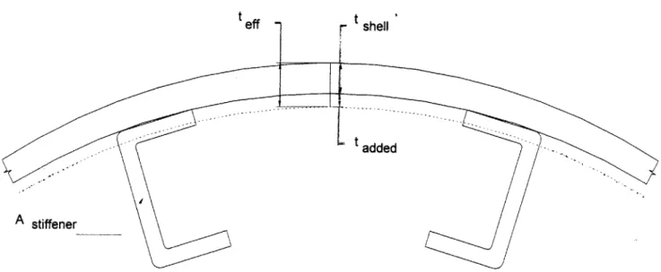
t

eff

_{t shell}

t added

A stiffener

Figure 2-9: Stiffener Smearing Process.

2.2.5 Effect of Shell Stiffeners

The energy dissipation effects of shell stiffeners can be taken into account using Equations (2.31) and (2.49) by assuming that these structural members are "smeared" across the surface of the shell so as to produce a new effective shell thickness. This process is illustrated in Figure (2-9). If the material properties of the stiffeners are identical to those of the shell material, their cross sectional area is distributed across the surface of the shell such that the new effective thickness

(teff) can be determined by the following expression

n

E Ai

teff = tshell + i=1 (2.57)

27a

where Ai is the cross sectional area of the ith stiffener, n is the total number of stiffeners, a is the shell radius, and tshell is the shell thickness. If the shell and stiffener materials have different properties, the force distribution over the effective cross section must be made consistent with the force distribution prior to the "smearing" process by using the following relationship

By substituting the appropriate relationships and assuming that Peff will be calculated using the shell properties, Equation (2.58) can be written as

n

2_{7ratef fEshelle =} 2

7atshelIEsheIte + AjEie

i=1

which can be solved to determine the effective shell thickness

tef f = tshell + 27aE1 Ai E (2.59)

Chapter 3

Modeling and Analysis of ASDS

Composite Shell Structure

With the analysis tools developed, focus now shifts to the modeling and analysis phase of the project. First, a model will be developed for the actual ASDS nose fairing structure and forward hemi-head of the pressure hull using simple, rotationally symmetric, geometric shapes for the shell. Stiffeners and cutout sections will be incorporated using the techniques discussed in Section (2). Next, the analysis tools developed in Section (2) will be applied to determine the crushing force to axial crush distance relationship and energy absorption capability of the structure. Finally, a maximum impact speed will be calculated by equating the energy absorbed in the collision to the kinetic energy possessed by the vehicle just prior to the impact.

3.1

ASDS Modeling

3.1.1 Actual Structure

The forward portion of the ASDS consists of a hemispherical pressure hull and a composite fairing structure. The hemispherical pressure hull section is constructed of HY-80 steel and is welded to the cylindrical portion of the hull to form a water tight boundary. The ASDS nose fairing (see Figure (3-1)) is a composite structure attached to the forward end of the pressure hull by eight titanium clevises. The structure has an overall length of 2.94 m and a

Figure 3-1: The Actual ASDS Nose Fairing Structure Showing Internal Components (Viewed from Aft Looking Forward).

Property A B C D E Ei (x 106 psi) 3 11.6 4.7 .0013 16.4 E2 (x 106 psi) 2.7 10.6 4.7 .0013 16.4 E3 (x 10' psi) .55 .37 .45 - -Vi,2 .15 .124 .15 .499 .31 Fiber Content .5 .5 .5 - -Tensile Strength Axial (X) (ksi) 39.1 75 56 - 125 Transverse(Y) (ksi) 39.1 75 56 - 125 Compressive Strength Axial (X') (ksi) 33.8 68 14 - 125 Transverse (Y') (ksi) 33.8 68 14 - 125

Shear Strength (S) (ksi) 9.41 7.5 4.5 - 77

A-E-Glass (1583)/Epoxy (7780) woven cloth

B-Carbon woven cloth (6K 5HS satin weave IM7) C-Kevlar (K285)/ epoxy (7714) woven cloth D-Rubber core material

E-Titanium clevise material (Ti 6A1-4V)

Table 3.1: Properties of Materials Used in ASDS Nose Fairng.

pseudo-rectangular cross section with maximum dimensions of 2.21 m high and 2.06 m wide. The structure itself consists of an outer shell constructed from E-Glass (1583) /Epoxy (7780) preimpregnated (prepreg) woven cloth in a single mold process. Internally, the shell is stiffened by a network of longitudinal and transverse woven carbon cloth (6K 5HS Satin Weave IM7) beams which are bolted to the shell and interconnected by titanium clevis fittings. Attached to the front end of the shell is a sonar dome comprised of a BFGoodrich Rho-Cor material system. This system consists of Kevlar (K285)/Epoxy (7714) prepreg woven cloth with a rubber core material. The properties for the various material systems described are contained in Table (3.1). Cutouts have been made in shell and the sonar dome to accommodate such equipment as thrusters, the forward anchor, lights and video cameras.

3.1.2

Simplified Model

The actual structural design of the ASDS had to be simplified to rotationally symmetric shapes before the analysis tools developed in Section (2) could be applied. A representation of the model developed is shown in Figure (3-2). For the forward pressure hull, no modeling idealizations needed to be made since the structure was already rotationally symmetric and

Camera Cutout 1. 36 -. 95 .63-28 DIA .91 R - 8 11--.07 R .71

Thruster Door Cut

1.13 .9948'

Anchor-'Light Cutou

Transverse Beams Forward Pressure Hull Hemi-head

Figure 3-2: Model of ASDS Forward Section (Dimensions in meters).

hemispherical in shape. The pressure hull has a .99 m radius and an undisclosed thickness. The actual thickness of the structure is held as confidential by the U.S. Navy so as not to reveal the operational diving depth of the vessel. For this analysis, a notional thickness of 19 mm will be used. The sonar dome was modeled as a spherical dome section using the axial depth of the actual sonar dome and a base radius equal to the average of the height and width of the actual sonar dome. The thickness and lay-up construction was taken to be that of the actual structure. Three cutout sections simulating the locations of the camera and lights were located on the model 1200 apart at the same radial distance. The actual and model sonar dome dimensions are summarized in Table (3.2). The shell structure was modeled using a combination of a frustum for the forward portion of the shell that transitions into the sonar dome and a stiffened cylinder for the after section. The radius of the cylindrical section was taken to be the average of the maximum height and width of the actual structure. The frustum was used as a transition section between the sonar dome and the cylindrical section and uses the corresponding radius at each end to fix its dimensions. For the frustum section, the shell thickness was taken to be that of the actual material. The thickness of the cylindrical section was taken to be an effective thickness calculated using Equation (2.59) to account for the added structural stiffness of the longitudinal carbon beams. The transverse beams were not utilized

Actual Parameter Model .64 Axial Depth (m) .635 1.91 Height (m) -1.75 Width (m) -1.83 Average (m) -- Radius (m) .91 9.6 Thickness (mm) 9.6 Camera Cutout .28 Diameter (m) .28 00 Orientation 00 .71 Radial Distance (m) .71 Light Cutout 1 .28 Diameter (m) .28 -1470 Orientation -1200 .72 Radial Distance .71 Light Cutout 2 .28 Diameter (m) .28 1480 Orientation 1200 .69 Radial Distance .71

Table 3.2: Comparison of Actual and Modeled Sonar Dome Dimensions.

in the effective thickness calculation because their energy absorption in an orthogonal impact is would be minimal. Instead, these beams were used to define nodal points for buckling waves. Table (3.3) summarizes the actual and modeled dimensions of the shell section. Two cutout sections 1.13 m high by .81 m wide were included in the cylindrical section to account for the openings created by the forward thruster doors. (It is assumed that during a collision imminent situation, the thruster doors would be open and the thrusters in use.) Additionally, the titanium clevises (used to attach the internal beams together and to the pressure hull) and the anchor were treated as rigid objects.

3.2

Analysis

3.2.1 Impact sequence

As stated previously in Section (1), this analysis will investigate an head-on impact with a flat, rigid wall. Structural deformation will initiate at the bow as the sonar dome is impacted first. The deformation will progress .635 m through the sonar dome, .95 m through the frustum

Actual Parameter Model Cylindrical Section 1.36 Length (m) 1.36 2.21 Height (m) 2.06 Width (m) 2.14 Average - Radius (m) 1.07 12.8 Thickness (mm) 35 Frustral Section .95 Length (m) .95 - Fwd Radius (m) .91

(Sonar Dome Radius)

- Aft Radius (m) 1.07

(Cylinder Section Radius)

10.1 Thickness (mm) 10.1

Table 3.3: Comparison of Actual and Modeled Nose Shell Section Parameters.

section of the nose shell, and .18 m into the cylindrical section before the anchor makes contact with the wall. At this point, some of the crushing load is transferred to the pressure hull via the anchor and simultaneous deformation of the cylindrical section and the pressure hull results for another .66 m. The deformation process ends when the after most transverse beams and titanium cleaves make contact with the wall.

3.2.2 Sonar Dome

Equation (2.31) will be used to determine the crushing force required to deform the structure throughout the progressive crushing of the sonar dome. Implicit in the use of this equation is that the structure can be modeled using rigid-plastic techniques. While it is understood that in general composite structures behave in a more brittle than ductile way, kevlar composites have been shown to buckle under axial loading in modes similar to those seen in metal structures [19]. This behavior coupled with the fact that the structure has a rubber core was used to justify the use of this analysis technique on this component.

The sonar dome is composed of 22 plys of kevlar cloth laid-up symmetrically sandwiching a 3.81 mm rubber core ([90, 0]5, 0, rubber core, 0, [90, 0]5) for a total laminate thickness of 9.4 mm. The compressive and tensile flow stresses were calculated using a combination of laminated plate theory and a progressive failure analysis [21]. The detailed calculations are shown in

Appendix (A) and, for brevity sake, only an summary of the process and the result will be included here. First, the material properties of the ply (listed in Table (3.1)) were used to determine the undamaged 00 ply stiffness characteristics. These properties were then modified using techniques of [21] to determine the reduced stiffness of the 0' ply with matrix and fiber damage. The stiffnesses were calculated using the following relationship:

El vjE₂ 1-iv/12 0 v2E1 1-ViV2 E2 1-Viv2 0 0 0 E3

I

(3.1)

The stiffnesses were then rotated to a 90' ply orientation. The stiffness of the rubber core material was also determined from Equation (3.1) by setting El = E2, vi = v2, and E3 =

The overall laminate stiffness was then calculated using the following: __1

A* = I (Noo hoo Qoo + Ng0o h900 Qoo + Nrubber hrubber Qrubber) where

hiamninate

N2 = Total number of "x" plys

h = Thickness of individual ply

Q

= Stiffness of individual ply

Next, stress space strength parameters were calculated from the material test data provided in Table (3.1) using Equations (3.2) and (3.3) and the generalized von Mises value of -1 for

F*,2-1 xx', Vxx'YY 0 1 1 X'x 1 1 xx yy 1 YY 0

01

0

1

(3.2) (3.3)

The strain space strength parameters and failure envelopes could then be determined through

the relationships in Equations (3.4)-(3.6).

Gk, = F,jQi,kQj,I (3.4)

Gj = F Q (3.5)

GjFee + Gjej = 1 (3.6)

A progressive failure model [22] was then used to approximate the stress strain relationship of the material under pure compressive and tensile loadings (oriented in the 0' ply direction). The progressive failure model allows for a rough prediction of post first ply failure behavior of the laminate. The model works by calculating the strain of first ply failure for the assumed load condition and then determines the stress using the undamaged laminate stiffness ({-} = A*{E}). After first ply failure, the limiting ply is failed to a degraded state, a new laminate stiffness is calculated, and the next ply failure strain and stress is determined. A ply can be damaged at most twice - once by degraded matrix and the final by fiber failure. In certain cases, based on the properties of the plys used, the degraded ply failure strains can be less than that of the undamaged ply. For this condition, the ply failure occurs after its undamaged failure envelope is surpassed. The tensile and compressive stress versus. strain estimates are shown in Figure (3-3).

The compressive (a-c,) and tensile (o-to) flow stresses were then determined to be 8.41 MPa and 53.35 MPa respectively using Equation (3.7).

1 f"I

o-0 =dE (3.7)

Ef 0'

Now, the crushing force (Psonar dome) and cumulative energy absorption (Esonar dome) of the

sonar dome can be determined from Equation (2.31) and (3.8) with the cutout correction factor (Equation (2.55)) applied to the crushing force over the appropriate regions of the shell.

6

E = P(6)d6 (3.8)

The resulting crushing force and cumulative energy absorption profiles for an axial crush dis-tance (6) are shown in Figure (3-4). Here it is seen that the total energy absorbed for a crush

300.000

250.000

Tensile -U-Compressive

200.000

lir 90 ply failure

0 150.000

U)

904 ply failure,

100.000 _{00 ply damagec}

0* ply failure

50.000 P operties of Rubber Core

0.000

0.000 0.200 0.400 0.600 0.800 1.000 1.200

Strain (in/in)

Figure 3-3: Compressive and Tensile Stress vs Strain Estimates Calculated using the Progressive Failure Method.

distance of .635 m is .058 MJ. This figure also clearly shows the effect of the cutouts on the crushing force curve.

3.2.3 Frustum Section of Nose Shell

The frustum section is composed of a 22 ply, E-Glass (1583)/Epoxy (7780), woven cloth

com-posite system laid up symmetrically ([90,45, 0, -452, 90,45,0,0,45,90, [90,45,0, -452) for a

laminate thickness of 10.1 mm. The analysis of the frustum section was done by approximating the frustum as a cylinder with a radius equal to the average of the forward and after radii of the frustum and using the analysis discussed in Section (2.2.3). The details of these calculations are contained in Appendix (B). In order to use this technique, the appropriate circumferential (Eo) and flexural (Ef) Young's moduli needed to be determined. The method described in Section (3.2.2) was initially used to determine the strain space failure envelopes for each of the ply ori-entations used in the laminate. Subsequently, the failure envelopes were used to develop an E2 versus. tensile, transverse strain relationship using the progressive failure technique described

Effect of Cutout Sections 0.07 0.14 0.06 0.12 0.05 0.10 MU 0.04 -/0.08 .00 CD 0.03- -0.06

g

- -Energy Absorption 0.02 - - Crushing Force 0.04 0.01 0.02 0.00 - 0.00 0.000 0.100 0.200 0.300 0.400 0.500 0.600 0.700

Axial Crush Distance (m)

Figure 3-4: Crushing Force and Cumulative Energy Absorption as a Function of Axial Dis-placement for the Sonar Dome.

lobes are formed and bulge outward and inward, the laminate will be strained in the 2-direction with respect to the laminate orientation. In reality, both compressive (bulging inward) and tensile (bulging outward) strains will be experienced and thus, different E2 versus. strain re-lationships will result. However, because the compressive and tensile strengths of the plys are approximately equal (Table (3.1)), the difference is small and only the tensile E2 versus. strain relationships will be used to simplify the analysis. Figure (3-5) shows the E2 versus. strain relationship that was determined as well as the order of ply failure.

The actual circumferential strain was then calculated as a function of x' and 6 using

Equa-tions (2.36), (2.48), and (2.44). This relaEqua-tionship is shown in Equation (3.9).

x' X' &

1

60 = -wo - (3.9)

aH avii 6 4

Since the circumferential strain varies both with x' and 6 and E2 varies with 6, E9 will vary

with both x' and 6. Eo was then calculated for discrete values of x' and 6 in preparation for a numerical integration scheme to be used in Equation (2.42).

To determine Ef, a relationship between flexural strain (e) and the axial crushing distance

0.16 0.08

18 16- _{900 Plys Fail} 14-45/-45* Plys Damaged 10 u7 8 - 0 Plys Damaged 6-45/-45* Plys Fail 4O 0 Plys Fail 2 0 0 0.02 0.04 0.06 0.08 0.1 0.12 0.14 0.16 0.18

Transverse Strain (in/in)

Figure 3-5: Transverse Young's Modulus Variations with Pure Tensile, Transverse Strain for

Frustum Section.

(6) was first developed using Equations (2.38), (2.39), and (2.48). (see Equation (3.10))

E =

ov/at

- (3.10)

at 4

Equation (3.10) was then used to determine a ef versus. 6 curve for each ply over the entire crushing distance for one buckling lobe (2v/ai). For each, the strain was determined at the midplane of the individual plys. Using these plots and the strain failure envelopes, the dis-placement at which each ply failed in tension could be determined. Figure (3-6) shows how this process was done for the 0' oriented plys in the laminate.

Flexural stiffness (D*), Ef, and laminate thickness (t) were then recalculated after each ply failure using Equations (3.11)-(3.13).

[D*] = 12J [Q]z2dz (3.11)

Ef = {([D*]1)1 1} (3.12)