HAL Id: hal-02054285
https://hal.archives-ouvertes.fr/hal-02054285
Submitted on 1 Mar 2019
HAL is a multi-disciplinary open access
archive for the deposit and dissemination of
sci-entific research documents, whether they are
pub-lished or not. The documents may come from
teaching and research institutions in France or
abroad, or from public or private research centers.
L’archive ouverte pluridisciplinaire HAL, est
destinée au dépôt et à la diffusion de documents
scientifiques de niveau recherche, publiés ou non,
émanant des établissements d’enseignement et de
recherche français ou étrangers, des laboratoires
publics ou privés.
Convective core mixing: A metallicity dependence?
D. Cordier, Y. Lebreton, M.-J. Goupil, T. Lejeune, J.-P. Beaulieu, Frédéric
Arenou
To cite this version:
D. Cordier, Y. Lebreton, M.-J. Goupil, T. Lejeune, J.-P. Beaulieu, et al.. Convective core mixing: A
metallicity dependence?. Astronomy and Astrophysics - A&A, EDP Sciences, 2002, 392 (1),
pp.169-180. �10.1051/0004-6361:20020934�. �hal-02054285�
DOI: 10.1051/0004-6361:20020934
c
ESO 2002
Astrophysics
&
Convective core mixing: A metallicity dependence?
D. Cordier
1,2, Y. Lebreton
1, M.-J. Goupil
1, T. Lejeune
3, J.-P. Beaulieu
4, and F. Arenou
11 DASGAL, CNRS UMR 8632, Observatoire de Paris-Meudon, DASGAL, 92195 Meudon Principal Cedex, France 2 Ecole Nationale Sup´erieure de Chimie de Rennes, Campus de Beaulieu, 35700 Rennes, France´
3 Observatorio Astronomico, Universidade de Coimbra, Santa Clara 3040 Coimbra, Portugal 4 I.A.P., 98bis boulevard Arago, 75014 Paris, France
Received 5 March 2002/ Accepted 6 June 2002
Abstract.The main purpose of this paper is to investigate the possible existence of a metallicity dependence of the overshoot-ing from main sequence star turbulent cores. We focus on objects with masses in the range∼2.5 M –∼25 M . Evolutionary time scale ratios are compared with star number ratios on the main sequence. Star populations are synthesized using grids of evolu-tionary tracks computed with various overshooting amounts. Observational material is provided by the large and homogeneous photometric database of the OGLE 2 project for the Magellanic clouds. Attention is paid to the study of uncertainties: distance modulus, intergalactic and interstellar reddening, IMF slope and average binarity rate. Rotation and the chemical composition gradient are also considered. The result for the overshooting distance is lSMC
over = 0.40+0.12−0.06Hp(Z0= 0.004) and lLMCover = 0.10+0.17−0.10Hp
(Z0= 0.008) suggesting a possible dependence of the extent of the mixed central regions with metallicity within the considered
mass range. Unfortunately it is not yet possible to fully disentangle the effects of mass and chemical composition. Key words.convection – stars: evolution, interiors
1. Introduction
Extensive convective phenomena occur in the cores of main sequence stars with masses above about 1.2 M (for galac-tic chemical composition). In standard models, convection is crudely modeled with the well-known Mixing Length Theory of B¨ohm-Vitense (1958) (hereafter MLT) and the core exten-sion is determined according to the Schwarzschild criterion. The Schwarzschild limit is the value of the radius where the buoyancy force vanishes. However, inertia of the convective el-ements leads to an extra mixing above the Schwarzschild limit, called “overshooting” and is usually expressed as a fraction of the pressure scale height. Several theoretical works (for a re-view see Zahn 1991) give arguments in favor of such additional mixing. Many laboratory experiments show evidence for over-shooting (see Massaguer 1990). Although overover-shooting can oc-cur below an external convective zone (see Alongi et al. 1991), this paper is exclusively concerned with core overshooting.
One of the first empirical determinations of convective core overshooting was obtained by Maeder & Mermilliod (1981) who used a set of 34 galactic open clusters and fitted the main sequence width with an additional mixing of about 20–40% in mass fraction. Mermilliod & Maeder (1986) derived an over-shooting amount of about 0.3 Hpfor solar-like chemical
com-position and for a 9–15 M range. Stothers & Chin (1991) de-rived an overshooting amount <0.2 Hpfor Pop. I stars using the
Send offprint requests to: D. Cordier,
e-mail: [email protected]
metal-enriched opacity tables published in Rogers & Iglesias (1992).
During the last decade, many evolutionary model grids have been computed with an overshooting amount equal or close to 0.2 Hp: e.g. Charbonnel et al. (1996) or Bertelli et al.
(1994). This second team (Padova group) uses a formalism (see Bressan et al. 1981) slightly different from the Geneva team one (e.g. see Schaller et al. 1992). Generally the same overshooting amount is used whatever the metallicity and mass are.
Kozhurina-Platais et al. (1997) obtained lover = 0.2 ±
0.05 HPfor the galactic cluster NGC 3680 (solar metallicity)
with the isochrone technique. This method consists of fitting the cluster CMD features (particularly the turn-off position) with model isochrones. Iwamoto & Saio (1999) compared evo-lutionary models with observations of three binary systems: V2291 Oph, α Aur and η And (“binary system” technique). The authors adjusted either the helium content or the over-shooting parameter to get a better fit to observations. The best results were obtained with a moderate overshooting amount (<∼0.15 Hp). For super-solar metallicity (Z0= 0.024) Lebreton
et al. (2001) derived lover <∼ 0.2 HP from the modeling of the
Hyades cluster turn-off.
Maeder & Mermilliod (1981) have suggested an overshoot-ing increasovershoot-ing with mass within the studied range of 2–6 M which is also found by Schr¨oder et al. (1997) with a study of binary systems. According to their results, the overshoot-ing should increase from <∼0.24 Hp for 2.5 M to <∼0.32 Hp for 6.5 M . With a similar study Ribas et al. (2000) also found a mass dependence.
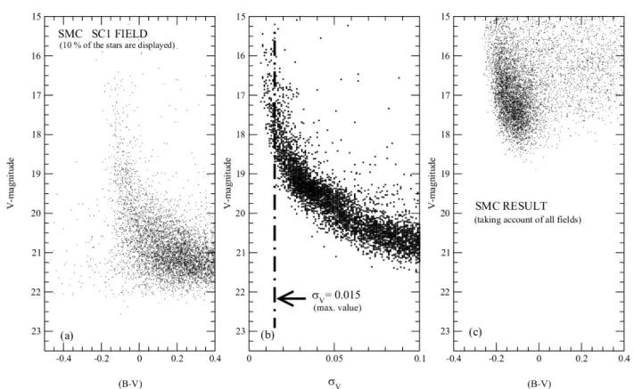
Fig. 1. a)CM-Diagram for the OGLE 2 SC 1 field, 10% of the data have been plotted for sake of clarity. b) Standard deviation of the measure-ments: σV versus magnitude V, the dot-dashed line indicates the limit-value considered (0.015). c) The resulting CM-diagram after selection
(all the fields within SMC have been plotted).
The question of a metallicity dependence must also be ad-dressed. Ribas et al. (2000)’s results suggest a slight metallic-ity dependence for a stellar mass around 2.40 M (see their Table 1). The more metal poor star SZ Cen (in mass frac-tion: Z0 = 0.007) is satisfactorily modelled with an
over-shooting distance 0.1 Hp <∼ lov <∼ 0.2 HP and objects with
Z0 ranging between 0.015 and 0.020 seem to have an
over-shooting around 0.2 HP. Keller et al. (2001) have recently
explored the dependence of overshooting with metallicity by means of the isochrone technique using isochrone grids from the Padova group. Their study involves HST observations of four clusters: NGC 330 (SMC), 1818, 2004 and 2001 (LMC). Keller et al. (2001) find the best fit (with respect to age and overshooting) for an overshooting amount which is equivalent to lover = 0.31 ± 0.11 Hp in the Geneva formalism (lPadovaover =
2× lGeneva over ).
In this paper, we carry out an independent study of a possi-ble metallicity dependence of overshooting with a technique which differs from the “binary system” (Ribas et al. 2000; Andersen 1991) and “isochrone” techniques. Our method is based on star-count ratios, with comparisons between obser-vational material and synthetic population results in color-magnitude (CMD) diagrams. We are then led to discuss several points: particularly distance modulus, reddening and binarity rate. If the dependence of overshooting on metallicity (or mass) was thereby to be firmly assessed, it would then be a challenge to understand its physical origin.
We are concerned with a metallicity range relevant to the Magellanic Clouds and take advantage of the homogeneous
OGLE 2 data, which provide color magnitude diagrams for ∼2 × 10⁶stars in the Small Magellanic Cloud (hereafter SMC)
and∼7 × 10⁶in the Large Magellanic Cloud (hereafter LMC).
On the theoretical side, we estimate the number of stars from evolutionary model sequences computed with different amounts of overshooting. From these data sets and using evo-lutionary models with intermediate and low metallicity, we es-timate the overshooting value during the main sequence in the SMC and LMC for a stellar mass in the range 2.5 M –25 M .
In Sect. 2 we describe the observational data involved in this work. Section 3 is devoted to the method used: data se-lection and star counting. Section 4 gives the main features of our population synthesis procedure. Section 5 is devoted to as-trophysical inputs, and Sect. 6 to results and effects of uncer-tainties. Section 7 discusses the results. It must be emphasized that we determine in fact the extent of the inner mixed core re-gion which can be due either to true overshooting or to another process such as rotation; some observational evidence exists about correlation between metallicity and v sin i (see Venn et al. 1999). The problem of rotation is briefly discussed in Sect. 7. Finally, Sect. 8 gives some comments and concluding remarks. An appendix has been added to provide details about the pop-ulation synthesis algorithm and error simpop-ulations.
2. Observational data
The observational data set considered here has been obtained by the Optical Gravitational Lensing Experiment (OGLE hereafter) consortium during its second operating phase
(for more details and references the reader can consult URL: http://www.astrouw.edu.pl/ogle/).
2.1. SMC and LMC data
We have downloaded the SMC data described in Udalski et al. (1998). The data used in this paper are from the post-Apr. 8, 2000 revision. The SMC is divided into 11 fields (labeled SC1 to SC11) covering 550× 140; each field contains between ∼100 000 and ∼350 000 objects. For each object several quanti-ties are available: equatorial coordinates, BV I photometry and associated standard errors σB, σV and σI. This database has the
great advantage of being extensive and very homogeneous. The LMC data are described in Udalski et al. (2000). The BV I map of the LMC is composed of 26 fields (SC1 to SC26) in the central bar of the LMC. The dataset includes photometry and astrometry for about 7 million stars over a 5.7 square degree field.
3. The star-count method
3.1. Data selection
As shown in Fig. 1b, the standard error on V-magnitude, σV,
increases with the magnitude. This is also true for B or I-magnitudes. Hence the errors on (B− V) or (V − I) colors rapidly increase and reach values as large as 0.2 mag around a V-mag∼ 20: this is of the same order as the Main Sequence width.
As we are interested in the MS structure and as we must minimize error effects while keeping quite good statistics, we have chosen to take into account only data with σV and σB
(or σI) lower or equal to 0.015 mag, leading to a maximum
er-ror on color of 0.02 mag. The value of 0.015 mag appears to be an optimal choice maintaining a good statistics with photo-metric errors remaining small compared with the MS width. Figure 1 sketches the proposed selection process and dis-plays differences between the entire Color-Magnitude Diagram (Fig. 1a) and the final diagram (Fig. 1c): obviously, the remain-ing data are those correspondremain-ing to lower magnitudes.
This selection process leaves ∼4700 objects on the SMC MS (over a total of more than 2.2 millions objects) in the BV system (∼1100 objects in the VI system) and ∼4000 ob-jects on the LMC MS (over a total of more than 7.2 millions objects) in the BV system (∼1600 objects in the VI system). As we can see, the BV system presents more favorable statis-tics, therefore in the following we will work only with this set of bands.
Tables 4 from Udalski et al. (1998, Udalski et al. 2000) in-dicate that completeness for V <∼ 18 should be better than about 99% for the SMC; and should be around 96%−99% depending on the field crowding for the LMC.
3.2. Star count ratios: An observational constraint As the absolute number of stars arriving on the ZAMS per unit of time for a given mass is unknown, we rather com-pute star count ratios. To count stars, we first define an area
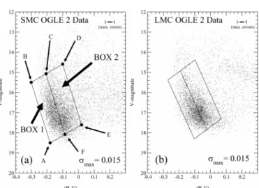
Fig. 2. a)Data from SMC with σV ≤ 0.015 mag and box definitions
(N1 + N2 = 4653 and N2/N1 = 1.08), b) the same for the LMC
case (N1+ N2= 4113 and N2/N1= 1.01).
in the CM-diagram. As we are interested in the MS structure, we choose a region which contains the main sequence “bulge” revealed after the data selection process (see Fig. 2a) with the most convenient geometrical shape: a “parallelogram” (for au-tomatic count purpose). A couple of opposite sides (AB and DE in Fig. 2a) are chosen to be more or less “parallel” to the main sequence axis.
In the CM-Diagram, main sequence stars evolve from the blue to the red side. The MS width is mainly an evolutionary effect connected to a characteristic time scale τMS (time spent
by a star on the Main Sequence). The distribution of the objects within the Main Sequence should be related to this time scale. Therefore we divide our parallelogram into two regions called “box 1” and “box 2” (see Fig. 2a) where the respective numbers of objects N1 and N2 are similar (N2/N1 ∼ 1). This ratio is
taken as an observational constraint and it will enable us to discriminate between theoretical grids of evolutionary tracks computed with various overshooting amounts.
We now turn to the method used to build a synthetic stellar sample comparable to the OGLE 2 ones (after selection) from evolution simulation outputs.
4. Population synthesis
4.1. Evolutionary models
Our evolutionary models are built with the 1D Henyey type code CESAM1(see Morel 1997) in which we brought several improvements. Applying modern techniques like the projection of the solutions on B-spline basis and automatic mesh refine-ments, CESAM allows robust, stable and highly accurate cal-culations. We use as physical inputs:
– the OPAL 96 opacities from Iglesias & Rogers (1996) at high temperatures (T > 10 000 K) and the Alexander & Ferguson (1994) opacities for cooler domains. For metallic-ity higher than the solar one (that occurs during the He core 1 CESAM: Code d’ ´Evolution Stellaire Adaptatif et Modulaire.
burning phase) we use elemental opacities (Los Alamos) calculated by Magee et al. (1995);
– the EFF equation of state from Eggleton et al. (1973); – elemental abundances are from Grevesse & Noels (1993)
(the “GN93” mixture), the cosmological helium is from Izotov et al. (1997): YP = 0.243, and the helium content
is scaled on the solar one following a standard helium-metallicity relation: Y = YP+ Z(∆Y/∆Z). The calibration
of a solar model in luminosity yields∆Y/∆Z = 2 (Lebreton et al. 1999) from the calibration of the solar model radius. This value is compatible with the recent value∆Y/∆Z = 2.17± 0.40 of Peimbert et al. (2000). We therefore adopt ∆Y/∆Z ≈ 2;
– for the chemical composition we adopt [Fe/H] derived from Cepheid measurements by Luck et al. (1998):
– for the SMC they find a range from−0.84 to −0.65 with a mean value: [Fe/H] = −0.68 which leads to X0 =
0.745, Y0= 0.251 and Z0= 0.004.
– for the LMC they find a range from −0.55 to −0.19, combining all the values we obtain a mean value of [Fe/H] = −0.34 leading to: X0 = 0.733, Y0 = 0.259
and Z0= 0.008;
– The nuclear reaction rates are from Caughlan & Fowler (1988), except: 12C(α, γ)16O, 17O(p, γ)18F taken from
Caughlan et al. (1985) and17O(p, α)14N taken from Landr´e
et al. (1990). The adopted rate for12C(α, γ)16O is quite
sim-ilar to the NACRE compilation (Angulo et al. 1999) one: a factor of about two higher than Caughlan & Fowler (1988) and about 80% of Caughlan et al.’s (1985) one.
– To take into account the metallicity effect on the mass loss rate (de Jager et al. 1988) we adopt the scaling factor (Z0/0.02)0.5derived from the Kudritzki & Hummer (1986)
models;
– The convective flux is computed according to the classi-cal MLT. We use a mixing length value lMLT = 1.6 HP.
This value has been derived by Schaller et al. (1992) from the average location of the red giant branch of more than 75 clusters. A very similar value (1.64) has been found more recently by Lebreton et al. (1999). An extra-mixing zone is added above the Schwarzschild convective core: this “extra-mixing” zone is set to extend over the distance
lover = αover HP, αover being a free parameter, the value of
which is discussed here;
– the external boundary conditions are determined in a layer within a simple grey model atmosphere built with an Eddington’s T (τ) law.
4.2. Conversion of the theoretical quantities into observational ones
In order to compare theoretical results to observational data, conversions are needed. Transformations of the theoretical quantities, (Mbol, Teff) into absolute magnitudes and colors
are derived from the most recent version of the Basel Stellar Library (BaSeL, version 2.2), available electronically at ftp://tangerine.astro.mat.uc.pt/pub/BaSeL/. This library provides color-calibrated theoretical flux distributions
for a large range of fundamental stellar parameters, Teff (2000
to 50 000 K), log g (−1.0 to 5.5 dex), and [Fe/H] (−5.0 to +1.0 dex). The BaSeL flux distributions are calibrated on the stellar U BVRI JHKL colors, using:
– empiricalphotometric calibrations for solar metallicity; – semi-empiricalrelations constructed from the color
differ-ences predicted by stellar model atmospheres for non-solar metallicities.
Details about the calibration procedure are given in Lejeune et al. (1997) and Lejeune et al. (1998). Compared to the previ-ous versions of the BaSeL library, all the model spectra of stars with Teff ≥ 10 000 K are now calibrated on empirical colors
from the Teff versus (B− V) relation of Flower (1996). In
ad-dition, the calibration procedure for the cool giant model spec-tra has been extended in the present models to the parameter ranges 2500 K≤ Teff < 6000 K and −1.0 ≤ log g < 3.52.
4.3. Population synthesis
In contrast with “classical” works on population synthesis where the CMD as a whole is simulated, we construct a small part of the CMD: the area containing the brighter MS stars. In this way the task is simplified. Artificial stellar samples have been generated from our evolutionary tracks with a specially designed population synthesis code CReSyPS3.
In our framework the main hypothesis is that the Star Formation Rate (SFR) is constant during the time scales in-volved here: i.e. a few hundred megayears. So for a given mass the number of observed stars (i.e. those corresponding to a given evolutionary track) must be proportional to the time scale of the main sequence. We assume that the SFR is constant in time and mass (equal for all masses in the range explored in this work), if we note r the SFR:∆t ≈ 1/r represents the mean time elapsed between two consecutive star births. For the observa-tional star samples,∆t is unknown but the objects numbers are available. We choose ∆t to get similar total star numbers in boxes 1 and 2 (i.e. N1+ N2) both in the synthetic CMD and
observational diagram. We point out that the ratios N2/N1 are
not sensitive to the∆t value chosen.
The evolutionary track grids scan a mass range between 2.5 M and 25 M from the ZAMS to log Teff ∼ 3.8
cover-ing the entire box ranges in color and magnitude (defined in Sect. 3.2). The mass step is increasing from 0.5 M around 3 M stars to 5 M above 15 M . Several overshooting amounts have been used from 0.0 to 0.8. CReSyPS treats the photomet-ric errors by simulating OGLE 2 ones (see Appendix A) which is very important for our purposes. Our algorithm requires the knowledge of some input parameters: distance modulus, reddening and absorption, binarity rate, Initial Mass Function (hereafter IMF) slope and photometric errors.
2 In the previous versions of the BaSeL models, we adopted T eff=
5000 K and log g= 2.5 as the upper limits for the calibration of giants (see Lejeune et al. 1998).
We summarize here the main steps of the algorithm: – STEP 1:a mass distribution is generated between 2.5 M
and 25 M following the Salpeter’s law: dN/dm≈ m−αSalp (see Sect. 5.4).
– STEP 2:for each mass, an evolutionary track is interpo-lated within the grid calcuinterpo-lated by the evolutionary code. On each track, models are selected every time step ∆t, which is adjusted in order to yield a total number of stars equivalent to the observed one.
– STEP 3: consistently with the value of the binary rate < β > (see Sect. 5.3), objects are randomly selected to belong to a binary system and the magnitudes of these sys-tems are calculated. Triple syssys-tems (and higher multiplicity systems) are neglected.
– STEP 4: distance modulus is added (and in the case of SMC a random “depth” inside the cloud) and syn-thetic photometric errors are attributed to magnitudes (see Appendix A).
– STEP 5: we use a “quality filter”: objects with too large photometric errors are rejected from the synthetic sample. – STEP 6:color is calculated, reddening and extinction
coef-ficient are applied. Concerning reddening, a gaussian distri-bution is applied around the mean value in order to simulate object-to-object variations (see discussion in Sect. 5.2). With the interpolation between evolutionary tracks, it is very important (particularly at low mass, i.e. 3.0 M <∼ M <∼ 4.0 M ) to reproduce the time scale τMSwith a good accuracy. A test at
3.25 M has shown that the “interpolated time scale”, τinterpolMS , is very close to the calculated one (with the evolutionary code) τcal
MS with a difference not larger than about 1%. Also
impor-tant are the magnitude interpolations on the Main Sequence: our tests also show a very good agreement between interpo-lated magnitudes and calcuinterpo-lated ones, differences are unsignif-icant (about 10−3−10−2 mag, whereas the photometric errors are much larger).
Our code intensively uses a random number generator. We have chosen an algorithm insuring a very large period about 2× 10¹⁸ (program “ran2” from Press et al. 1992), which is much larger than the number of synthetized objects.
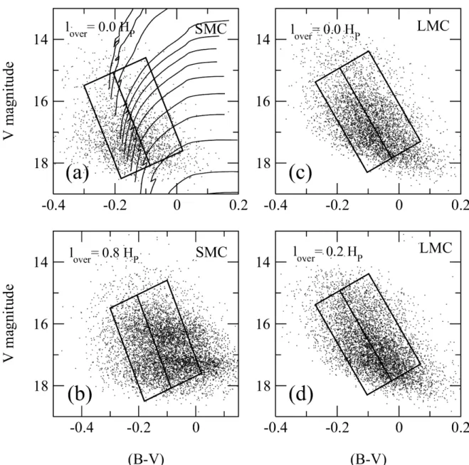
As a result, examples of synthetic samples generated by CReSyPSare displayed in Fig. 3 where the influence of over-shooting is shown for both clouds.
5. Astrophysical inputs
5.1. Distance modulus
Large Magellanic Cloud. The LMC distance modulus has a key role in extragalactical distance determinations, but its value is still debated. The determinations range between “short” dis-tance scales (i.e. Stanek et al. 1998) and “long” disdis-tance scales (i.e. Laney & Stobie 1994). Using the HIPPARCOS calibrated red clump stars, Stanek et al. (1998) found µ0, LMC= 18.065 ±
0.031± 0.09 mag and Laney & Stobie (1994) from a study of Cepheids Period-Luminosity relation obtained µ0, LMC =
18.53 mag with an internal error of 0.04 mag. Groenewegen & Salaris (2001) found µ0, HV 2274 = 18.46 ± 0.06 mag from a
study of the LMC-eclipsing binary system HV 2274. They in-dicate a LMC center distance at µ0, LMC = 18.42 ± 0.07 mag.
Recently, from the DENIS survey data, Cioni et al. (2000) de-rived a distance modulus for the LMC of µ0, LMC= 18.55±0.04
(formal)±0.08 (systematic) using a method based on the appar-ent magnitude of the tip of the red giant branch. The HST Key Project Team adopted µ0, LMC= 18.50±0.15 mag (Mould et al.
2000). In order to bracket the most recent estimations, we have chosen the HST Key Project value:
µLMC= 18.50 ± 0.15 mag.
Van der Marel & Cioni (2001) give an order of magnitude of the depth of the LMC. They indicate small corrections to magni-tude for well studied individual objects within the LMC, rang-ing between∆µ0, LMC = −0.013 (SN 1987A) to ∆µ0, LMC =
+0.015 (HV 2274). We neglect these corrections which have the same order of magnitude than the photometric errors. Small Magellanic Cloud. Laney & Stobie (1994) suggest a distance modulus (based on Cepheids) of µ0, LMC= 18.94 mag
with an internal error of 0.04 mag; this modulus decreases by about 0.04 mag if calibrators are half-weighted. More re-cently Kov´acs (2000) (with a method based on double mode Cepheids), find µ0, LMC = 19.05 ± 0.13 mag and Cioni et al.
(2000) have µ0, LMC = 18.99 ± 0.03 (formal) ±0.08
(system-atic) mag. We retain the following estimation: µSMC= 18.99 ± 0.10 mag.
The SMC distance modulus only represents an average dis-tance. Crowl et al. (2001) have evaluated the depth of the SMC along the line-of-sight by a study of populous clusters. They derived a depth between ∼6 kpc and ∼12 kpc; these values lead to magnitude differences of 0.2 and 0.4 mag respectively. Previous studies, see for instance Gardiner et al. (1991), show similar results with a line-of-sight SMC depth ranging between ∼4−7 kpc and ∼15 kpc strongly depending on the location in the SMC.
We have chosen to model the SMC depth with a gaussian distribution of distances around µSMCwith a standard deviation:
σdepth
SMC = 0.05 mag
which represents a total depth of∼8 kpc (about ∼0.3 mag). 5.2. Reddening and absorption
We have to distinguish: foreground reddening E(B− V)MW
(due to material in Milky Way) and internal redden-ing E(B− V)i with an origin into the Cloud itself.
These quantities are expected to change along the line-of-sight. Here we model the total reddening as
E(B− V)MW+i= E(B − V)MW+ E(B − V)itaking into account
its non-uniformity. From the literature, we derive estimations for the mean value and the dispersion of E(B− V)MW+i,
object-to-object variations can then be simulated.
We now discuss reddening determinations for the SMC and LMC. From a study of spectral properties of galactic nuclei be-hind the Magellanic Clouds, Dutra et al. (2001) have evaluated the foreground and background reddenings for both Clouds.
Fig. 3.Synthetic CM-Diagrams for SMC and LMC chemical compositions, panels a) and b) are for the SMC with two overshooting amounts: αover= 0.0 and αover= 0.8, panels c) and d) are for the LMC with: αover= 0.0 and αover= 0.2 respectively. For panel a) only 30% of the synthetic
objects have been displayed for clarity purpose and corresponding evolutionary tracks have been plotted. For other panels: b)–d) the number of displayed objects has not be reduced. In all cases the total number of stars in the boxes -used for calculations- is close to the observational one: a) N1+ N2= 4403 (N2/N1= 0.65), b) N1+ N2= 5011 (N2/N1= 1.59), c) N1+ N2= 3582 (N2/N1= 0.94), d) N1+ N2= 4717 (N2/N1= 1.13).
We recall that empirically we got for the SMC N1+ N2 = 4653 (N2/N1 = 1.08) and for the LMC N1+ N2 = 4113 (N2/N1 = 1.01). The ratios
N2/N1obtained theoretically are rather independant from the value of N1+ N2in the synthetic CM-Diagram, for instance in the case of the
panel b) we got N2/N1 = 1.60 with N1+ N2 = 6399. The cloud of dots in panel b) (lover= 0.8 Hp, SMC) calls a comment: it appears to be
bimodal, i.e. showing over-populated regions around V∼ 17.5 mag and V ∼ 16.3 mag. Indeed for high overshooting values the main sequence of masses as small as∼3 M can reach V ∼ 17.5 generating with their large evolutionary time scale an over-populated region. Moreover the binarity shifts a part of this population to a∼0.8 mag brighter region, with a binarity rate β = 0.0, this “bimodal effect” disappears.
For the LMC, they found an average spectroscopic reddening of E(B− V)MW+i= 0.12 ± 0.10 mag. The uncertainties
essen-tially come from the determination of the stellar populations belonging to background galaxies: in the case of LMC, when Dutra et al. (2001) consider only red population galaxies, they find E(B− V)MW+i= 0.15 ± 0.11 mag, which gives an idea of
the global uncertainty on E(B− V), which should be around ∼0.02−0.03 mag (about ∼13−20%). For the SMC Dutra et al. (2001) find E(B− V)MW+i= 0.05 ± 0.05 mag. The OGLE 2
project provides reddening for each Cepheid star discovered in both Clouds. OGLE values are: E(B− V)MW+i= 0.09 ± 0.01
(SMC) and E(B− V)MW+i= 0.15 ± 0.02 (LMC). In Fig. 4 we
have displayed the histogram of E(B− V)MW+i values from
Dutra et al. (2001) and OGLE group. OGLE data have a better statistics with respectively 1333 (SMC) and 2049 (LMC) ob-jects, against 14 (SMC) and 22 (LMC) for Dutra et al. (2001). Dutra et al’s data are systematically less red; this could be in-herent to their method: they observed objects behind Clouds
and observations are easier through the more transparent re-gions of the clouds.
In addition, Oestreicher et al. (1995) have determined the reddening for 1503 LMC foreground stars with a U BV photom-etry based method: E(B− V)MW= 0.06 ± 0.02 mag, a quite
low value because it is related to foreground stars. It shows a spread (0.02) similar to the OGLE 2 one. Oestreicher et al.’s (1995) distribution is in very good agreement (see Fig. 4b) with Dutra et al.’s one, which tends to confirm that Dutra et al.’s re-sult could be underestimated (Dutra et al.’s rere-sults are supposed to take account foreground and internal reddeing). Therefore in the case of LMC, we prefer to retain the OGLE average value for purpose of consistency:
h E(B − V)LMC
MW+ii = 0.15 mag.
Figure 4b shows that the distribution shape is the same for Dutra et al. (2001) and Oestreicher et al. (1995), the OGLE one being quite narrow which appears slightly underestimated, thus we take a value similar to Dutra et al. one:
σLMC
E(B−V)MW+i = 0.08 mag.
We take into account an additional uncertainty on h E(B − V)LMC
MW+ii of about:
δLMC
E(B−V)= 0.02 mag.
The SMC case is more questionable (we only have two sets of data), we favor the OGLE values because they are likely more suitable for performing simulations which synthesize OGLE data. Moreover OGLE data have larger statistics. We adopt: h E(B − V)SMC
MW+ii = 0.09 mag
with a crudely estimated uncertainty of about: δSMC
E(B−V)= 0.015 mag.
In this case also, the OGLE standard deviation (see Fig. 4a) seems to be low, therefore we adopt the Dutra et al. (2001) one:
σSMC
E(B−V)MW+i = 0.05 mag.
The absorption coefficient is taken from Schlegel et al. (1998):
AV = 3.24 × E(B − V)MW+i
and is calculated for each object. 5.3. Binary rate
Evaluating the average binary rate < β > in objects as extended as the Magellanic Clouds is not easy. Locally (i.e. within a par-ticular area of the galaxy) this multiplicity rate depends – at least – on two factors: (1) the star density and the kinemat-ics of the objects which influence the encounter probability; (2) the initial binary rate (relative number of binaries on the ZAMS). Within the Magellanic Clouds, the binary rate likely varies over a wide range and we only consider its spatial aver-age value < β >. 0 0.02 0.04 0.06 0.08 0.1 0.12 0.14 E(B-V) 0 0.1 0.2 0.3 0.4 0.5 0 0.1 0.2 E(B-V) 0 0.05 0.1 0.15 0.2 0.25 SMC Data LMC Data (a) (b)
Fig. 4. Relative number of stars Nstars/Ntot versus reddening from
Dutra et al. (2001) (dashed curve), OGLE 2 experiment Cepheid catalogue: see Udalski et al. (1999) and Udalski et al. (1999), and data read in Fig. 24 of Oestreicher et al. (1995) (dot-dashed curve). a)Data for SMC, b) data for LMC.
Ghez (1995) finds in the solar neighbourhood that for main sequence stars and young stars the binary rate < β > ranges between 0.10 and 0.50 (it peaks at < β >= 0.50). Therefore we tested the effects of binarity for these two extreme values.
In our population synthesis code, binaries are taken into ac-count with a uniform probability for the mass ratio q= M2/M1
(in the considered mass range).
5.4. IMF slope
The IMF has been extensively discussed by many authors. Toward both Galactic poles and within a distance of 5.2 pc from the Sun, Kroupa et al. (1993) found a mass function: dN/dm≈ m−αSalp with α
Salp≈ 2.7 for stars more massive than
1 M . In the LMC, Holtzman et al. (1997) inferred – from HST observations – a value consistent with the Salpeter (1955) one: αSalp≈ 2.35. At very low metallicity, Grillmair et al. (1998)
ob-served the Draco Dwarf spheroidal Galaxy ([Fe/H]≈ −2) with the HST. They concluded that the Salpeter IMF slope remains valid in the Magellanic Clouds and we have chosen:
αSalp= 2.30 ± 0.30.
However we must keep in mind that some circularity in work exists when using an IMF. As described by Garcia & Mermilliod (2001) the IMF can be derived from the observed Present Day Mass Function (PDMF) using evolutionary tracks and their corresponding time scales which depend on the adopted value for the overshooting!
5.5. Star formation rate
For a given mass, the Star Formation Rate (SFR) represents the number of stars “created” per unit of time. Vallenari et al. (1996) have studied three stellar fields of the LMC and have found a time scale of about∼2–∼4 Gyr for the “bulk of star formation”. We therefore make the reasonable assumption that the SFR remained quite constant during the short galactic pe-riod relevant for this work, i.e. for the last∼300 Myr. The SFR involved here is an average value over each cloud.
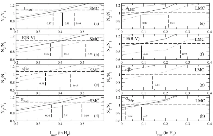
6. Resulting overshooting amounts
6.1. Large Magellanic Cloud
As a first step we choose the mean values for each astrophys-ical input (discussed in Sect. 5), this yields for the LMC the following overshooting:
lover= 0.09 Hp
which is a rather mild amount. We examine in Fig. 5 how the
lover-value is affected by the uncertainties on the astrophysical
inputs:
– Changing the IMF slope αSalpin the range 2.0−2.6 we
ob-tain:
0.02 <∼ lSalpover <∼ 0.09 Hp
which tends to minimize the overshooting.
– Next, a test with the average binary rate < β > in the range 0.10− 0.50 leads to:
0.00 <∼ l<β>over <∼ 0.14 Hp.
– A distance modulus value in the range 18.35 <∼ µLMC <∼
18.65 enables us to derive: lover = 0.0 Hp (in fact for
µLMC= 18.35 all the values for simulated N2/N1are larger
than the observed one) and lover = 0.21 Hp for µLMC =
18.65.
– An average reddening between 0.13 and 0.17 leads respec-tively to lover = 0.0 Hp (in this case also all the values
for simulated N2/N1are larger than the observed one) and
lover= 0.27 Hp.
We stress that uncertainties on distance modulus and reddening infer the largest uncertainties on the final overshooting values. We retain for the LMC average chemical composition:
lLMCover = 0.10+0.17−0.10Hp
which indicates that a mild overshooting amount around ∼0.1−0.2 Hp is needed to model LMC stars as found in the majority of determinations involving solar chemical composi-tion objects (see Sect. 1).
6.2. Small Magellanic Cloud
For the SMC, using the mean value of each astrophysical inputs we obtain (see also Fig. 5):
lover= 0.41 Hp.
– If the IMF slope varies between extreme values (−2.0 <∼ αSalp<∼ −2.6), the overshooting varies within the following
boundaries:
0.36 <∼ lIMFover <∼ 0.50 Hp
similarly, an average binary rate ranging between 0.10 and 0.50 leads to:
0.34 <∼ l<β>over <∼ 0.45 Hp.
– The uncertainty on SMC distance modulus (18.89 <∼ µSMC<∼ 19.09) leads to:
0.37 <∼ lµover <∼ 0.46 Hp.
– Similarly if one considers the uncertainty on the aver-age reddening (< E(B− V) > ranging between 0.075 and 0.105), the overshooting amount shows a high sensitivity to reddening:
0.36 <∼ lE(Bover−V) <∼ 0.52 Hp.
Again, uncertainties on distance modulus and reddening are the largest. We retain for the SMC:
lSMCover = 0.40+0.12−0.04Hp.
Whatever the simulation is, statistical errors are of the order of 0.01 Hp which can be safely neglected. In the SMC case, the required overshooting appears to be much larger than for LMC stars and for solar composition stars.
7. Discussion
7.1. An upper limit with Roxburgh’s criterion
Roxburgh’s criterion (Roxburgh 1989) is a very general con-straint on the size of the convective core. It is written as an integral formulation over the stellar core radius:
Z r=Rcore r=0 (Lrad− Lnuc) 1 T2 dT drdr= Z r=Rcore r=0 Φ T4πr 2 dr (1)
where Lrad and Lnuc are respectively the radiative energy flux
and the total energy flux (in J s−1) generated by nuclear pro-cesses, r is the radius, Rcore is the core size including the
“overshooting” region. Φ represents the viscous dissipation (in J s−1m−3). In the whole stellar convective core the turbu-lence is supposed to be statistically stationary and the tempera-ture gradient has to be almost adiabatic. In Eq. (1) the integrand is positive when r is lower than the Schwarzschild boundary where Lrad= Lnucand it becomes negative beyond.
The viscous dissipationΦ is unknown but the integral con-straint is satisfied for larger Rcore value whenΦ = 0. Hence,
neglecting the dissipation by settingΦ = 0 provides the maxi-mum possible extent of the convective core which can be con-sidered as the upper limit for overshooting. Evolutionary tracks have been calculated, using Roxburgh’s criterion, for a repre-sentative mass of 6 M and SMC and LMC metallicities. The equivalent overshooting amount (EOA), given in Table 1, is the time weighted average overshooting distance along the evo-lutionary tracks, expressed in pressure scale height.
0.2 0.3 0.4 0.5 0.6 0.8 1 1.2 N 2 /N 1 0 0.1 0.2 0.3 0.4 0.6 0.8 1 1.2 N 2 /N 1 0.2 0.3 0.4 0.5 0.6 0.8 1 1.2 N 2 /N 1 0 0.1 0.2 0.3 0.4 0.6 0.8 1 1.2 N 2 /N 1 0.2 0.3 0.4 0.5 0.6 0.8 1 1.2 N 2 /N 1 0 0.1 0.2 0.3 0.4 0.6 0.8 1 1.2 N 2 /N 1 0.2 0.3 0.4 0.5 lover (in HP) 0.6 0.8 1 1.2 N 2 /N 1 0 0.1 0.2 0.3 0.4 lover (in HP) 0.6 0.8 1 1.2 N 2 /N 1 µSMC µLMC E(B-V) E(B-V) <β> <β> αSalp αSalp SMC SMC SMC SMC (a) (b) (c) (d) (e) (f) (g) (h) LMC LMC LMC 0.41 LMC 0.41 0.41 0.46 0.37 0.36 0.52 0.45 0.36 0.50 0.09 0.09 0.09 0.21 0.27 0.14 0.02 0.34
Fig. 5.Overshooting determinations for SMC (panels a–d)) and LMC (panels e–h)). The influence of distance modulus, reddening and IMF slope are considered for each cloud: continuous lines correspond to central values of these parameters discussed in Sect. 5 and dashed lines to the associated error bars. Inferred values of lover(and uncertainties) are given on each figure. For c) and g) panels, dotted line is for < β >= 0.0
and dot-dashed for < β >= 0.5 (see text).
Table 1.Time weighted average overshooting distances for a 6 M main sequence model, derived with the “Roxburgh’s criterion” ne-glecting dissipative phenomenon (Φ = 0).
Metallicity Z0 0.004 (SMC) 0.008 (LMC)
Average EOA 0.6 Hp 0.6 Hp
In both cases (LMC and SMC), Roxburgh’s criterion pre-dicts a maximum value (i.e. neglecting viscous dissipation) around 0.6 Hp (see Table 1) independent from Z0. Our
deter-minations – i.e. lSMC
over = 0.40+0.12−0.06Hp and lLMCover = 0.10+0.17−0.10
Hp-therefore are compatible with the theoretical upper limit given by the Roxburgh’s criterion.
7.2. Influence of rotation
In addition to convection, rotation is an other important phe-nomenon inducing mixing through shear effects and other in-stabilities. For instance Venn (1999) finds surface abundance variations in SMC A supergiants that could be explained by some kind of mixing related to rotation.
Taking account of the rotational effect brings new impor-tant unknown features: (1) theΩ-value distribution and (2) the v sin i distribution for the considered stellar population. Both features remain unconstrained by observational studies.
In addition, stellar rotation involves many effects and phys-ical processes that are non-trivial to include in modern evolu-tionary codes. Talon et al. (1997) show that (see their Fig. 5) a rotating 1D-model with an initial surface velocity of 300 km s−1 leads to a main sequence track equivalent to an overshooting model using lover = 0.2 Hp. Despite great theoretical efforts, a
free parameter remains for horizontal diffusivity in Talon et al. (1997) treatment of rotational mixing (see Zahn 1992).
Rotation changes the global shape of an evolutionary track, through two distinct effects: (1) the material mixing inside the inner part of the star which brings more fuel into the nu-clear burning zones like overshooting, (2) the effective surface gravity modification leading to color and magnitude changes (which depend on the angle between the line-of-sight and the rotational axis). In their Fig. 6, Maeder & Meynet (2001) show the influence of rotation on evolutionary tracks for low metal-licity objects (Z0 = 0.004). These tracks have been calculated
taking into account: (1) an “average effect” on surface, (2) the internal mixing. These tracks are very similar to those calcu-lated with different overshooting amounts values.
An additional effect which needs to be discussed here is the surface effect: modifications of colors and magnitudes of MS stars due to rotation (in absence of any mixing phe-nomenon) have been studied by Maeder & Peytremann (1970) with uniformly rotating models. Their Table 2 gives expected changes of MVand (B− V) as a function of Ω (angular velocity
0 100 200 300 400
v sin i (km.s-1)
0 0.1 0.2
Rel. Numb. of Objects
Data from Wolff & Simon (1997)
(15 < mV < 18.5)
Fig. 6.Relative number of stars (Nstars/Ntotversus V× sin i for Wolff
& Simon (1997) objects with magnitudes in our studied range.
expressed in break-up velocity unit) and v sin i (this latter ranges from 0 to 457 km s−1, for a 5 M star). In this table standard deviation for MV and (B− V), are: σMV = 0.18 mag and σ(B−V) = 0.01 mag. Therefore the rotation effect has
roughly the same order of magnitude than present uncertainties on magnitudes and colors. However, stars with v sin i greater than ∼200 km s−1 are quite rare, as shown by the data of Wolff & Simon (1997) (see Fig. 6). Then keeping only data with v sin i <∼ 200 km s−1, leads to: σMV = 0.20 mag and σ(B−V)= 0.001 mag. The effect on absolute magnitude remains
of the same order, whereas the effect on color becomes largely negligible. We conclude that our results remain valid, even if the major mixing is due to rotation. In this case, the value of
loverwould change its meaning. Major contribution to lovervalue
would represent a shear effect mixing.
7.3. Influence of chemical composition gradient We have sofar assumed a uniform chemical composition. The chemical composition may vary inside each Magellanic Cloud. The existence of an abundance gradient in the Clouds is still debated and spectroscopic measurements with a statistics as large as the statistics of OGLE 2 data are not available. In their Table 4, Luck et al. (1998) give spectroscopic determinations of [Fe/H] for 7 SMC Cepheids and 10 LMC Cepheids. For SMC data, the standard deviation is σSMC
[Fe/H] ∼ 0.07 dex leading to
negligible variations for the heavy elements mass fraction Z0.
Therefore the SMC can be considered as chemically homoge-neous for our purpose. For LMC, Luck et al. (1998) find a stan-dard deviation σLMC[Fe/H] ∼ 0.10 dex giving 0.007 <∼ Z0 <∼ 0.01.
From evolutionary tracks of typical mass (6 M ) and an over-shooting of 0.1 HP, changing Z0from 0.007 to 0.01 has a
negli-gible effect on magnitude and an effect of ∼0.003 mag on color, which is largely lower than the photometric errors. We con-clude that – in the light of the present knowledge – the chemical composition gradient does not change our results significantly. 7.4. Comparison with other works
From the investigation of young clusters in the Magellanic Clouds, Keller et al. (2001) did not find any noticeable over-shooting dependence with metallicity. They obtained for NGC 330 (Z0 ∼ 0.003) lNGC 330over = 0.34 ± 0.10 Hp, which is
compatible with our determination for the SMC: lSMC over =
0.40+0.12−0.04Hp. For NGC 2004 (Z0 ∼ 0.007) Keller et al. (2001)
0 0.01 0.02 0.03 Z0 0 0.1 0.2 0.3 0.4 0.5 l over (in H P )
Fig. 7.Overshooting parameter αoverversus metallicity Z0 from
vari-ous sources. Open triangles represent results from Ribas et al. (2000) for SZ Cen (Z0 ∼ 0.007) error bars have been indicated, arrows
mean that the derived value is a minimum. The open square shows a result from Kozhurina-Platais et al. (1997) for the galactic cluster NGC 3680, error bars are indicated. Filled triangles are determinations from Keller et al. (2001): with continuous error bars amounts corre-sponding to the SMC cluster NGC 330, NGC 1818, NGC 2100 and with dashed error bars result for the LMC cluster NGC 2004. Open circle: determination in Hyades cluster from Lebreton et al. (2001) (upper limit for overshooting). Filled diamonds: SMC and LMC de-terminations performed in this work. Errors on Z have been evaluated assuming an internal error on [Fe/H] of 0.1 dex.
got lNGC 2004
over = 0.31 ± 0.11 Hp; while for similar metallicity
we derived lLMC
over = 0.10+0.17−0.10Hp which is also compatible with
Keller et al.’s result. One can note that masses involved in our simulations (average mass of∼7−8 M with a standard devia-tion of 4 M ) are higher than the Keller et al. (2001) one (termi-nus masses in the range 9−12 M for the four clusters). Keller et al. (2001) do not discuss the influence of the uncertainty on distance modulus of the clusters and use µLMC = 18.45 mag
and µSMC= 18.85 mag.
Ribas et al. (2000) derive overshooting amounts from evo-lutionary models of galactic binary systems. For SZ Cen (Z0 ∼
0.007) they find 0.1 <∼ lover <∼ 0.2 Hp which is close to our
value for the LMC, but the mass of SZ Cen is 2.32 M and some mass effect cannot be avoided, therefore any compari-son with the present results must be considered with care. In Fig. 7 we summarize results from several authors. Despite the small number of points, a slight dependence of overshooting with metallicity cannot be excluded. However, at low and high metallicities, the considered mass ranges are different and the errors remain substantial, therefore a definite conclusion is not yet possible.
8. Conclusion
In this paper we have estimated the overshooting distance from a turbulent core for intermediate-mass main sequence stars. The result for SMC is lSMC
over = 0.40+0.12−0.06 HP, and for the LMC
lLMC
over = 0.10+0.17−0.10HP. The main contributions to errors are those
brought by distance modulus and reddening uncertainties. We have shown that chemical gradients within the clouds and ro-tation surface effects of studied stars cannot significantly influ-ence our results. Binary rate and IMF slope have no important effects as well. For SMC, despite different methods and data, we find a result very similar to Keller et al.’s (2001) one for
cluster NGC 330. The case of LMC is more questionable be-cause of the rather large uncertainty on reddening.
Figure 7 tends to indicate a sensitivity of overshooting to metallicity. However a mass effect cannot be excluded; we can only stress that if such a dependence exists, it should be an in-crease of overshooting with decreasing metallicity. However, the overshooting is expected to increase with mass, unfortu-nately samples studied at solar metallicity have often lower masses than those at low metallicities. Therefore further inves-tigations are needed to disentangle these effects. In any cases, if this dependence is confirmed the next challenge will be the physical explanation of this metallicity-overshooting effect.
Finally, the overshooting amounts derived in this work have a statistical meaning: they are average values over time (in real stars, “overshooting” likely changes during the main se-quence) and over mass in the considered range. Moreover these amounts represent an extramixing above the classical core gen-erated either by inertial penetration of convective bubbles or shear phenomena related to rotation. The real extent of the core likely results from a combination of both processes; indeed, ro-tating models Maeder & Meynet (2001)’s roro-tating models still need overshooting.
Acknowledgements. We thank Jean-Paul Zahn and Ian Roxburgh for
helpful discussions; we are also grateful to the OGLE group for pro-viding their data and to Pierre Morel for writing the CESAM code. We thank the referee Dr. S. C. Keller for valuable remarks and suggestions.
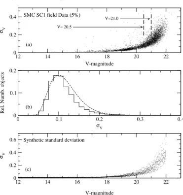
Appendix A: Photometric error simulations
As we selected the data using a criterion involving the photo-metric standard deviation of magnitude measurements, we have to generate an artificial standard deviation for the theoretical magnitude computed from evolutionary models. Moreover the general properties of the synthetic standard deviation distribu-tion must be similar to the OGLE 2 one.
We describe here the scheme used to generate the pseudo-synthetic photometric standard error distributions. The pre-fix “pseudo” means that we have extracted information about the standard error distribution from the OGLE 2 data them-selves (see Fig. A.1a). For that purpose, we divide the relevant range of magnitudes into bins; in each bin, we construct the histogram of standard deviation values (Fig. A.1b). This his-togram then is fitted with a function of the form:
P(σ)= a × (σ − σmin)4× e−b(σ−σmin)
where the constants a, b, σ, σminare derived from the OGLE 2
data. P(σ) represents the probability for having the standard deviation σ. The constants have been derived for each “mag-nitude bin”, for each OGLE fields in SMC and LMC. Then average values have been calculated over SMC and LMC.
In our population synthesis code, for a given magnitude value m, a standard deviation value σmis randomly determined
following the probability law derived from OGLE. After that, either the object is rejected (if the σm value is too large) or
12 14 16 18 20 22 V-magnitude 0 0.2 0.4 σV 0 0.1 0.2 0.3 0.4 σV 0 0.1 0.2
Rel. Numb. objects
12 14 16 18 20 22 V-magnitude 0 0.2 0.4 0.6 σV SMC SC1 field Data (5%) (a) (b) (c)
Synthetic standard deviation V= 20.5
V=21.0
Fig. A.1. a)Standard deviation σVversus V-magnitude for objects
be-longing to the SC1 field of the SMC. b) Histogram of the σV values
for magnitude V between 20.5 and 21.0, the fit (dashed curve) is per-formed with a function of a type given in the text. Differences between the fit and the histogram are clearly insignificant for our purpose. c)Synthetic σVdistribution generated with our algorithm.
the magnitude m is changed into mnoisy, following a gaussian
distribution having a standard deviation σm.
Let us comment about differences between Figs. A.1a and A.1c. Figure A.1a contains the “evolutionary information” – i.e. more objects at high magnitudes- whereas Fig. A.1c does not contain this information, objects have been uniformly dis-tributed with respect to the magnitude. These facts explain the difference between both figures.
References
Alexander, D., & Ferguson, J. 1994, ApJ, 437, 879
Alongi, M., Bertelli, G., Bressan, A., & Chiosi, C. 1991, A&A, 244, 95
Andersen, J. 1991, A&AR, 3, 91
Angulo, C., Arnould, M., Rayet, M., et al. 1999, Nucl. Phys. A, 656, 3 Bertelli, G., Bressan, A., Chiosi, C., Fagatto, F., & Nasi, E. 1994,
A&AS, 106, 275
B¨ohm-Vitense, E. 1958, Zs. f. Ap., 46, 135
Bressan, A. G., Chiosi, C., & Bertelli, G. 1981, A&A, 102, 25 Caughlan, G., & Fowler, W. 1988, Atomic Data Nuc. Data Tables, 40,
283
Caughlan, G., Fowler, W., Harris, M., & Zimmerman, B. 1985, Atomic Data Nuc. Data Tables, 32, 197
Charbonnel, C., Meynet, G., Maeder, A., & Schaerer, D. 1996, A&AS, 115, 339
Cioni, M.-R. L., Van der Marel, R. P., Loup, C., & Habing, H. J. 2000, A&A, 359, 601
de Jager, C., Nieuwenhuijzen, H., & van der Hucht, K. A. 1988, A&AS, 72, 259
Dutra, C. M., Bica, E., Clari´a, J. J., Piatti, A. E., & Ahumada, A. V. 2001, A&A, 371, 895
Eggleton, P., Faulkner, J., & Flannery, B. 1973, A&A, 23, 325 Flower, P. J. 1996, ApJ, 469, 355
Garcia, B., & Mermilliod, J. C. 2001, A&A, 368, 122
Gardiner, L. T., Hatzidimitriou, D., & Hawkins, M. R. S. 1991, Proc. Astron. Soc. Austr., 9, 80
Ghez, A. 1996, in Evolutionary processes in Binary Stars,
ed. R. A. M. J. Wijers, M. B. Davis, & C. A. Tout (Kluwer Academic Publishers), 1
Grevesse, N., & Noels, A. 1993, in Origin and Evolution of the Elements, ed. V.-F. E. Prantzos N., & C. M. (Cambridge University Press, Cambrigge), 14 (GN’93)
Grillmair Truc, T., & Truc, T. 1998, AJ, 115, 144
Groenewegen, M. A. T., & Salaris, M. 2001, A&A, 366, 752 Holtzman, Truc, T., & Truc, T. 1997, AJ, 113, 656
Iglesias, C. A., & Rogers, F. J. 1996, ApJ, 464, 943 (OPAL 96) Iwamoto, N., & Saio, H. 1999, ApJ, 521, 297
Izotov, Y., Thuan, T., & Lipovetsky, V. 1997, ApJS, 108, 1 Keller, S. C., Da Costa, G. S., & Bessell, M. S. 2001, AJ, 121, 905 Kov´acs, G. 2000, A&A, 363, L1
Kozhurina-Platais, V., Demarque, P., Platais, I., Orosz, J. A., & Barnes, S. 1997, AJ, 113, 1045
Kroupa, P., Tout, C., & Gilmore, G. 1993, MNRAS, 262, 545 Kudritzki, R., & Hummer, D. 1986, in IAU Symp. 116, Luminous
Stars and Associations in Galaxies, ed. P. L. C. de Loore, & A. J. Willis, 3
Landr´e, V., Prantzos, N., Aguer, P., et al. 1990, A&A, 240, 85 Laney, C. D., & Stobie, R. S. 1994, MNRAS, 266, 441 Lebreton, Y., Fernandes, J., & Lejeune, T. 2001, A&A, 374, 540 Lebreton, Y., Perrin, M.-N., Cayrel, R., Baglin, A., & Fernandes, J.
1999, A&A, 350, 587
Lejeune, T., Cuisinier, F., & Buser, R. 1997, A&AS, 125, 229 Lejeune, T., Cuisinier, F., & Buser, R. 1998, A&AS, 130, 65 Luck, R. E., Moffett, T. J., Barnes, T. G., & Gieren, W. P. 1998, AJ,
115, 605
Maeder, A., & Mermilliod, J. 1981, A&A, 93, 136 Maeder, A., & Meynet, G. 2001, A&A, 373, 555 Maeder, A., & Peytremann, E. 1970, A&A, 7, 120
Magee, N. H., Abdallah, J. Jr., Clark, R. E. H., et al. 1995, in Atomic Structure Calculations and New Los Alamos Astrophysical Opacities, ed. S. Adelman, & W. Wiese, vol. 78 (Astronomical Society of the Pacific Conf. Ser. (Astrophysical Applications of Powerful New Database)), 51
Massaguer, J. 1990, in Rotation and Mixing in Stellar Interiors, ed. M.-J. Goupil, & J.-P. Zahn (Springer, Berlin, Heidelberg, New York), 129
Mermilliod, J.-C., & Maeder, A. 1986, A&A, 158, 45 Morel, P. 1997, A&AS, 124, 597
Mould, J. R., Huchra, J. P., Freedman, W. L., et al. 2000, ApJ, 529, 786
Oestreicher, M. O., Gochermann, J., & Schmidt-Kaler, T. 1995, A&AS, 112, 495
Peimbert, M., Peimbert, A., & Ruiz, M. 2000, ApJ, 541, 688 Press, W., Teukolsky, S., Vetterling, W., & Flannery, B. 1992,
Numerical Recipes in Fortran 77 (Cambridge University Press) Ribas, I., Jordi, C., & Gim´enez, ´A. 2000, MNRAS, 318, L55 Rogers, F. J., & Iglesias, C. A. 1992, ApJS, 79, 507 Roxburgh, I. 1989, A&A, 211, 361
Salpeter, E. 1955, ApJ, 121, 161S
Schaller, G., Schaerer, D., Meynet, G., & Maeder, A. 1992, A&AS, 96, 269
Schlegel, D. J., Finkbeiner, D. P., & Davis, M. 1998, ApJ, 500, 525 Schr¨oder, K., Pols, O. R., & Eggleton, P. P. 1997, MNRAS, 285, 696 Stanek, K. Z., Zaritsky, D., & Harris, J. 1998, ApJ, 500, L141 Stothers, R. B., & Chin, C. 1991, ApJ, 381, L67
Talon, S., Zahn, J.-P., Maeder, A., & Meynet, G. 1997, A&A, 322, 209 Udalski, A., Soszynski, I., Szymanski, M., et al. 1999a, Acta Astron.,
49, 223
Udalski, A., Soszynski, I., Szymanski, M., et al. 1999b, Acta Astron., 49, 437
Udalski, A., Szyma´nski, M., Kubiak, M., et al. 1998, AcA, 48, 147 Udalski, A., Szyma´nski, M., Kubiak, M., et al. 2000, AcA, 50, 307 Vallenari, A., Chiosi, C., Bertelli, G., Aparicio, A., & Ortolani, S.
1996, A&A, 309, 367
Van der Marel, R. P., & Cioni, M. L. 2001, AJ, 122, 1807 Venn, K. 1999, ApJ, 518, 405
Wolff, S., & Simon, T. 1997, PASP, 109, 759 Zahn, J. 1991, A&A, 252, 179