Coupled surface-atmosphere reflectance (CSAR) model - Part 1 : Model description and inversion on synthetic data

HAL Id: hal-01989883

https://hal.uca.fr/hal-01989883

Submitted on 22 Mar 2021

HAL is a multi-disciplinary open access

archive for the deposit and dissemination of

sci-entific research documents, whether they are

pub-lished or not. The documents may come from

teaching and research institutions in France or

abroad, or from public or private research centers.

L’archive ouverte pluridisciplinaire HAL, est

destinée au dépôt et à la diffusion de documents

scientifiques de niveau recherche, publiés ou non,

émanant des établissements d’enseignement et de

recherche français ou étrangers, des laboratoires

publics ou privés.

Coupled surfaceatmosphere reflectance (CSAR) model

-Part 1 : Model description and inversion on synthetic

data

Hafizur Rahman, M.M. Verstraete, Bernard Pinty

To cite this version:

Hafizur Rahman, M.M. Verstraete, Bernard Pinty. Coupled surface-atmosphere reflectance (CSAR)

model - Part 1 : Model description and inversion on synthetic data. Journal of Geophysical Research,

American Geophysical Union, 1993. �hal-01989883�

JOURNAL OF GEOPHYSICAL RESEARCH, VOL. 98, NO. Dll, PAGES 20,779-20,789, NOVEMBER 20, 1993

Coupled Surface-Atmosphere Reflectance (CSAR) Model

1. Model Description and Inversion on Synthetic Data

HAFIZUR RAHMAN 1

Laboratoire d'Etudes et de Recherches en Tdl•ddtection Spatiale, Centre National de la Recherche Scientifique, Toulouse, France

MICHEL M. VERSTRAETE

Institute for Remote Sensing Applications, CEC Joint Research Centre, Ispra, Italy

BERNARD PINTY

Laboratoire de Mdt•orologie Physique, Centre National de la Recherche Scientifique, Universitd Blaise Pascal, Aubi•re, France Absorption and scattering processes in the atmosphere affect the transfer of solar radiation along its

double path between the Sun, the Earth's surface, and the satellite sensor. These effects must be taken

into account if reliable and accurate information on the surface must be retrieved from satellite remote

sensing data. One approach consists in characterizing the state of the atmosphere from independent observations and correcting the data with the help of radiation transfer models. This approach requires a detailed and accurate description of the composition of the atmosphere (e.g., aerosol and water vapor profiles in the case of advanced very high resolution radiometer data) at the time of the satellite overpass and requires significant computer resources. An alternative method is to attempt to simultaneously retrieve surface and atmospheric parameters by inverting a coupled surface- atmosphere model against remote sensing data. This study describes such a coupled model and the results of its inversion against synthetic data, using a nonlinear inversion technique. The results obtained are encouraging in that realistic directional reflectances at the top of the atmosphere can be produced, and the inversion of the model against these synthetic data is capable of estimating surface and atmospheric variables. The accuracy of the retrieval is studied as a function of the amount of noise added to the data. It is shown that some surface or atmospheric parameters are easier to retrieve than others with such a coupled model, and that although it appears to be difficult to accurately and reliably estimate the water vapor amount from channel 2, there is a definite possibility of retrieving the aerosol loading from simulated channel 1 data, if the type of aerosol can be assumed.

The scale, intensity, and persistence with which human activities have affected the environment and changed the composition of the atmosphere have raised questions about the sensitivity of the climate system to these perturbations and, in particular, about the likelihood of large-scale and long-term effects [Houghton et al., 1990; Jiiger and Fergu- son, 1991]. The widespread concern results from the fact that these changes may be unpredictable and largely unde- sirable. No consensus has been reached yet in the political arena on the need to take action, or even on the extent and severity of the measures that might be adopted, except that there is general agreement on the need for a much better understanding of the processes involved and for a reduction in the uncertainties associated with current predictions.

The most significant worldwide effort in this area is coordinated under aegis of the International Geosphere Biosphere Program (IGBP), also known as the Global Change Research Program [e.g., IGBP, 1988; National Academy of Sciences (NAS), 1988]. This research program

ion leave

from the Space

Research

and Remote

Sensing

Organi-

zation, Shere Bangla Nagar, Dhaka, Bangladesh. Copyright 1993 by the American Geophysical Union.

Paper number 93JD02071. 0148-0227/93/93 JD-02071 $05.00

13 •tltl•.,Ul•ttC[l d, lUUll[l d, 11UlIIUCl tJl pr or •tlC•tb, 1111•IUUIII• the modeling and monitoring of the global environment as well as the investigation of past changes to evaluate how the system has evolved under stress previously. This paper contributes to the overall objectives of these research pro- grams by proposing a new approach to the monitoring of terrestrial surfaces and of the atmosphere, using a coupled surface-atmosphere model to interpret existing satellite re- mote sensing data.

The development of remote sensing techniques has greatly improved our capability to monitor land surface processes. Specifically, large field of view satellites are able to observe the entire planet on a daily basis (advanced very high

resolution radiometer (AVHRR)) or even more frequently

(METEOSAT, GOES). Other more specialized satellites

offer a greater spatial or spectral resolution but less frequent

coverage (SPOT, LANDSAT) and can be used to support

detailed studies on smaller areas.

The principal scientific question that must be addressed in this context is the extraction of reliable, quantitative, accu- rate information on the surface or the atmosphere, or both, from radiation measurements made on board these satellites. For the purpose of this discussion, a remote sensing mea- surement in the optical spectral region can be considered a parametric function of n physical variables, where each of these variables is itself varying in space, in time, with the 20,779

20,780 RAHMAN ET AL.: COUPLED SURFACE-ATMOSPHERE REFLECTANCE MODEL, 1

wavelength of radiation, and with the geometric conditions

of illumination and viewing:

P----P(•I, •2, ''',

•n)

(1)

where •i - •/(x, t, A, O), i = 1, 2,...,

n, and wherex

represents

the various spatial coordinates,

t stands

for time,

A indicates the spectral dependency, and O refers to the

geometric conditions of illumination and observation

[e.g.,

Verstraete and Pinty, 1992]. Typical examples of these

variables •i would be the single-scattering

albedo or the

orientation of the scatterers constituting the observed me- dium. Since each individual remote sensing observation is a

complex function of multiple physical variables, it is not

possible,

in general, to retrieve the values of these variables

from a single measurement through simple analytical proce- dures. Measurements may be repeated, however, and a numerical inversion method may be used to estimate the

most probable

value of the physical variables,

i.e., the set of

variables that best explain the observed variability in the

data.

In principle, the variability in any one of the independent

variables (spatial, temporal, spectral

or angular)

can be used

to extract information on the medium under observation. Since each observable object (target) is characterized by a

particular absorption

spectrum,

spectral signatures

can be used to distinguish different targets. Similarly, the

spatial contrast (0p/0x) of the signal may be interpreted

in

terms of the geographical extent and distribution of these

objects, and the information contained in the temporal

domain (Op/Ot) can be used to describe

the dynamic evolu-

tion of the system. So far, the extraction of information on the basis of these variabilities has proceeded on the basis of

empirical relations (typically but not exclusively

with vege-

tation indices). Physically based models to describe the

angular variations of the signal (•p/OO) are much more

advanced, in part thanks to the level of understanding

that

has been acquired in the field of radiation transfer. For this reason, the angular variance of the signal has historically

been the principal source of information on the physical

processes

that must have produced

the observed

radiation.

Various authors have attempted to retrieve quantitative

information on the surface from an analysis of variations in the bidirectional reflectance of this surface [Goel and Deer-

ing, 1985;

Goel et al., 1984; Goel and Strebel, 1983;

Goel and

Thompson,

1984a, b, c; Pinty et al., 1989, 1990;

Dickinson

et al., 1990; Verstraete et al., 1990; Pinty and Verstraete, 1991a; Myneni and Ross, 1991]. The description and anal-

ysis of surface processes

is complicated,

however, by the

presence of the atmosphere, which may significanfiy

con-

taminate the measurements. Most works concerned with the

interpretation of directional effects assume that the data

does not significantly contribute to the observed reflectance

(laboratory or field measurements),

or that they have been

corrected to remove such effects.

The latter approach, however, is difi%ult to implement on an operational basis, because meaningful atmospheric cor- rections would require a rather detailed knowledge of the

state and composition

of the atmosphere

(in particular the

water vapor and aerosol content) at the time of the satellite overpass. While the precipitable water content of the atmo-

sphere can be obtained (albeit at a much coatset spatial

circulation models or from satellite observations in different

spectral bands, aerosol loading is essentially unknown.

Atmospheric

corrections

also imply the manipulation

of very

large data sets from two different sources

and raises signif-

icant computing issues.

Since these atmospheric effects are too large to ignore

[e.g., Kaufman, 1989] and rather difficult to remove on the

basis of ancillary data, a logical alternative is to attempt to retrieve simultaneously the relevant information on the

atmosphere

and the surface from the remote sensing

data

itself. This implies the design of a coupled surface- atmosphere model, and its inversion against these data to retrieve at once the properties of the atmospheric column

and those of the surface. A few authors have carried

investigations

in this area [e.g., Lee and Kaufman, 1986;

Liang and $trahler, 1993]. This paper also describes a

coupled

model (where the atmospheric

component

is simple

enough

to allow inversions

to take place) but focuses

on the

accuracy and reliability of the results obtained by inversion

of this coupled

model against

synthetic

data, as a function of

the level of noise in the data.

2. MODELING THE COUPLED SURFACE-ATMOSPHERE SYSTEM

Two specific

tools need to be developed

in order to exploit

the geometric

variability

in the remote sensing

data: a model

of the bidirectional reflectance of the surface and a model of

the contribution of the atmosphere to the measured reflec-

tance. These topics have been investigated

extensively

but

separately, and existing models will be adopted for the

current purpose.

2.1. Atmospheric Radiation Transfer Model

The radiation emitted by the Sun is absorbed and scattered

by various

atmospheric

constituents

on its way down to the

surface, where it is partially absorbed. The reflected portion is further affected (particularly by scattering) on its second

passage

through

the atmosphere,

before reaching

the satel-

lite sensor. These radiative processes in the atmosphere are relatively well known and have been extensively docu-

mented in the literature [e.g., Chandrasekhar, 1960; Leno-

ble, 1985]. They can be taken into account through the use of

a radiation transfer model and a description of the atmo-

spheric

profiles

of the relevant constituents.

In this study

we

used a parameterization

[Rahman and Dedieu, 1993] of the

5S model [Tanrg et al., 1983] and standard profiles corre- sponding to a continental atmosphere.

In practical applications,

the total radiation impinging

on

or emerging from a given medium is decomposed into a

direct component

(i.e., scattering

along the line defined

by

the source and the target, or the target and the sensor ) and a diffuse component (i.e., scattering from or in all direc-

tions). As discussed

by Tanrg et al. [1983], the consideration

of the various direct and diffuse contributions on the double

optical

path defined

by the relative location

of the Sun, the

surface and the satellite leads to the introduction of four different surface reflectances: the reflectance of direct and

diffuse

incoming

solar radiation, both directly into the satel-

lite sensor, and the reflectance of direct and diffuse incoming radiation, both indirectly reaching the instrument, after one

or more additional scattering events.

For the purpose

of simultaneously

retrieving atmospheric

RAHMAN ET AL.: COUPLED SURFACE-ATMOSPHERE REFLECTANCE MODEL, 1 20,781

the number of model parameters to a minimum (see section 3 below). However, it is well known that natural surfaces (and even the atmosphere itself) exhibit significant anisot- ropy (i.e., the reflectance of the coupled surface-atmosphere system is intimately dependent on the zenith and azimuth

angles of both the illumination and the viewing directions),

as a result of their varying optical and structural properties.

To satisfy these conflicting objectives (the accurate repre-

sentation of directional reflectances with a limited number of parameters), we have elected to represent the reflectance of the coupled system as follows:

Pt(01,

02,

t•)=

t•7{Pa(01,

02,

r(o)r(02)

{

+

1-fi(O1,

02,

&)S ps(Ol'

02'

-- Os(01,

02

, qb)]

fd(01)

+fd(02)

r(01

)

(2)

where t a is the gaseous

transmission

on the double

path and

Ps and Pa are the bidirectional reflectances of the surface and of the atmosphere, respectively. The effect resulting from diffuse directional illumination is represented through a parameterization of the surface reflectance as suggested by

Tanr• et al. [1983].

In this equation, 0• and 02 represent the illumination and viewing zenith angles; & is the relative azimuth; T(O•) and T(02) stand for the transmittance of the atmosphere on the

incoming and outgoing directions for the combined direct

and diffuse radiation, respectively; S is the spherical albedo of the atmosphere; and the multiplicative factor 1/(1 - fit(0•,

02, &)S) accounts for multiple reflections between the

surface and the atmosphere. fi is computed to represent the contribution of the bidirectional reflectance ps weighted by the angular-dependent diffuse irradiance and Tt• is the

atmospheric transmittance for direct radiation only. The

functions fd(Oi) represent the ratio of the diffuse to the total (direct and diffuse) solar radiation impinging on (i - 1) or emerging from (i = 2) the surface, at the specified zenith angle of illumination and observation, respectively:

Id(Oi)

fd(Oi) = i= 1, 2 (3)

ID(Oi) + Id(Oi)

where ID(Oi) and I•(Oi) represent the direct and diffuse solar

radiation fluxes.

Since the angular dependence of the diffuse irradiance is generally not known, we approximate fi, following Tanr• et

al. [1983], by

•(0•,

02, qb)•A + Bps(O 1, 02, qb)

(4)

where the coefficients A and B were estimated from radiative transfer calculations using realistic surface properties and

atmospheric conditions. In the specific case of the AVHRR sensor and for typical terrestrial surface conditions the authors suggest A = 0.331 and B = 0.032 for channel 1

(visible red band, 580 to 690 nm, for the NOAA 9 instrument) and A = 0.328 and B - 0.085 for channel 2 (near-infrared band, 720 to 970 nm, again for the NOAA 9 instrument). These coefficients apply for an average atmosphere, charac- terized by a typical continental aerosol optical thickness of 0.35. This expression yields a reasonable estimate of the contribution of the diffuse radiation to the total reflectance.

In (2) the direct and diffuse components of the radiation are well separated: the first term corresponds to the atmo-

spheric reflectance, the second term represents the bidirec- tional properties of the surface, and the third term approxi-

mates the contributions due to the diffuse part of the total signals.

Equation (2) clearly illustrates how the atmosphere mod-

ifies the anisotropy of the surface. In particular, the third

term (which is added to p•) of this equation smoothes the

bidirectional contribution of the surface in addition to the first term, by adding a component which couples the diffuse atmospheric and surface properties. Under atmospheric conditions where the scattering effects are limited (i.e., small

optical depth), the function fe tends to a small value and

since the atmospheric reflectance is also minimum, the surface angular anisotropy is directly transmitted to the top of the atmosphere without any significant perturbations. Equation (2) also implies that the reflectance taken immedi- ately above the surface is varying with the atmospheric conditions and depends on the scattering properties of the atmosphere with respect to the incoming radiation.

The atmospheric transmissions T(0•) and T(02) have been

estimated with a simple but accurate empirical model fitted to the 5S model of Tanrg et al. [1986], as explained by Rahman and Dedieu [1993]. This model takes into account the gaseous absorptions of ozone, water vapor, oxygen and carbon dioxide, as well as the scattering by molecules and aerosols. A standard continental aerosol profile, as de-

scribed in 5S, has been assumed. The model accepts as input

the zenith and azimuth angles of the illumination and viewing directions as well as the atmospheric contents of the radia- tively active constituents (water vapor, ozone, and aerosol). 2.2. Surface Bidirectional Reflectance Model

The bidirectional reflectance of the surface is simulated with the model of Verstraete et al. [1990], and Pinty et al. [1990]. This model calculates the directional reflectance emerging from an optically thick canopy or soil as a function

of the physical and structural properties of the surface and of

the angular positions of the Sun and of the observer. The optical and structural properties of the surface include the

single-scattering albedo and the phase function of the scat-

terers, their orientation, and a parameter describing the shape of the holes between the scattering elements. The

main advantages of this model are that (1) it is physically

based, i.e., the model parameters are precisely defined physical quantities; (2) the description of the hot spot (or opposition) effect derives naturally from the analytical com- putation of the transmission of radiation along the double path in the porous medium; (3) it uses only four physical parameters and can be inverted against actual or simulated data; and (4) it has been widely used and validated for a variety of soil and vegetation surfaces [Pinty et al., 1989, 1990; Jacquemoud et al., 1991].

Following Pinty et al. [1990], the bidirectional reflectance of a deep canopy is given by

20,782 RAHMAN ET AL.' COUPLED SURFACE-ATMOSPHERE REFLECTANCE MODEL, 1 0.12 0.11 0.1 0.0s 0.07 0.06 0.05 0.03 -6( do

Viewing Angle in the Principal Plane

Fig. la. Bidirectional reflectances computed in the principal plane for advanced very high resolution radiometer (AVHRR) channel 1' (asterisks) at the surface, (circles) top of the atmosphere with an aerosol optical depth at 550 nm of 0.1, (pluses) top of the atmosphere with an aerosol optical depth of 0.6. The scatterers are assumed to be uniformly distributed in orientation (Xl - 0) and the solar zenith angle is set at 20 ø. The other model parameters are •o = 0.2, 2rA = 1.0, {9 - 0, the ozone amount is assumed to be 0.3 cm atm, and the water vapor amount is 2.0 g cm -2.

proximates the contribution from multiple scattering [see Dickinson et al., 1990].

The functions K i represent the average cosine of the angles

between the normals to the scatterers and the direction of illumination (i = 1) or observation (i = 2). These values can be computed exactly if the statistical distribution of scatterer orientation is given [e.g., Verstraete, 1987], or can be estimated with simple empirical expressions, as suggested by Goudriaan [1977, 1988] or by Dickinson et al. [1990]. In the special simple case of uniformly distributed scatterers

(i.e., all scatterer orientations are equiprobable), Ki is con-

stant

and equal

to «. In the following

computations

we have

used the Henyey-Greenstein formula for the phase function P(#) [Pinty et al., 1990] and the parameterization of Dick-

inson et al. [1990] to estimate the •i functions.

The functions

Pv and Vp further

depend

on G, a geometric

factor that generally takes on large values, except when the direction of observation is close to the direction of illumina- tion, r, the radius of the Sun flecks on the inclined scatterers, a parameter related to the horizontal distance between the scatterers and A, the scatterer area density, expressed as the scatterer surface per unit bulk volume, a parameter related to the vertical spacing of the scatterers. Both r and A are relative to the field of view of the instrument and are therefore scale dependent.

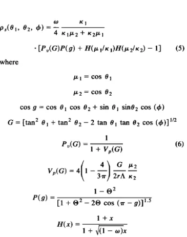
(.o K 1 Ps(01, 02, (•)--- 4 •1/•2 + •2/•1 ß [Pv(G)P(g) + H(/• 1/K 1)H(/•2/•2) - 1] (5) where COS 01 • 2 -- COS 02

COS g -- COS 01 COS 02 q- sin 01 sin02 COS (•)

G = [tan

2 01 q- tan2 02 -- 2 tan 01 tan 02 COS

(•)] 1/2

1 Pv(G) =

Vp(G)=4

1-

2rA

•2

[1 + 02- 20 cos (•r-g)]•'5

1 + d(1- w)x

In these equations, •o is the average single-scattering albedo

of the particles making up the surface; • and •2 are

describing the orientation distribution of the scatterers, for

the illumination and viewing angles, respectively; Pv(G) is

the function that accounts for the joint transmission of the incoming and outgoing radiation, and thereby also for the "hot spot" phenomenon; P(g) is the Henyey-Greenstein phase function of the scatterers; O is the phase function

parameter; and the expression H(l•l/Kl)H(l•2/g2) - 1 ap-

2.3. Sensitivity of the Anisotropy of the Coupled Model on Atmospheric Parameters

Absorption and scattering processes are strongly depen- dent on the wavelength of the radiation, both within the plant canopy and within the atmosphere (although differently so in each medium). As a result, the presence of the atmosphere

modifies the anisotropy patterns of the surface insofar as

they are observed by satellite instruments. In this section we

investigate this question specifically for channels 1 and 2 of

the AVHRR instrument. Channel 1 measurements are most sensitive to molecular scattering and to the nature and amount of aerosol. By contrast, channel 2 is mostly affected by water vapor absorption.

Figures l a and lb show the effect of changes in atmo- spheric aerosol optical thickness on the top of atmosphere directional reflectance, over a typical vegetation canopy

composed of isotropic scatterers ({9 - 0), as it would be

0.12 0.11 0.1 •o o.o8 •, 0.07 .,•

• 0.06

Viewing Angle in the Perpendicular Plane

RAHMAN ET AL.' COUPLED SURFACE-ATMOSPHERE REFLECTANCE MODEL, 1 20,783 0.22 0.2 0.18 • o.16 • 0.14

• 0.12

Viewing Angle in the Principal Plane

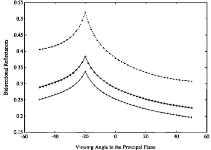
Fig. 2a. Same as Figure la except that © = -0.4.

sensed by AVHRR in channel 1, as a function of the view angle in the principal and perpendicular planes, respectively. The two different atmospheric conditions we considered are a relatively clear atmosphere with an aerosol optical depth at

0.55 •m of 0.1 and a more turbid atmosphere with aerosol

optical depth of 0.6; they are shown together with surface values (i.e., in the absence of atmospheric effects) for comparison. It can be seen that although the surface pattern clearly controls the shape of the function at the top of the atmosphere, the net effect of the atmosphere is not only to increase the reflectance (translation of the curves upward), but also to modify the angular distribution of the light (distorsion of the curves).

Figures 2a and 2b exhibit the same effect but this time for a scattering medium characterized by a more strongly back- scattering phase function (© = -0.4) such as would be observed for bare soils. In this case, a clear atmosphere does not significantly modify the bidirectional signal from the surface, but more turbid conditions appreciably reduce the directional variability of the signal, both in the principal and in the perpendicular planes.

These two sets of figures show that the net effect of the atmosphere can be to increase or decrease the angular variability of the reflected radiation field, depending on the

0.55 0.5 0.45 • 0.4 .• 0.35 .,• • 0.3 0.25 0.2 0.15 -6( -,•0 -•0 • 2•0 4'0 60

Viewing Angle in the Principal Plane

Fig. 3a. Bidirectional reflectances computed in the principal plane for AVHRR channel 2: (asterisks) at the surface, (circles) top of the atmosphere with a water vapor amount of 0.5 g cm-2, (pluses)

top of the atmosphere

with a water

vapor

amount

of 5.0 g cm-2; the

solar zenith angle is fixed at 20 ø . The other parameters are as

follows: •o = 0.8, Xt = 0, 2rA = 1.0, © = -0.2, the aerosol optical

depth at 550 nm is 0.3, and the ozone amount is 0.3 cm atm.

optical properties of the underlying surface and the turbidity

of the atmosphere.

The effect of atmospheric water vapor amount on the estimated directional reflectance for AVHRR channel 2 is shown in Figures 3a and 3b, again as a function of the viewing angle in the principal and perpendicular planes,

respectively. The water vapor contents are 0.5 and 5.0 g

cm -2, and the reflectances

at the surface

(i.e., in the absence

of the atmosphere) are shown for comparison. From this figure, it is clear that the atmospheric water vapor mostly

decreases the reflectance values for all viewing angles and does not introduce significant changes in the shape of the

anisotropy of the surface: Most of the directional variability

characterizing the surface is transmitted unaffected at the top of the atmosphere.

Obviously, these figures exhibit only a few of the many

possible combinations of surface and atmospheric properties that can be expected in nature, and it remains difficult to

draw general conclusions from these specific cases. How- ever, these simulations show that the atmosphere has the

0.22 0.2 0.18 0.16 0.14 0.12

0.1

Viewing Angle in the Perpendicular Plane

Fig. 2b. Same as Figure lb except that © = -0.4.

0.55 0.45 • 0.4 ,• 0.35 ..• • 0.3 0.25 0.2 0'15-60 -•0 -:J0 (• 2'0 4'0 60

Viewing Angle in the Perpendicular Plane

20,784 RAHMAN ET AL.: COUPLED SURFACE-ATMOSPHERE REFLECTANCE MODEL, 1

potential for modifying both the transmission and the angular distribution of light reflected by the surface:

(1) In the case of channel 1, where chlorophyll absorp-

tion leads to small reflectance values over vegetation cano- pies, atmospheric scattering modifies both the amplitude and

the angular distribution of the surface bidirectional reflec-

tance. Since the intrinsic reflectance of the atmosphere can reach values close to that of the surface, increasingly opti-

cally deep layers of atmospheric aerosol tend to smooth and mask the surface angular behavior.

(2) In the case of channel 2 the situation is much simpler

because the absorption process leads to a uniform reduction in the amplitude of the signal and large zenith angle condi-

tions must be considered before observing a significant change in the angular patterns of reflectance.

It must be pointed out here that it is this asymmetry in the

response of the two channels to atmospheric effects which is responsible for the anisotropic contamination of vegetation indices such as the normalized difference vegetation index by the atmosphere.

Although the effect of other absorbing gases such as

oxygen, carbon dioxide, and ozone have not been shown

here, their relative importance with respect to AVHRR

measurements lags behind that of the aerosol and water vapor content [Tanr• et al., 1992]. Since AVHRR measure- ments are strongly affected by these two atmospheric com- ponents (which also exhibit a large temporal and geograph- ical variability), it is reasonable to focus on them either when correcting the AVHRR data for the atmospheric masking

effects or when inverting a coupled surface-atmosphere model, as is the case in the present study. In the following

sections we discuss the invertibility of such a model and

examine the accuracy of the retrieved parameters which

result from the inversion.

3. DESCRIPTION OF THE INVERSION PROCEDURE

The fundamental issue in remote sensing is the retrieval of reliable accurate information about the target of interest

from an analysis of the measurements. Since each observa-

tion, in general, reflects the influence of multiple radiative

processes (e.g., emission and scattering), the extraction of

this information cannot be achieved analytically but relies

upon the inversion of mathematical models against multiple observations [e.g., Goel, 1988].

For the purpose of the discussion, let

z =f(x 1, X2, ''', Xn; Yl, Y2, ''' , Ym) (7) be an analytical representation (e.g., a reflectance model) of

the relation

between

the parameters

y j, (j = 1, ''' , m),

Each individual measurement of the observable quantity z

yields a value 5, which is presumably resulting from a

particular

set of values

of yj. Since

we usually

have m > 1

unknowns

and only one equation,

the values

of yj cannot

be

equations in M x m unknowns:

Zl =fl(Xll,

X12, ''',

Xln;

Yll, Y12, ''' , Ylm)

Z2--f2(x21, X22, ''', X2n; Y21, Y22, ''' , Y2m)

(8)

ZM--fM(XM1, XM2,' '', XMn;

YM•, YM2, ''',

YMm)

Additional assumptions are needed to solve such a system. Specifically, we will assume (1) that the target does not change significantly between measurements, i.e., that the

form of the equation

f and values

of the parameters

yj are

unchanged for all measurements, (2) that different observa-

tions, taken for various values of the independent variables xi, display significant variability, and (3) that more observa- tions are taken for various conditions x i than there are

parameters

yj to retrieve, i.e., M > m. Optionally,

one or

more of the parameters

yj can be specified

on the basis

of

other sources of information, in which case the number of

parameters

yj to be retrieved

by inversion

is decreased.

lem can be formulated as follows. Model inversion is a numerical procedure based on the iterative search for the global optimum of a figure of merit function. The sum of the squares of the differences between the observed values and those predicted by the model is often selected, in which case the function to minimize is

M

•2__

• Wi[•

i

i=1

- fi(xil, xi2, ''', Xin;

Yil, Yi2, ''', Yim)]

2 (9)

but other criteria could be used as well. The factors W i are

the weights given to the successive measurements. In this

study we have set Wi = 1 for all observations. In general, the larger the number of free model parameters the more difficult

it is to find a unique optimal solution. The models should

therefore be as simple as possible.

The mathematical tools to invert models are described in many standard texts [e.g., Press et al., 1992]. We routinely use the routine E04JAF of the Numerical Algorithms Group (NAG) library, which implements a quasi-Newton algorithm

to find the minimum

of the function/52

, subject

to upper

and

lower bounds on the independent variables. This algorithm uses function values only and searches for the optimum solution iteratively from an initial guess provided by the user. As always, when using packaged algorithms, it is up to the user to verify that all conditions required for the appli- cability of the program are fulfilled and that the results obtained are not sensitive to such things as the choice of initial guesses, the number of iterations, or the criteria used to stop the iteration process.

4. INVERSION OF THE COUPLED SURFACE-ATMOSPHERE

MODEL

In this section we demonstrate the feasibility of retrieving

both atmospheric and surface parameters from an inversion

of a coupled model against simulated satellite remote sensing data.

RAHMAN ET AL.' COUPLED SURFACE-ATMOSPHERE REFLECTANCE MODEL, 1 20,785

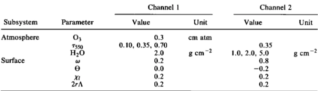
TABLE 1. Physical Parameter Values Used to Generate the Synthetic Data Sets

Subsystem

Channel 1 Channel 2

Parameter Value Unit Value Unit

Atmosphere Surface 0 3 0.3 cm atm r550 0.10, 0.35, 0.70 0.35 H20 2.0 g cm -2 1.0, 2.0, 5.0 to 0.2 0.8 0 0.0 -0.2 XI 0.2 0.2 2rA 0.2 0.2 g cm -2

4.1. Generation of Simulated Satellite Data

The coupled surface-atmosphere model described above was used to generate simulated AVHRR data at the level of the satellite, using the parameter values indicated in Table 1. Top of atmosphere reflectances were generated for solar

and view zenith angles from 0 ø to 50 ø, in steps of 10 ø, and for relative azimuth angles from 0 ø to 180 ø, in steps of 45 ø. The

basic data set therefore contain 180 reflectance values.

To investigate the inversion of a coupled model against

AVHRR-type data in the solar range, we generated a series

of data sets for different types of atmospheres. For AVHRR channel 1, both Rayleigh (molecular) and aerosol scattering

are relatively important. The former varies only slowly with

surface pressure, but the aerosol optical depth exhibits relatively large temporal and spatial variabilities. We have therefore generated three data sets corresponding to atmo-

spheres of different turbidities to simulate actual data in the

"visible" part of the spectrum: a relatively clear atmosphere with an aerosol optical depth r550 of 0.1, a moderate atmo- sphere with r550 = 0.35, and a more turbid atmosphere for which r550 - 0.7. In each of these three cases, the "true"

surface parameters were kept the same, and the other atmospheric parameters were kept at their nominal average

values, since they have little or no effect on atmospheric

transmission.

To generate data in the near-infrared band, we used a constant value of the aerosol optical thickness, since it is not a major variable in this spectral region. On the other hand, the presence of a water vapor absorption band affects the mea-

sured radiance at the top of the atmosphere and must be accounted for. In this case we have also generated three data

sets

for water vapor contents

of 1.0, 2.0, and 5.0 g cm -2,

eters were kept constant. All these data sets will be collectively

referred to as the "clean" data sets, to distinguish them from

the "noisy" data sets to be described below. 4.2. Method

Since it is difficult to accurately and reliably retrieve a large number of parameters from an inversion scheme, it is advisable to minimize this number in any one inversion. We

start by noting that if the aerosol loading affects both channels, the first one is the most sensitive to this atmo-

spheric constituent. At the same time, since the water vapor content modifies the measured radiances in channel 2 only, we take advantage of this decoupling to retrieve the aerosol loading from channel 1 first and impose this value while retrieving the water vapor amount from channel 2. For

analogous reasons we know a priori that the structural

properties of the surface (Xt and 2rA) should not be wave- length dependent, assuming that the canopy is vertically

homogeneous, and therefore should take on the same values in both channels. We also note that the generally low value of the single-scattering albedo w of leaves in the visible spectral region results in few multiple-scattering events, and thereby a more sharply defined anisotropy, than in the near

infrared. Since the anisotropy of the surface is largely

affected by the structure of the medium, we retrieve these parameters from inversion in the visible band and impose their values when performing the inversion in channel 2.

It follows that the inversion should be performed in

channel 1 first, to retrieve five parameters: the single scat- tering albedo w of the surface, the asymmetry factor of the

phase function ©, the scatterer orientation parameter Xt, the structural parameter 2rA, and the aerosol optical depth at 550 nm r550. The values of Xt, 2rA, and r550 are then imposed

during the inversion of the model against data in channel 2, which yields estimates for the single-scattering albedo w, the asymmetry factor of the phase function ©, and the water vapor content of the atmosphere. This approach minimizes the number of parameters to estimate at once and, inciden- tally, also reduces the computing requirements.

Actual measurements always include a certain amount of noise, and it is important to estimate how sensitive the results of an inversion are to the presence and amount of noise in the data. To this end, we have generated 500 noisy

data sets for each type of atmospheric condition and chan-

nel, by adding normally distributed random noise with zero mean and standard deviation of 0.1, 2.0, 4.0, 8.0, and 10.0% of the hemispherical reflectance value to the clean data sets described above. The same series of random numbers has been used for each value of the standard deviation. The coupled model was then inverted successively against each of these derived data sets, and these results have allowed the estimation of the mean value and standard deviation of each parameter, as a function of the amount of noise in the data.

A coefficient of variability rr i, also called "error sensitivity"

[Goel et al., 1984], has then been estimated as the ratio of these two quantities:

O' i = SD i/X i (10) where SD i is the standard deviation of the ith parameter and Xi is the average or true parameter value. This coefficient

provides an assessment of the variability of the retrieved canopy parameters when the reflectances are randomly modified, this statistic can be used to characterize the sensitivity of the parameter to noise in the data, and thereby

20,786 RAHMAN ET AL.' COUPLED SURFACE-ATMOSPHERE REFLECTANCE MODEL, I 0.9

0.7

....'"'

(b)

0.2

0 "

Fig. 4. Error sensitivity of the retrieved parameter values, for

AVHRR channel 1, as a function of the amount of noise in the data,

for an atmosphere with an aerosol optical depth of 0.1 at 550 nm. The four curves refer to (a) •o, (b) ,YI, (C) 2rA, and (d) r550.

the quality of the inversion procedure. The objective of this study on the effect of noise is to document the likely impact of instrumental and other sources of imprecision on the results of the inversion. A different representation of noise would probably affect the results differently. In the next two sections we apply this approach to data sets simulating AVHRR channels 1 and 2.

4.3. Inversion Against Synthetic Data for Channel 1 of Advanced Very High Resolution Radiometer (AVHRR)

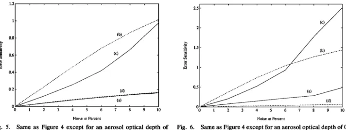
The error sensitivity tr i, defined above, is shown in

Figures 4, 5, and 6 for three different atmospheres, differing only by the aerosol optical depth, as a function of the amount of noise in the data.

The estimation of the single-scattering albedo to turns out to be quite robust with respect to the level of noise in the data. The corresponding error sensitivity increases slightly with increasing noise level and depends somewhat on the type of atmosphere. With a noise level of 10% the error sensitivity is 0.13 for a clear atmosphere, whereas for a moderate or a turbid atmosphere the values are 0.16 and 0.49, respectively. In generating channel 1 data, we have

assumed isotropic scatterers (i.e., an asymmetry factor O = 0), so we cannot calculate the error sensitivity for this parameter. However, independently of atmospheric turbid- ity the standard deviation of this parameter is about 0.005, which is a very small value. When the noise level is increased to 10%, the standard deviation reaches 0.03. The

leaf orientation parameter Xl is one of the two structural

parameters of the surface. The corresponding error sensitiv- ity shows a similar behavior as that of the single-scattering albedo: it increases with increasing noise level for the three types of atmospheres, but much more rapidly than for the former parameter, and increases with the aerosol load. When the noise level in the synthetic data reaches 10%, the error sensitivities are 0.85, 1.01, and 1.4 for a clear, moder- ate, and turbid atmosphere, respectively.

A relatively unstable behavior is observed for the other structural parameter 2rA, in which the error sensitivity increases relatively rapidly with the increasing noise level in the data, for the three types of atmospheres. The corre- sponding error sensitivities are 0.6, 0.98, and 2.5 for a clear, average, and turbid atmosphere, respectively, and for a noise level of 10% in each case. The error sensitivity for the aerosol optical depth seems relatively stable with respect to the noise introduced in the data, with values of 0.46, 0.16, and 0.06 corresponding to a clear, moderate, and turbid atmosphere, again for a noise of 10% in the data. In fact, this result shows that this parameter is almost unaffected by the noise level up to 10% and can be easily retrieved by the inversion technique.

In summary, the optical parameters of the surface and the aerosol loading in the atmosphere appear to be retrievable even from noisy data, while the morphological parameters of the canopy appear to be the more difficult ones to estimate in the presence of noise. Two remarks must be made in this respect, although they are not pursued further in this paper: (1) if the angular sampling scheme to observe the bidirec- tional reflectance field is flexible, it may be quite useful to increase the density of observations at small phase angles, to improve the accuracy and reliability of the retrieval of the structural parameters, and (2) if this sampling scheme is not flexible (as is usually the case for satellite instruments) or if few or no observations are made at small phase angles, the accuracy of the retrieval of the hot spot parameter may be very low if the data are very noisy.

• 0.6

0.4

0.2

...•

'•f•

(a)

Fig. 5. Same as Figure 4 except for an aerosol optical depth of

0.35 at 550 nm. 2.5 '•- 1.5 0.5 _ 1 2 3 4 5 6 7 8 9 10 Noise in Percent

Fig. 6. Same as Figure 4 except for an aerosol optical depth of 0.7

RAHMAN ET AL.' COUPLED SURFACE-ATMOSPHERE REFLECTANCE MODEL, 1 20,787

4.4 Inversion Against Synthetic Data for Channel 2 of A VHRR

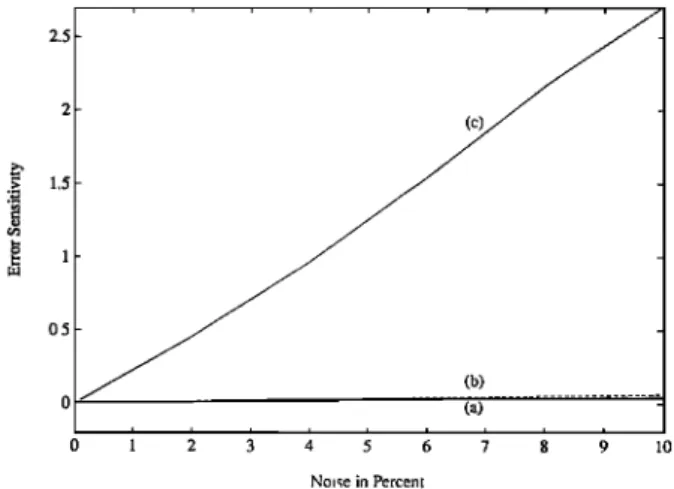
Just as was done above for channel 1, Figures 7, 8, and 9 show the results of repeated inversions of the coupled surface-atmosphere model against 500 instances of synthetic noisy data sets. The three different atmospheric conditions considered here correspond to water vapor contents of 1.0,

2.0, and 5.0 g cm -2. The panels

exhibit

the error sensitivities

of the different parameters, also as a function of the amount of noise.

For all practical purposes the retrieved values of single- scattering albedo to are not significantly affected by the level of noise introduced in the data, irrespective of the amount of atmospheric water vapor. The error sensitivity for this parameter is also very small for the three values of atmo- spheric water vapor content, although a slight increase is observed with the increase of noise in the data. With a noise level of 10% the corresponding values of the error sensitiv- ities are 0.043, 0.046, and 0.046 for an atmosphere having a

water content

1.0, 2.0, and 5.0 g cm -2 respectively.

The retrieval accuracy of the asymmetry factor © is also very encouraging, since it is almost independent of the noise

level in the data (up to 10%, for three different water vapor

contents in the atmosphere). In fact, for a noise level ranging from 0.1 to 10%, the performance is almost the same. The error sensitivity is also rather small for this parameter in all three cases of atmospheric water vapor content: of the order

of 0.06 for a noise of 10%, which indicates that this param-

eter can reliably be retrieved by inversion, even when the data are noisy.

On the other hand, the retrieved values of water vapor content show a high dependency on the level of noise in the data. The difficulty to retrieve accurate and reliable esti- mates of this parameter in the presence of noise in the data is confirmed by the error sensitivity statistics, which in- creases very rapidly with the level of noise. Furthermore, this effect is more pronounced for smaller water vapor

content

(1.0 g cm -2) than for higher

amounts.

The corre-

sponding values of error sensitivities are 2.7, 1.7, and 0.75

for a noise level of 10% and for atmospheres having water

vapor content

1.0, 2.0, and 5.0 g cm -2, respectively.

When

2.5 0.5 , , (c) (b) ... 0 1 2 3 4 5 6 7 8 9 10 Noise in Percent

Fig. 7. Error sensitivity of the retrieved parameter values, for AVHRR channel 2, as a function of the amount of noise in the data, for an atmosphere with a water vapor amount of 1.0 g cm -2. The different curves correspond to different parameters, keyed as fol- lows: (a) to, (b) ©, and (c) water vapor amount.

0.5

... 57! ...

(a)

0

•

2

3

4

5

6

7

i

;

10

Noise in Percent

Fig. 8. Same as Figure 7 except for a water vapor content of 2.0 g

-2 cm

the noise level drops to 0.1%, the corresponding values of

error sensitivity are only 0.02, 0.017, and 0.01, respectively,

for the same atmospheres. Clearly, the atmospheric water vapor content is very difficult to retrieve from noisy data with this technique, unless very precise reflectance measure- ments are made by space instruments.

5. CONCLUSIONS

Various remarks may be made on the series of experi- ments described in this paper: First, it is possible to design and implement coupled surface-atmosphere models to rep- resent the anisotropy of the total system and yet simple enough to be inverted jointly against simulated satellite data. A parametric model such as this one must be seen as an approximation to the full treatment of the radiation transfer in a medium with two superposed layers. In the specific case envisaged here, the atmospheric medium is well understood and the only unknown optical property is the optical depth of the variable optically active elements. Clearly, in the ap- proach described here and by opposition to the approaches

developed earlier, more importance has been given to the

proper representation of the surface than to that of the atmosphere.

Second, an analysis of the inversion results has shown that

0.8 0.6 0.4 0.2 -0.2

(c)

•

(b)

...

Fig. 9. Same as Figure 7 except for a water vapor content of 5.0 g

-2 cm

20,788 RAHMAN ET AL.: COUPLED SURFACE-ATMOSPHERE REFLECTANCE MODEL, 1

the variance associated with the noise in the data does not affect the retrieval of all physical parameters equally. Spe- cifically, some of the parameters can be retrieved with good accuracy, even from noisy data, while others are much more difficult to estimate at an acceptable level of accuracy. Since the accuracy of the results depends on the angular sampling of the bidirectional reflectance of the joint surface- atmosphere system as well as the level of noise in the measurements, sampling strategies and the quality of the instruments will have to be designed as a function of the

particular scientific objectives being pursued. For instance,

AVHRR data may prove to be adequate for retrieving the single-scattering albedo of the surface, in both channels, but not the water vapor amount, unless numerous high-quality data are collected for the particular location and time of interest.

Third, and perhaps most importantly, it has been shown that atmospheric corrections are not, in principle, the only way to account for the masking effect of the atmosphere. Since these corrections always necessitate rather severe

hypotheses, such as an average typical atmospheric profile,

or rely on large data sets to describe the state of the atmosphere from independent observations, they always represent a rather cumbersome operation. The develop- ments described in this paper show that it may be possible to retrieve atmospheric parameters simultaneously with sur- face characteristics, provided that sufficient sampling of the bidirectional reflectance distribution and accurate reliable data can be obtained. The multiangle imaging spectroradi- ometer instrument on board the upcoming AM platform of

NASA may significantly improve our data acquisition capa-

bility in this respect [Diner et al., 1979].

Specifically, it is suggested that (1) if the surface bidirec- tional reflectance exhibits a strong hot spot and this angular region is adequately sampled, then the optical and the structural properties of the surface may be retrieved with good accuracy; (2) if the surface does not exhibit such a hot spot, or if it does but the angular sampling is not sufficient in that region, then the optical properties of the surface and possibly the average orientation of the scatterers may be reliably retrieved, but the structure of the canopy cannot be accurately assessed. Furthermore, (3) the estimation of the aerosol loading of the atmosphere appears to be feasible in principle from channel 1 of AVHRR, if the type of aerosol can be assumed (e.g., continental) and if the aerosol loading

is large enough, even in the presence of appreciable noise in

the data, while (4) the accurate retrieval of the atmospheric

water vapor amount from channel 2 data appears difficult,

unless the data are of very high quality.

Clearly, the design of the AVHRR instrument and in particular the position of its channels were not selected to retrieve surface and atmospheric properties in the way described above. Rather, the existence of long series of AVHRR observations and the properties of its wide spectral bands have generated a strong interest in the climatological and ecological communities toward the use of these data to document climatic and environmental changes. It is unfor- tunate that the atmospheric water vapor cannot be easily and simply retrieved from AVHRR channel 2 data, but this parameter is generally rather well known, as it is measured

independently by the upper air meteorological stations, or

from other remote sensing instruments (such as TOVS, also located on the NOAA satellite).

If new and better atmospheric sounders will be designed and launched in the near future and will provide an adequate description of the distribution of water vapor in the atmo- sphere, the aerosol loading of the atmosphere has always

been and will continue to be a major unknown and a

significant perturbing factor for the analysis of data in channel 1 of AVHRR. The prospect of being able to retrieve a useful estimate of this loading from the inversion of a coupled model against these data is therefore most exciting. Of course, this opportunity may materialize only to the extent that accurate data may become available. The new generation of sensors should result in major advances, as noted above.

This paper describes only preliminary results from a simulation study. This work must now be carried over to actual AVHRR data to demonstrate the validity of the approach advocated here. This will require a different model to describe the anisotropy of the surface, because actual

ecosystems do not generally satisfy the homogeneity criteria

assumed by the surface model used here. These issues will be addressed in a companion paper.

Acknowledgments. The authors are grateful to Yoram Kaufman and the anonymous reviewers of this paper for their thorough and constructive comments. This work would not have been possible without the financial support of the French Programme National de T616d6tection Spatiale (PNTS). M. Verstraete also acknowledges the continuing support of the global change activity in the specific programme and the Exploratory Research program of the CEC Joint

Research Centre.

REFERENCES

Chandrasekhar, S., Radiative Transfer, 393 pp., Dover, Mineola, N.Y., 1960.

Dickinson, R. E., B. Pinty, and M. M. Verstraete, Relating surface albedos in GCM to remotely sensed data, Agric. For. Meteorol.,

52, 109-131, 1990.

Diner, D. J., et al., MISR: A multiangle imaging spectroradiometer for geophysical and climatological research from EOS, IEEE

Trans. Geosci. Remote $ens., GE-27, 200-214, 1989.

Goel, N. S., Models of vegetation canopy reflectance and their use in estimation of biophysical parameters from reflectance data,

Remote $ens. Rev., 4, 1-212, 1988.

Goel, N. S., and D. W. Deering, Evaluation of a canopy reflectance model for LAI estimation through its inversion, IEEE Trans.

Geosci. Remote $ens., GE 23,674-684, 1985.

Goel, N. S., and D. E. Strebel, Inversion of vegetation canopy reflectance models for estimating agronomic variables, I, Problem definition and initial results using Suit's model, Remote $ens.

Environ., 13,487-507, 1983.

Goel, N. S., and R. L. Thompson, Inversion of vegetation canopy reflectance models for estimating agronomic variables, III, Esti- mation using only canopy reflectance data as illustrated by the Suits' model, Remote Sens. Environ., 15,223-236, 1984a. Goel, N. S., and R. L. Thompson, Inversion of vegetation canopy

reflectance models for estimating agronomic variables, IV, Total

inversion of the SAIL model, Remote Sens. Environ., 15, 237- 253, 1984b.

Goel, N. S., and R. L. Thompson, Inversion of vegetation canopy reflectance models for estimating agronomic variables, V, Esti- mation of LAI and average leaf angle using measured canopy

reflectances, Remote $ens. Environ., 16, 69-85, 1984c.

Goel, N. S., D. E. Strebel, and R. L. Thompson, Inversion of vegetation canopy reflectance models for estimating agronomic variables, II, Use of angle transforms and error analysis as illustrated by the Suits' model, Remote $ens. Environ., 14,

77-111, 1984.

Goudriaan, J., Crop Micrometeorology: A Simulation Study, Wa- geningen Center for Agricultural Publishing and Documentation, Wageningen, Netherlands, 1977.