Role of the Arctic snow cover in high-latitude hydrological cycle asrevealed by climate model simulations

(1)

HAL Id: tel-02459108

https://tel.archives-ouvertes.fr/tel-02459108

Submitted on 29 Jan 2020

HAL is a multi-disciplinary open access

archive for the deposit and dissemination of sci-entific research documents, whether they are pub-lished or not. The documents may come from teaching and research institutions in France or abroad, or from public or private research centers.

L’archive ouverte pluridisciplinaire HAL, est destinée au dépôt et à la diffusion de documents scientifiques de niveau recherche, publiés ou non, émanant des établissements d’enseignement et de recherche français ou étrangers, des laboratoires publics ou privés.

Role of the Arctic snow cover in high-latitude

hydrological cycle asrevealed by climate model

simulations

Maria Santolaria Otin

To cite this version:

Maria Santolaria Otin. Role of the Arctic snow cover in high-latitude hydrological cycle asrevealed by climate model simulations. Climatology. Université Grenoble Alpes, 2019. English. �NNT : 2019GREAU027�. �tel-02459108�

(2)

DOCTEUR DE L

_{A COMMUNAUTÉ UNIVERSITÉ}

GRENOBLE ALPES

Spécialité : Sciences de la Terre et de l'Univers et de l'Environnement (CESTUE)

Arrêté ministériel : 25 mai 2016

Présentée par

María SANTOLARIA OTIN

Thèse dirigée par Olga ZOLINA, Enseignant-chercheur, Communauté Université Grenoble Alpes

préparée au sein du Laboratoire Institut des Géosciences de

l'Environnement

dans l'École Doctorale Terre, Univers, Environnement

Le rôle de la couverture de neige de

l'Arctique dans le cycle hydrologique de

hautes latitudes révélé par les simulations

des modèles climatiques

Role of the Arctic snow cover in high-latitude

hydrological cycle as revealed by climate

model simulations

Thèse soutenue publiquement le 4 novembre 2019, devant le jury composé de :

Madame OLGA ZOLINA

MAITRE DE CONFERENCES, UNIVERSITE GRENOBLE ALPES, Directeur de thèse

Monsieur PAVEL GROISMAN

DOCTEUR EN SCIENCES, SCIENCES & SCE. D'HYDROLOGIE-ASHEVILLE, Rapporteur

Monsieur NOEL KEENLYSIDE

PROFESSEUR, UNIVERSITE BERGEN - NORVEGE, Rapporteur Monsieur GERHARD KRINNER

DIRECTEUR DE RECHERCHE, CNRS DELEGATION ALPES, Président Monsieur MARTIN WEGMANN

DOCTEUR EN SCIENCES, INSTITUT ALFRED WEGENER ALLEMAGNE, Examinateur

Monsieur SERGEY GULEV

(3)

(4)

(5)

‘La filosof´ıa está escrita en ese libro enorme que tenemos continuamente abierto delante de nuestros ojos (hablo del universo), pero que no puede entenderse si no aprendemos primero a comprender la lengua y a conocer los caracteres con que se ha escrito. Está escrito en lengua matemática, y los caracteres son triángulos, c´ırculos y otras figuras geométricas sin los cuales es

humanamente imposible entender una palabra ; sin ellos se deambula en vano por un laberinto oscuro.”

“Il saggiatore”, Galileo Galilei (1623)

(6)

(7)

Remerciements

During these three years, ma vie s’est d´eroul´ee toujours dans trois langues. As´ı que en mis agradecimientos vais a tener que entrar en mi cabeza . . .

First, I would like to thank my supervisor, Olga Zolina, for the trust and confidence that she has put in me during these three years. I have felt free and guided to fully explore the Arctic. I am very thankful to the rapporteurs of this PhD, Noel Keenlyside and Pavel Groisman, for accepting the review of the manuscript. In particular, I would like to thank Noel Keenlyside for inviting me to Bergen, and to give me such a warm welcome in his team. I acknowledge the serenity and the wise advice of Pavel Groisman, they have been always very pertinent and useful for my research. I am very thankful to rest of jury : Gerhard Krinner, for sharing his endless wisdom of the CMIP world ; Sergey Gulev, for looking after my PhD since the very beginning and Martin Wegmann, for all his support and motivation over these three years. I would like to thank also the members of the ARCTIC-ERA Project, it has been always a pleasure to meet them all over the world. In particular, I thank Dmitry Streletskiy to make me discover the real permafrost of the Arctic Tundra.

Il me tient à cœur de remercier Martin Ménégoz, qui m’a aidée à faire les premiers pas au BSC et qui m’a introduite à ce merveilleux monde de la cryosphere.

Je dédie un grand remerciement à Ambroise Dufour, pour les trois années partagées entre lignes de code, transmission d’expérience et savoir et surtout, pour sa sérénité et sa précieuse et incalculable aide sur la fin.

Ç a a été un grand plaisir d’avoir été entouré de glaciologues, climatologues, nivologues et même des sismologues pendant ces trois ans. Dans ce labo, on sent que les différents chemins de recherche se croisent ainsi que les différentes passions. Je voudrais remercier tous les gens du labo qui m’ont encouragée surtout dans la dernière ligne droite avec des petits mots echangés dans les couloirs. Les sourires du publique de la Salle Llibourty le jour de ma soutenance, toutes les félicitations et les discussions d’après donnent vraiment envie de partager ton travail, elles te font sentir que, en fait, tu appartiens aussi à cette communauté scientifique.

“Les jours passent vite quand on s’amuse” et c’est ce qui s’est passé : les midis à EVE, les soirées au Labo (“le bon”), les weekends en montagne, dans les Calanques ou n’importe où mais haut, donnent des très bons souvenirs, et tout ¸ca c’est grâce à la bonne ambiance entre tous les

(8)

doctorants (et pas que) du labo. C’était un grand plaisir de partager ces trois ans avec mes collègues de promo : Jai, Marion, Lucas et Kévin. On l’a super bien réussi, bravo à nous tous ! Je pense que chacun a apporté son truc à cette mini équipe. Aussi, je tiens à remercier les “anciens” doctorants qui nous balisent le chemin (Etienne, Olivier, Fanny, Ilan, Cédric, Julien Beaumet, Joseph . . .) ainsi qu’aux “nouveaux” doctorants qui apportent de la fraˆıcheur dans le laboratoire (Ugo, Jordi, Sarah. . .). Quelques mots spéciaux pour mes très chères co-bureaux Jinhwa Shin et Albane Barbero : j’ai eu une chance énorme d’être tombée dans ce bureau (même si ¸ca caille en hiver) et d’avoir pu partager avec vous nos intimes inquiètudes et joies (“Wait wait, close the door !”). Gabi, mi querida menina, no sé que hubiese hecho sin ti. También va para ti Marta, por esos vinitos a -2 ◦C en la terraza de Place Saint Eynard, arreglando el mundo as´ı como si nada.

Esta tesis también va dedicada a todas mis amigas de Huesca, que han escuchado mis chapadas sobre el cambio climático y el Ártico con los ojos y o´ıdos abiertos durante todos estos años. Y sobre todo, durante este largo verano, por hacerme olvidar el manuscrito durante un ratito en compan´ıa de unos buenos kikos y una caña fresquita en el Candolias. Todo este esfuerzo no hubiese sido posible sin mi familia. Mil gracias a mi T´ıa Chus, a Jota y a Santi por venir a verme a esta ciudad lejana entre montañas. Muchas gracias a Laura por la ayuda log´ıstica y culinaria. Es fácil volar sin alas cuando tienes un buen paraca´ıdas, y eso es lo que son mi madre, mi padre y mi hermano. Quizás sin saberlo, cada uno ha aportado su grano de arena a este trabajo y a su autora : la pasión y la alegr´ıa de mi madre, la razón y calma de mi padre y la experiencia y creatividad cient´ıfica de mi hermano. Con todo esto no se puede fallar. Y por último pero no menos importante, merci Julien Brondex, tu m’a toujours apporté la lumière dans cette longue course.

(9)

R´

esum´

e

La neige est une composante essentielle du syst`eme climatique arctique. Au nord de

l’Eurasie et de l’Amérique du Nord, la couverture neigeuse est présente de 7 à 10 mois par an et son extension saisonnière maximale représente plus de 40% de la surface terrestre de l’hémisphère nord. La neige affecte une variété de processus climatiques et de rétroactions aux hautes latitudes. Sa forte réflectivité et sa faible conductivité thermique ont un effet de refroidissement et modulent la rétroaction neige-albédo. Sa contribution au bilan radiatif de la Terre est comparable à celle de la banquise. De plus, en empêchant d’importantes pertes d’énergie du sol sous-jacent, la neige limite la progression de la glace et le développement du pergélisol saisonnier. Réserve d’eau naturelle, la neige joue un rôle essentiel dans le cycle hydrologique aux hautes latitudes, notamment en ce qui concerne l’évaporation et le ruissel-lement. La neige est l’une des composantes du système climatique présentant la plus forte variabilité. Le réchauffement de l’Arctique étant deux fois plus rapide que celui du reste du globe, la variabilité présente et future des caractéristiques de la neige est cruciale pour une meilleure compréhension des processus et des changements climatiques. Cependant, notre ca-pacité à observer l’Arctique terrestre étant limitée, les modèles climatiques jouent un rôle clé dans notre aptitude à comprendre les processus liés à la neige. À cet égard, la représentation des rétroactions associées à la neige dans les modèles climatiques, en particulier pendant les saisons intermédiaires (lorsque la couverture neigeuse de l’Arctique présente la plus forte variabilité), est primordiale.

Notre étude porte principalement sur la représentation de la neige terrestre arctique dans les modèles de circulation générale issus du projet CMIP5 (Coupled Model Intercomparison Project) au cours du printemps (mars-avril) et de l’automne (octobre-novembre) de 1979 à 2005. Les caractéristiques de la neige des modèles de circulation générale ont été validées par rapport aux mesures de neige in situ, ainsi qu’à des produits satellitaires et à des réanalyses. Nous avons constaté que les caractéristiques de la neige dans les modèles ont un biais plus marqué au printemps qu’en automne. Le cycle annuel de la couverture neigeuse est bien reproduit par les modèles. Cependant, les cycles annuels d’équivalent en eau de la neige et de sa profondeur sont largement surestimés par les modèles, notamment en Amérique du Nord. Il y a un meilleur accord entre les modèles et les observations dans la position de la marge de neige au printemps plutôt qu’en automne. Les amplitudes de variabilité interannuelle pour toutes les variables de la neige sont nettement sous-estimées par la plupart des modèles CMIP5. Pour les deux saisons, les tendances des variables de la neige dans les modèles sont principalement négatives, mais plus faibles et moins significatives que celles observées. Les distributions spatiales des tendances de la couverture neigeuse sont relativement bien reproduites par les modèles, toutefois, la distribution spatiale des tendances en équivalent-eau et en profondeur de la neige présente de fortes hétérogénéités régionales.

Enfin, nous concluons que les modèles CMIP5 fournissent des informations précieuses sur les caractéristiques de la neige en Arctique terrestre, mais qu’ils présentent encore des limites. Il y a un manque d’accord entre l’ensemble des modèles sur la distribution spatiale de la neige par rapport aux observations et aux réanalyses. Ces écarts sont particulièrement marqués dans les régions où la variabilité de la neige est la plus forte. Notre objectif dans cette étude était d’identifier les circonstances dans lesquelles ces modèles reproduisent ou non les caractéristiques observées de la neige en Arctique. Nous attirons l’attention de la communauté scientifique sur la nécessité de prendre compte nos résultats pour les futures études climatiques.

(10)

Mots clés : Caractéristiques de la neige, climat arctique, modèles CMIP5, réanalyses, stations de neige.

(11)

Abstract

Snow is a critical component of the Arctic climate system. Over Northern Eurasia and North America the duration of snow cover is 7 to 10 months per year and a maximum snow extension is over 40% of the Northern Hemisphere land each year. Snow affects a variety of high latitude climate processes and feedbacks. High reflectivity of snow and low thermal conductivity have a cooling effect and modulates the snow-albedo feedback. A contribution from terrestrial snow to the Earth’s radiation budget at the top of the atmosphere is close to that from the sea ice. Snow also prevents large energy losses from the underlying soil and notably the ice growth and the development of seasonal permafrost. Being a natural water storage, snow plays a critical role in high latitude hydrological cycle, including evaporation and run-off. Snow is also one of the most variable components of climate system. With the Arctic warming twice as fast as the globe, the present and future variability of snow characteristics are crucially important for better understanding of the processes and changes undergoing with climate. However, our capacity to observe the terrestrial Arctic is limited compared to the mid-latitudes and climate models play very important role in our ability to understand the snow-related processes especially in the context of a warming cryosphere. In this respect representation of snow-associated feedbacks in climate models, especially during the shoulder seasons (when Arctic snow cover exhibits the strongest variability) is of a special interest.

The focus of this study is on the representation of the Arctic terrestrial snow in global circulation models from Coupled Model Intercomparison Project (CMIP5) ensemble during the melting (March-April) and the onset (October-November) season for the period from 1979 to 2005. Snow characteristics from the general circulation models have been validated against in situ snow measurements, different satellite-based products and reanalyses.

We found that snow characteristics in models have stronger bias in spring than in autumn. The annual cycle of snow cover is well captured by models in comparison with observations, however, the annual cycles of snow water equivalent and snow depth are largely overestima-ted by models, especially in North America. There is better agreement between models and observations in the snow margin position in spring rather than in autumn. Magnitudes of interannual variability for all snow characteristics are significantly underestimated in most CMIP5 models compared to observations. For both seasons, trends of snow characteristics in models are primarily negative but weaker and less significant than those from observa-tions. The patterns of snow cover trends are relatively well reproduced in models, however, the spatial distribution of trends for snow water equivalent and snow depth display strong regional heterogeneities.

Finally, we have concluded CMIP5 general circulation models provides valuable infor-mation about the snow characteristics in the terrestrial Arctic, however, they have still limitations. There is a lack of agreement among the ensemble of models in the spatial dis-tribution of snow compared to the observations and reanalysis. And these discrepancies are accentuated in regions where variability of snow is higher in areas with complex terrain such as Canada and Alaska and during the melting and the onset season. Our goal in this study was to identify where and when these models are or are not reproducing the real snow cha-racteristics in the Arctic, thus we hope that our results should be considered when using these snow-related variables from CMIP5 historical output in future climate studies.

(12)

Keywords : Snow characteristics, Arctic climate, CMIP5 models, reanalyses, rnow sta-tions.

(13)

Notations

The acronyms and the main abbreviations used in this PhD are shown below.

Acronyme Signification

ACIA Arctic Climate Impact Assessment

AMIP Atmosphere Model Intercomparison Project AMO Atlantic Multidecadal Oscillation

AO Arctic Oscillation

AOGCM Atmosphere-Ocean General Circulation Model AVHRR Advanced Very High Resolution Radiometer CAVM Circumpolar Arctic Vegetation Map

CDO Climate Data Operator

CDR Climate Data Record

CIRES Cooperative Institute for Research in Environmental Sciences

CLM Community Land Model

CMIP5 Coupled Model Intercomparison Project 5 CMOR Climate Model Output Rewriter

DAS Data Assimilation System

ECMWF European Centre for Medium-Range Weather Forecasts

EDLB Eurasian Dry Land Band

ESM Earth System Model

GCM General Circulation Model

GEOS-5 Goddard Earth Observing System

GHCN Global Historical Climatology Network

GHG GreenHouse Gases

GLDAS Global Land Data Assimilation System

(18)

IMS Ice Mapping System

IPA International Permafrost Association

IPCC Intergovernmental Panel on Climate Change ISBA Interaction Sol-Biosph`ere-Atmosph`ere JMA Japanese Meteorological Agency

LiDAR Light Detection And Ranging

LIMon Land Ice Monthly

NAO North Atlantic Oscillation

NASA National Aeronautics and Space Administration NCEI National Center for Environmental Information NOAA National Oceanic and Atmospheric Administration

PNA Pacific North American

QBO Quasi-Biennal Oscillation

RCP Representative Concentration Pathways

RIHMI-WDC Russian Research Institute for Hydrometeorological Information - World Data Center

ROS Rain-On-Snow

SAF Snow Albedo Feedback

SWIPA Snow, Water, Ice, Permafrost in the Arctic UCAR University Corporation for Atmospheric Research VHRR Very High Resolution Radiometer

WCRP World Climate Research Program

WGSIP Working Group on Seasonal to Interannual Prediction WMO World Meteorological Organization

(19)

Notation Description Units

SCD Snow cover duration [days]

SCE Snow cover extent [%]

Sftgif Land ice area fraction [%]

Sftlf Land area fraction [%]

SIC Sea ice concentration [%]

SNC Snow area fraction (same as SCE) [%]

SND Snow depth [cm] or [m]

SNW Surface snow amount [kg m−2]

SST Sea surface temperature [◦C]

(20)

(21)

Chapter 1

Introduction

1.1 Arctic climate system

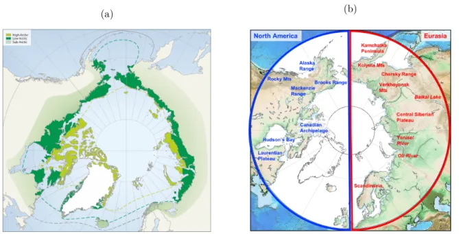
There are several ways to define the Arctic region. The geographical definition is based on solar-Earth motion considering the Arctic as the region above the 66◦340N parallel, the Arctic Circle. When defined in this way, its most fundamental characteristic is continuous daylight during the summer solstice and its absence during winter solstice (polar night). The duration of the daylight hours depends on the latitude. In the extreme case of the North Pole, the sun never sets between spring and autumn equinoxes and never rises during the rest of the year. Another way to set the boundaries of the Arctic is to consider it as the region north of the tree line, where vegetation is mainly dotted shrubs and lichens (Figure 1.1a). Arctic conditions, such as extreme winter cold, widespread permafrost and seasonal snow cover are present south of the limits of the Arctic circle and the tree line delimitation. Therefore, we consider the Arctic domain as the area north of 50◦ latitude and we focused on the ice-free land portion of the Arctic since the aim of this study is to evaluate terrestrial snow characteristics (Figure 1.1b ; see Chapter 3 for further details). Along the Arctic area, for some analysis, we consider separately the North American sector [“NAm”] and the Eurasian sector [“EURA”] separated by the 180◦E meridian (blue and red hemispheres, respectively, in Figure 1.1b ; Table 1.1). Eurasian sector is also split into the Western [“EURAWest”] and the Eastern [“EURAEast”] Eurasian sectors by 90◦E meridian (Table 1.1).

(22)

(a) (b)

Figure 1.1 – (a) Map of high and low Arctic zones delineated according to the Circumpolar Arctic Vegetation Map (CAVM Team 2003). Tree line corresponding to the southern limit of Sub-Arctic zones (extracted from SWIPA (2017)). (b) Arctic domain defined north of 50 degrees latitude (in circle). The terrestrial ice-free Arctic (topographic in color) and the ocean and permanent ice areas (masked in white) are distinguished. Geographical features are labeled to facilitate the spatial description of snow characteristics in the text.

Domain Acronym Longitude

(50◦N − 90◦N)

Arctic ARC 0◦E − 360◦E Eurasia EURA 0◦E − 180◦E Western Eurasia EURAWest 0◦E − 90◦E

Eastern Eurasia EURAEast 90◦E − 180◦E North America NAm 180◦E − 360◦E

Table 1.1 – Arctic domains.

The Arctic climate system is characterized by its low thermal energy state and by its strong couplings between the atmosphere, ocean and land (Serreze and Barry,2014). Arctic encompasses extreme climate differences which varies largely by location and season. Surface air temperature (2 m above ground) presents a marked regional and seasonal variability. The mean temperature of January is less than −35◦C in some parts of Siberia and the Canadian Archipelago, whereas over the central Arctic Ocean, temperature is typically around −25◦C in January (Figure 1.2a). The presence of relatively warm and ice-free ocean water, and the atmospheric heat transport by the North Atlantic cyclones allows Iceland to have a mean temperature in January around 0◦C

(23)

1.1. Arctic climate system 3

(Figure 1.2a). In July, mean temperature over land may vary from 10◦C to 20◦C (Figure 1.2b). Precipitation over the Arctic is quite scarce compare to other regions of the globe. Some parts of the Arctic, such the Canadian Archipelago, can be compared to arid regions elsewhere, with an annual mean precipitation of 200 mm or less ; whereas in the Atlantic sector, where Atlantic cyclones transport the moisture, it can reach 1000 mm (ACIA, 2004; Serreze and Hurst, 2000). Over a considerable part of the terrestrial Arctic, precipitation has maxima in summer but, for the Atlantic sector of the Arctic, maximum occurs in winter due to increase of cyclone activity in the cold season.

Figure 1.2 – Surface air temperature climatology in (a) January and (b) July during 1979-2005 using NCEP/CFSR Reanalysis from ESRL (Earth System Research Laboratory) Monthly/Seasonal Climate Composites https://www.esrl.noaa.gov/psd/cgi-bin/data/composites/printpage.pl .

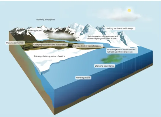
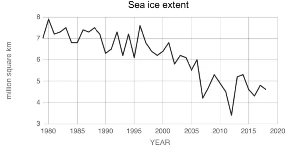
The main feature of the Arctic is its cryosphere, whether sea ice, ice sheets, mountain glaciers and ice caps, permafrost, river and lake ice, and snow (Figure 1.3). The Arctic Ocean occupies most of the surface north of 70◦ latitude and is covered by floating sea ice throughout the year. Summer Arctic sea ice extent has been decreasing since the beginning of the satellite era in the late 70s by -13.3 % per decade (1979-2014) (Serreze and Stroeve, 2015). The alarming record minima of sea ice extent of 4.1 × 106km2 on 14th September 2007 (Comiso et al.,2008) was overtaken on 13th September 2012 reaching 3.4 × 106km2 (Parkinson and Comiso, 2013) (Figure 1.4). Overall, the decline of Arctic annual sea ice extent maximum and minimum has been −2.41 ± 0.56 % per decade and −13.5 ± 2.93 % change relative to the 1979-2015 climate average (Peng and Meier,2018). Sea

(24)

Figure 1.3 – Schematic representation of the components of the Arctic Cryosphere and their associated observed changes caused by global warming (graphic extracted fromSWIPA(2011) and has been adapted from an image created by the U.S. National Center for Atmospheric Research).

ice extent decline is projected to continue during the twenty-first century under different emission scenarios (Collins et al.,2013).

The Greenland ice sheet represents the largest mass of permanent land ice in the Arctic and it has been losing 171 Gt/year in average computed over 1991-2015 (Van den Broeke et al.,2016) with a stronger mass loss of 286 ± 20 Gt/year over the last decade (2010-2018) (Mouginot et al.,2019). Sub-polar ice caps and mountain glaciers are concentrated in the mountainous parts of Siberia and Canadian archipelagos, in Svalbard and Iceland. The monitored Arctic glaciers and ice caps are out of balance with present day climate, which means that they are committed to lose additional mass in the coming decades even if the climate was stabilized in its present state (Mernild et al.,2013). Only 25 ± 35 % of the attributed loss of glacier mass was due to anthropogenic causes during the period from 1851 to 2010, whereas from 1991 to 2010 it has risen to 69 ± 24 % (Marzeion et al., 2014). Permafrost is defined as ground (soil or rock and included ice or organic material) that remains at or below 0◦C for at least two consecutive years (IPA, 2008). It occupies approximately 25% of the Northern Hemisphere land (Biskaborn et al.,2019) and it is also present in sub-sea sediments. Permafrost soils store a large amount of carbon. As temperature increases and permafrost thaws,

(25)

1.2. Snow and climate 5

the carbon contained in permafrost can be released and emitted to the atmosphere as greenhouse gases such as carbon dioxide CO₂ and methane CH₄ (McGuire et al., 2016;Schuur et al., 2015), which in turn increases the pace of future climate change (Schuur et al.,2008).

Figure 1.4 – Time series of annual Arctic sea ice minimum since 1979 to present based on satellite observations. Data from : NSIDC/NASA (https://climate.nasa.gov/vital-signs/arctic-sea-ice/).

1.2 Snow and climate

1.2.1 Snow formation

Snow is crucially important component of the Arctic climate system. Snow originates in cold clouds when two particular conditions are present : supersaturation and supercooling. By definition, an air mass that contains more water vapor than 100% of relative humidity is supersaturated. The higher the temperature, the more water vapor it can hold. As moist air rises, it expands and cools. When supersaturated air cools, the excess of water vapor crystallizes out into water or cloud droplets of the size of ∼10 microns in radius (Armstrong and Brun,2008). When cooled below 0◦C, such small droplets do not necessarily freeze and may “super cool” (i.e. lowering the temperature of gas/liquid below its freezing point without becoming a solid) to a temperature bellow -20◦C and occasionally bellow -40◦C (Armstrong and Brun,2008). Once a droplet has already frozen, it will grow rapidly at the expense of the remaining water droplets as they condense onto the surface of the ice crystal because of the difference in saturation vapor pressure between ice and water. The shape of the initial ice crystal (columnar, platelike, dendritic etc.) depends on the temperature at formation, but

(26)

subsequent growth and structural detail also depend on the degree of saturation (Hobbs,1974). As snow crystals fall down to the ground, they may experience considerable changes since temperature and humidity vary with altitude. The constitution of the surface snow layer depends on the original form of the crystal and the weather conditions during the fall and deposition. Snow on the ground may dissipate quickly through melting or sublimation or may persist for a longer time. In the second case, the snow will undergo metamorphism, changing its grain texture, size, and shape, primarily as a result of temperature and overburden pressure when buried by subsequent snowfalls (Armstrong

and Brun,2008).

Snowpack is described by three basic parameters : snow depth, snow water equivalent (SWE) and snow density. The snow depth is the thickness or the height of snow, usually expressed in cm. The snow water equivalent is the thickness of water resulting from the melting of the initial mass of the snow, which is usually expressed in kg m−2 or mm. Both variables are linked by the snow density, that is the ratio of mass to volume for a given sample, the standard units are kg m−3. For example, considering a maximum seasonal snowpack with a density of ∼ 400 kg m−3 and a height of 50 cm, the resulting SWE will be 200 mm or 200 kg m−2 (see further details in Chapter 2).

1.2.2 Snow properties

Snow is one of the basic elements of the Arctic system, with a duration of snow cover for 7 to 10 months over the year (Figure 1.5) and with a maximum extension of 40% of the Northern Hemisphere land surface (approximately 47 × 106km2) each year (Robinson and Frei,2000;Lemke

et al., 2007). The unique properties of snow have an important impact on climate (Cohen and

Rind,1991;Groisman et al.,1994, ; Figure 1.6). Snow has a strong direct influence on the overlying

low troposphere as has been shown by observations (e.g.,Dewey,1977) and by models (Walsh and

Ross, 1988; Vavrus, 2007) ; the impact is also present in the upper atmosphere (e.g., Alexander

et al., 2010). Snow has high reflectivity and this leads to influence on climate through the

snow-albedo feedback (Qu and Hall,2007;Fletcher et al.,2015), which is a climate feedback mechanism whereby land surface warming is enhanced through reductions in snow cover and surface albedo, and subsequently increased radiation absorbed at the surface (Thackeray et al.,2018). The contribution of terrestrial snow to the Earth radiation budget at the top of the atmosphere through the snow-albedo feedback is nearly equal to that from sea ice, the so-called cryosphere radiative forcing

(27)

1.2. Snow and climate 7

Figure 1.5 – Mean annual snow cover dura-tion over Arctic land areas from the NOAA IMS-24 daily snow cover analysis for the snow sea-sons 1998/99 to 2013/14. Extracted from SWIPA

(2017). The high albedo of snow (0.8-0.9 for dry

snow) together with its low thermal conducti-vity favors low surface air temperatures. This last property is crucial for the insulation of the underlying soil from large energy losses and no-tably for the ice growth rate and the develop-ment of seasonal permafrost (Lawrence and

Sla-ter, 2009; Gouttevin et al.,2012; Koven et al.,

2013;Slater et al.,2017). The impact of snow on

permafrost depends on its duration, thickness, accumulation and melting processes, structure, density, and thermal properties (Zhang et al.,

1996). In summer, late-lying snow cover in-creases surface albedo and thus, surface air tem-perature decreases which prevents permafrost from thawing. In spring, a late snow melt

de-lays warming of the soil surface while it is close to 0◦C, even if the air temperature is positive

(Romanovsky and Osterkamp,1997;Streletskiy et al.,2015). During the snow season, a thick snow

cover insulates the soil from air temperatures below 0◦C which hampers the development of per-mafrost and ice growth. Changes in perper-mafrost temperature are largely attributed to variations on the thickness of snow cover (Streletskiy et al.,2015).Sherstyukov et al.(2008) found that changes in mean annual ground temperature in Siberia are more dependent on snow-cover thickness rather than on changes in air temperature. This relationship has also been found in the Northern Hemis-phere discontinuous zone of permafrost, where ground warming results from the increase of snow thickness, while air temperature remains statistically invariant (Biskaborn et al.,2019).

Snow is a natural store of water, playing a critical role in energy fluxes (release of latent heat), run-off (peak of flow) and evaporation (Groisman et al.,2017). As a natural water reservoir, snow affects the water availability for a substantial part of humanity (Barnett et al.,2005). In the early 1980s,Woostated that the run-off generated by snow in the Arctic drainage basin accounts for 75% of the total annual flow in the Northwest Territories in Canada. Mankin et al. (2015) found that

(28)

the 68 Northern Hemisphere river basins providing water availability to around 2 billion people are exposed to a significant risk of a decrease in snow potential supply in this century.

Figure 1.6 – Schematic illustration outlining the importance of snow on the strong temperature gradients occurring near the snow surface. The solid black line represents an idealized ground-snow-atmosphere temperature profile. Source R. Brown and T. V. Callaghan. Extracted fromCallaghan

et al. (2011b).

1.3 Arctic amplification and its influence on snow

The Arctic has warmed at a pace twice faster than the global average over the past 50 years, a phenomenon known as the Arctic Amplification (Serreze and Barry,2011). Already in 1896, Svante

Arrhenius argued that changes in the concentration of CO2 will influence the global temperature

with a strong impact in polar latitudes. Global warming has a direct impact on the loss of ice cover driving a cascading effect on atmospheric circulation changes (Francis and Skific, 2015; Ma et al.,

2018) as well as on moisture budgets, evaporation and precipitation (Dufour et al.,2016;Liu et al.,

2012;Kattsov and Walsh,2000). However, the inherent complexity of processes involved hinders a

proper understanding of the water cycle feedback (e.g.,Bintanja and Selten,2014) and specifically, the snow response to a changing climate (Brown and Mote,2009;Henderson et al.,2018).

(29)

1.3. Arctic amplification and its influence on snow 9

Arctic warming affects the timing and duration of snow cover, the snow accumulation and

the fraction of precipitation that falls as snow. Snow cover duration is reduced by 2 to 4 days per decade (1972-2014) (Brown et al.,2017) because snow melt occurs earlier in spring (Cayan et al.,

2001;Stewart,2009). This phenomena is not uniform over the whole region : satellite data collected

over the period 1979-2011 have highlighted an averaged reduction of snow cover duration of 1.6 days per decade in the Northern American sector, whereas it reaches 3.3 days per decade in the Eurasian continental sector (Wang et al.,2013). This large reduction of the snow cover season has an immediate impact on the vegetation growth.Barichivich et al. (2013) stated that the Eurasian Arctic has experienced a larger reduction of the vegetation growing season (12.6 days) compared to the North American Arctic region (6.2 days) from 1982 to 2011. As for the snow cover duration, this non-uniform spatial trend distribution has also been observed for other snow characteristics, such as snow depth (Zhong et al., 2018) or snow water equivalent (Mudryk et al., 2015). Using around 820 stations spread all over the Russian Federation during the period from 1966 to 2007,

Bulygina et al. (2009) found that the winter-averaged snow depth decreased in the mountainous

regions of Southern Siberia (− 8-12 cm/dec) ; whereas in the western part of the Russian Federation it increased (around +4-6 cm/dec), with the maximum trends being observed in Northern West Siberia (+8.1 cm/dec at meteorological station Turukhansk at 38 m elevation).Brown et al.(2017) reported a non-significant trend of annual snow depth accumulation of −0.6 cm/dec from 1950 to 2013 in the North American Arctic sector. This trend was computed using 56 stations from the Global Historical Climatology Network (GHCM) which recorded daily snow observations north of 60◦N. Significant decreasing trends in snow depth maximum were found in Yukon and the MacKenzie Basin from 1950 to 2012 ; however, over the rest of the Canadian Arctic, no significant trend could be found (Vincent et al.,2015). Notwithstanding the regional heterogeneities found in the Arctic system, which highlights its complexity, there is multi-dataset evidence that, on average, snow accumulation is decreasing (Brown,2000;Park et al.,2012).

Arctic atmospheric moistening is another consequence of the anthropogenic warming (Min

et al., 2008). The local loss of ice cover (Holland et al., 2007; Bintanja and Selten, 2014) and

the local intensification of water cycle (Rawlins et al., 2010; Dufour et al., 2016) affects Arctic land areas with an increase in precipitation. At midlatitudes with a milder climate, snowfall (solid precipitation) is projected to decrease as the precipitation phase changes to liquid with increasing temperatures ; whereas, in high latitudes with a colder climate, snowfall is projected to increase

(30)

(R¨ais¨anen,2008). The increase in snowfall in deep snowpack regions (i.e. colder regions) may offset the current global reduction in snowfall during a shorter snow season (Wu et al.,2018). In a warmer climate, the timing or amount of snowmelt is associated with a reduction in the peak of stream flow

(Musselman et al.,2017) and an earlier onset of soil moisture drying (Mahanama et al.,2012), as a

larger proportion of snow would melt earlier in the season. The direct consequences are unseasonal thaws (Liston and Hiemstra,2011;Mishra et al.,2010) and an increase of fire risk due to drier soils

(Westerling et al.,2006). Likewise, the decrease in the fraction of precipitation falling as snow leads

to reduced overall stream flow (Berghuijs et al.,2014) and increases the potential for rain-on-snow events (ROS) that even if rare and regional (Cohen et al.,2015) can cause large flooding when they occur (Berghuijs et al.,2016).

1.4 PhD rationale : Snow representation and objectives

The paucity of observational data sets in the Arctic makes it difficult to distinguish with confi-dence the climate forcing signal from the background noise of natural variability in snow evolution

(Brown,2000;Mudryk et al.,2014;Najafi et al.,2016). The spatial distribution of in situ

measu-rements is quite scarce and few long term snow stations exist (Brown and Braaten,1998;Bulygina

et al.,2011). Satellite derived products provide valuable information of snow characteristics (e.g.,

Riggs et al., 2006) but their temporal extent is usually not sufficient for climatological research.

Models are needed to help us to understand snow-related processes, namely, in the context of a warming cryosphere. Land surface models are employed to reproduce the temporal evolution of snow characteristics and its implications for different fields (e.g. hydrology, meteorology, climato-logy, glaciology and ecology). Snow models have been developed with a wide range of complexity. Some models are quite sophisticated with a detailed snow stratigraphy, others with an intermediate degree of complexity using 2-3 layers, and simple, zero-layer (combined with soil) or single layer-snow models (Slater et al.,2001). Generally, in Earth System Models (ESMs), the snow modules are zero- and single-layer configurations. These simple models require fewer parameterizations, leading to faster computation ; however, they experience some limitations (Bokhorst et al., 2016;Krinner

et al.,2018).

In this research we focus on the evaluation of General Circulation Models (GCMs) from the Coupled Model Intercomparison Project 5 (CMIP5). CMIP5 is a standard framework from the World Climate Research Program (WRCP) aiming at improving our collective knowledge about

(31)

1.4. PhD rationale : Snow representation and objectives 11

the climate system. Currently, there have already been many studies evaluating the GCMs from the CMIP5 project (Flato et al., 2013). Our work builds upon previous studies assessing snow characteristics in general circulation models where some progress and faults have been identified

(Flato et al.,2013;Brutel-Vuilmet et al.,2013;Kapnick and Delworth,2013;Terzago et al.,2014).

One of the main results was that the observed decreasing trend in spring snow cover in the Northern Hemisphere over the period 1979-2015 (Derksen and Brown, 2012) is largely underestimated in CMIP5 models due to an underestimation of the boreal temperature (Brutel-Vuilmet et al.,2013). Also, the spread in snow-albedo feedback (SAF) was not reduced from CMIP3 likely due to a wide spread in the different treatment of vegetation in models (Qu and Hall,2013). Recently,Thackeray

et al. (2018) found that indeed, the structural differences in the snowpack, vegetation and albedo

parametrizations drive most of the spread. Notably, models displaying the largest bias in SAF, also show clear structural and parametric errors. However, snow regimes in autumn have received less attention compared to spring.

In this respect, representation of snow-associated feedbacks in climate models, especially during the mid seasons (when Arctic snow cover exhibits the strongest variability) is of a special interest. At the offset of the snow season, down-welling shortwave and longwave radiation fluxes provide most of the energy enabling snow melt ; at the onset, temperatures are sufficiently cold to favor solid precipitation and snow accumulation (Sicart et al.,2006). In spring, the snow albedo feedback is stronger as snow cover starts to age and recede due to increasing temperature and insolation (Qu

and Hall, 2013; Thackeray et al., 2016). In addition, positive (negative) snow cover anomalies in

Eurasia from winter to spring may be followed by negative (positive) anomalies in the rainfall during the Indian summer moonson (Prabhu et al.,2017;Senan et al.,2016) but this snow-teleconnection is still controversial (Peings and Douville, 2010; Zhang et al., 2019). While variations in snow characteristics are smaller in autumn than in spring, they also experience changes which have links to atmospheric circulation (Henderson et al.,2018). Observational (Cohen et al.,2007) and modeling

(Peings et al.,2012) studies linked the increase in Eurasian snow cover with the winter phase of the

Arctic Oscillation (AO) and North Atlantic Oscillation (NAO). However, Gastineau et al. (2017) using an ensemble of CMIP5 models, demonstrated that this relationship is simulated by only four models and is largely underestimated by the majority of the ensemble.Douville et al. (2017) have questioned the robustness of the snow-NAO relationship and also argued for the importance of eastward phases of the Quasi-Biennial Oscillation (QBO) in modulation of snow cover variability.

(32)

To summarize, there is a need for comprehensive evaluation and validation of snow characte-ristics in climate models using available observations over the last decades in order to demonstrate which Arctic snow features are more robust across different models and which are not captured effectively. The focus of this PhD is on the representation of Arctic terrestrial snow in global circu-lation models from the CMIP5 ensemble in the mid seasons. Our goal is to make an evaluation of individual models to provide reliable information for the scientific community and hopefully help to improve the snow representation in future general circulation models. This thesis is organized as follows. Chapter 2 describes the snow data sources –namely, CMIP5 models, reanalyses and observations. Chapter 3 is dedicated to the description of the methodology, the treatment of data to provide comparability and the statistical tools employed. Chapter 4 presents the analysis of the spatial structure of snow characteristics. In Chapter 5 we study the temporal evolution and varia-bility of snow characteristics. Finally, Chapter 6 offers the main conclusions and some perspectives for future research.

(33)

Chapter 2

Data

Contents

2.1 Overview . . . . 13

2.2 General Circulation Models (GCMs) . . . . 14

2.2.1 Coupled Model Intercomparison Project 5 : CMIP5 . . . 14

2.2.2 Snow Variables in CMIP5 . . . 19

2.3 Observations . . . . 22

2.3.1 Snow Stations . . . 23

2.3.2 NOAA CDR . . . 23

2.3.3 CanSISE Ensemble Product . . . 24

2.3.4 Reanalyses . . . 25

2.1 Overview

Our capacity to observe the terrestrial Arctic is limited compared to the mid-latitudes. Condi-tions are not ideal for continuous monitoring of snow characteristics due to inclement weather conditions, the polar night and the wind transport of snow. Moreover, the uneven spatial distribu-tion of snow stadistribu-tions concentrated at 55◦N in Canada (Brown and Braaten, 1998) or the lack of data in northern Siberia (Bulygina et al.,2011) make challenging the up-scaling to larger regions. The snow stations are key for climatological research of snow characteristics as they are a unique record and the longest existing data in time. The temporal extent of the satellite era usually limits the study of the climate variability of snow (Maurer et al.,2003;Riggs et al.,2006). Even if both the in situ measurement and satellite data provide valuable information for snow and environment

(Groisman and Davies,2001), they present the aforementioned spatial and temporal limitations.

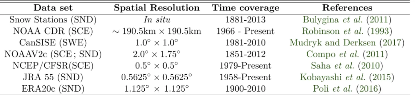
Reanalyses are a combination of observations and numerical models proving a synthesized es-timate of the Earth system. They can reproduce the state of the climate and extend over several decades, as is the case for the NCEP/CFSR (Saha et al.,2010) and ERA-Interim (Dee et al.,2011) reanalyses ; or longer time periods, as the NOAA-CIRES 20th reanalysis (Compo et al.,2011). Ty-pically, reanalysis products cover the entire globe from the surface to well above the stratosphere.

(34)

Land snow-cover models are used to simulate the temporal evolution of snow in multiple ap-plications (e.g. hydrology, meteorology, climatology, glaciology and ecology). There exist a wide variety of empirical and physically-based snow models whose degree of complexity may be adjusted to the intended application (Magnusson et al., 2015). The sophistication of snow models ranges from the more complex with a detailed snow stratigraphy (e.g., CROCUS ;Brun et al.,1992,1997;

Vionnet et al., 2012), i.e vertical evolution of snow properties like snowpack compaction, liquid

water percolation, snow interception etc., through the intermediate model complexity (2-3 layers) and to the simplest, with zero-layer (combined with soil) or single layer-snow models (Slater et al.,

2001). The modules used in Earth System Models (ESMs) are usually zero- and single-layer snow model configurations, having fewer parameterizations leading to fast computations, however, they involve some limitations (Bokhorst et al., 2016; Krinner et al., 2018). Some of the flaws in ESMs have been linked to the representation of the vegetation (Essery, 2013; Thackeray et al., 2015), thermal conductivity (Cook et al.,2008;Gouttevin et al.,2012) and radiative processes (Thackeray

et al., 2016). However, even in detailed physically-based models, there are snow related processes

that are not well captured, particularly in cold conditions (Domine et al., 2016). The uncertainty of the underlying physics remains a drawback in the advance of snow modeling (Lafaysse et al.,

2017).

This chapter describes the wide variety of data used, from general circulation models to snow stations through the different satellite-based products and reanalyses, in order to bridge the gaps between the representations of snow characteristics in such a variety of data sets.

2.2 General Circulation Models (GCMs)

2.2.1 Coupled Model Intercomparison Project 5 : CMIP5

As a part of the World Climate Research Program (WCRP), CMIP5 (Taylor et al.,2012, Cou-pled Model Intercomparison Project Phase 5) is a standard framework for studying the output of coupled atmosphere-ocean general circulation models (“AOGCMs”). CMIP5 builds on the accom-plishment of previous CMIP phases (Meehl et al.,2000,2005) and aims at advancing our collective understanding of climate variability and climate change. The CMIP5 framework includes simu-lations on several timescales, ranging from seasonal to multidecadal. All simusimu-lations included in the CMIP5 framework (Figure 2.1) are classified by “core” and by one or two surrounding “tiers”

(35)

2.2. General Circulation Models (GCMs) 15

according to a consensus of prioritization. The “core” simulations (shaded in pink, Figure 2.1) are crucial for the evaluation of climate models and they produce information of keen interest about future projections. The “tier1” (shaded in yellow, Figure 2.1) researches specific aspects of climate model forcing, responses and processes that are examined in further depth in “tier2” (shaded in green, Figure 2.1). The strategy of CMIP5 encompasses two type of climate experiments (Figure 2.1a,b) that we briefly describe below :

1. Long-term integrations (century time scale) (Figure 2.1a) are usually started from mul-ticentury preindustrial control (quasi equilibrium). These simulations follow the protocol of the previous phases of CMIP, but they add some additional runs to supply a more exhaustive understanding of climate change and variability. The core of long-term simulations (Figure 2.1a) involve an AMIP run, a coupled control run and a “historical” run. The latter are forced by observed atmospheric composition and reflect both the anthropogenic and the natural evo-lution of the climate system. The historical runs, also called “twentieth century” simulations, cover the time period from 1850 to 2005. The new addition with respect to previous phases is that in CMIP5, the historical runs include a time-evolving land cover.

Within the long-term simulations, there are also future projections forced with specified concentrations of greenhouse gases, which are referred to as “representative concentration pathways” (RCPs) described in Moss et al. (2010). In CMIP5, there are four RCPs which are based on estimations of future population growth, technological development and societal responses (Figure 2.2). The denomination of each RCP provides an approximate estimate of the radiative forcing in the year 2100 (relative to preindustrial conditions). Unlike phase 3, in CMIP5, these RCPs take policy interventions into account, meaning that the RCPs are mitigation scenarios where actions to curb emissions are considered. The four future scenarios are : RCP8.5, referred to as the “high scenario”, the two “intermediate scenarios” RCP4.5 and RCP6, and the so called “peak-and-decay” scenario RCP2.6.

2. Near-term integrations (10-30 yr) (Figure 2.1b), also called decadal prediction expe-riments (Meehl et al., 2009). The near-term prediction experiments are a novelty of CMIP. Decadal prediction experiments are organized by the WGCM and the Working Group on Sea-sonal to Interannual Prediction (WGSIP). These near-term simulations are initialized with observed ocean and sea ice conditions. There are two collections of core simulations (Figure

(36)

(a) (b)

Figure 2.1 – (a) Schematic summary of CMIP5 long-term experiments. Upper hemisphere expe-riments are suitable for validation with observations or provide projections. Green fonts refer to simulations performed only by models with carbon cycle representations. (b) Schematic summary of CMIP5 decadal prediction integrations. Extracted from Taylor et al.(2012).

2.1b) : i) a set of 10 year hindcasts initialized from observed climate states near every five years from 1960 to 2005 ; ii) two 30-year hindcasts initialized in 1960 and 1980, and one 30 year prediction initialized in 2005, ending in 2035. In the first one, we can asses the skill of the climate forecast when initial climate conditions exert some detectable influence, whereas in the second one, with a longer time scale, the external forcing of an increase in GHGs will dominate the response of the system even if some residual influence of the difference in ini-tial conditions prevail. Thus, in the near-term simulations models are not only responding to climate forcing (e.g. increase in CO₂ concentration) but they may also reproduce the climate change evolution, including the unforced component.

Climate models involved in CMIP5 have a twofold mission. First, purely scientific, aims at advancing in our knowledge of the Earth Climate System, its past, present and future evolution. The second is to contribute to the IPCC (Intergovernmental Panel on Climate Change) reports to mitigate climate change and adapt to its effects (Edenhofer et al.,2014;Field et al.,2014).

(37)

Figure 2.2 – Time series of compatible emission rate (PgC yr−1) of fossil fuel emissions simulated by the CMIP5 ESMs for the four RCP scenarios. Dashed lines represent the historical estimates and emissions calculated by the Integrated Assessment Models (IAMs) used to define the RCP scenarios ; solid lines and shading show results from CMIP5 ESMs (model mean, with 1 standard deviation shaded). Extracted from Ciais et al. (2014).

The straightforward approach to model evaluation is to compare the model output with existing observations to identify its strengths and weaknesses. The core of this PhD is to contribute to this vast task by analyzing the snow characteristics in CMIP5 models. For this purpose, we evaluate the most realistic simulations from CMIP5, the “historical runs” from the “long-term integration” type climate experiments. They are forced by observed atmospheric composition and exhibit the anthropogenic forcing as well as the natural evolution of the climate system.

(38)

Mo del name Mo deling Cen ter (Institut ID) Resolution Nb mem b ers Reference b cc-csm1-1 Beijing Cli mate Cen ter, China Meteorological A dministra-tion (BCC) 2 .8 ◦ × 2 .8 ◦ 3 W u et al. ( 2013 ) CanESM2 Canadian Cen ter for Climate Mo deling and Analysis (CCCMA) 2 .8 ◦ × 2 .8 ◦ 5 Arora et al. ( 2011 ) CCSM4 National Cen ter for A tmosph e ric Researc h (NCAR) 0 .9 ◦ × 1 .2 ◦ 8 Gen t et al. ( 2011 ) CNRM-CM5 Cen tre National de Rec h e rc hes M ét éorologiques/Cen tre E u-rop éen de Rec herc he et F ormation A v anc ée en Calcul Scien-tifique (CNRM-CERF A CS) 1 .4 ◦ × 1 .4 ◦ 10 V oldoire et al. ( 2012 ) CSIR O-Mk3-6-0 Common w e alth Scien tific and Industrial Researc h Organiza-tion in collab oration with Queensland Climate Change Cen-ter of Excelle n c e (CSIR O-QCCCE) 1 .8 ◦ × 1 .8 ◦ 10 Collier et al. ( 2011 ) GISS-E2-H NASA Go ddard Institute for Space Studies (NASA GISS) 2 .0 ◦ × 2 .5 ◦ 6 Sc hmidt et al. ( 2006 ) GISS-E2-R 6 Sc hmidt et al. ( 2006 ) inmcm4 Institute for Numerical Mathematics (INM) 1 .5 ◦× 2 .0 ◦ 1 V olo din et al. ( 2010 ) MIR OC-ESM-CHEM Japan Agency for Marine-Earth Scie n c e and T ec hnology , A t-mosphere and Ocean Re se arc h Institute (The Univ ersit y of T oky o), and National Institute for En vironmen tal Studies (MIR OC) 2 .8 ◦ × 2 .8 ◦ 1 W atanab e et al. ( 2011 ) MIR OC-ESM 2 .8 ◦ × 2 .8 ◦ 3 W atanab e et al. ( 2011 ) MIR OC5 1 .4 ◦ × 1 .4 ◦ 5 W atanab e et al. ( 2010 ) MPI-ESM-LR Max Planc k Institute for Meteorology (MPI-M) 1 .8 ◦ × 1 .8 ◦ 3 Giorgetta et al. ( 2013 ) MPI-ESM-P 2 Giorgetta et al. ( 2013 ) MRI-CGCM3 Meteorological Researc h Institute (MRI) 1 .1 ◦ × 1 .1 ◦ 5 Y ukimoto et al. ( 2012 ) NorESM1-M Norw egian Cl imate Cen ter (NCC) 1 .8 ◦ × 2 .5 ◦ 3 Ben tsen et al. ( 2013 ) NorESM1-ME 2 Ben tsen et al. ( 2013 ) T abl e 2.1 – CMIP5 mo dels, mo deling ce n ter and institute acron ym (h ttps://cmip.llnl.go v/cmip5/ ), resolution and n um b er of ensem ble mem b ers considered.

(39)

2.2.2 Snow Variables in CMIP5

In the introduction it was mentioned that the snowpack can be described by snow depth or snow water equivalent, and that both characteristics are related by the snow density. From the in situ point of view, snow depth usually refers to the total height of snow on the ground at the time of observation and it is measured with a snow ruler or similar graduated rod which is pushed down through the snow to the ground surface (Jarraud,2008). Snow water equivalent is the thickness of the water that would be obtained by melting the snow sample and it can be measured directly by melting the sample and measuring its liquid content, or indirectly by inferring the water equivalent using an appropriate specific snow density (Jarraud, 2008). Returning to the example from the introduction, for a snow sample of 50 cm height with a maximum seasonal snow density of 400 kg m−3, the resulting snow water equivalent would be 200 mm following this relationship :

mliquid water = msnow

ρliquid water· hliquid water· S = ρsnow· hsnow· S

→ h_{liquid water} = ρsnow=400 kg m−3

ρ_{liquid water=1000 kg m−3} · hsnow=0.5 m= 200 mm

However, when moving from the in situ representation to large scale, the concept of snow cha-racteristics is slightly nuanced. From the model perspective, there is no one observation point ; instead, space is discretized in grid cells which makes the conversion of snow depth to snow water equivalent much more complex. Indeed, in CMIP5 models, the spatial resolution of grid cells varies from ∼ 100 km2 to ∼ 300 km2. The snow surface representation also depends on the different cano-pies within the grid cells, that is, the type of vegetation (e.g. trees, shrubs), topography, land use, presence of lakes and rivers etc. which are in the land-surface model of the GCM. The variables that represent terrestrial snow characteristics in CMIP5 models are described in the document “standard output.pdf” accessible via https://pcmdi.llnl.gov/mips/cmip5/docs/ :

• Snow Area Fraction (“snc”, %) : Fraction of each grid cell that is occupied by snow that rests on the land portion of the cell. “Snow Area Fraction” is usually called “Snow Cover Extent” ; throughout the manuscript we will refer it as “SCE”.

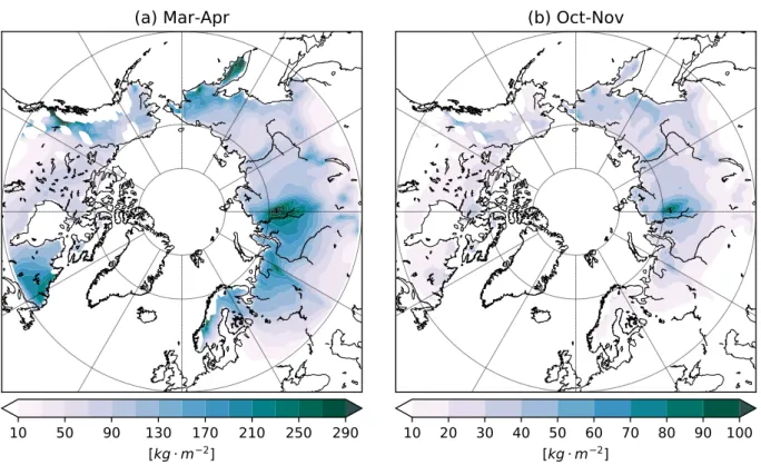
• Surface Snow Amount (“snw”, kg m−2_{) : Computed as the mass of surface snow on the}

land portion of the grid cell divided by the land area in the grid cell ; reported as 0.0 where the land fraction is 0 ; snow on vegetation canopy or on sea ice is excluded. “Surface Snow

(40)

Amount” corresponds to the snow water equivalent definition (hw in Figure 2.3) ; hereafter

we will refer to it as “SWE”.

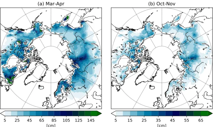
• Snow Depth (“snd”, m) : when over land, this is computed as the mean thickness of snow in the land portion of the grid cell (averaging over the entire land portion, including the snow-free fraction). Reported as 0.0 where the land fraction is 0. Snow depth (“SND”) is represented by hsnow as in Figure 2.3.

Figure 2.3 – Diagram of snow characteristics in general circulation models.

In the CMIP5 models considered in this study (Table 2.1), the snow water equivalent (SWE) is a prognostic variable (ES-DOC, https://es-doc.org) resulting from the balance between snowfall, evaporation and snowmelt rates (Equation 2.1 ;Manabe,1969;Thackeray et al.,2016). Snow depth (SND) is usually a diagnostic variable depending on SWE by means of the snow density.

d

dt(SW E) = Sf − E − Me (2.1)

where S_f is the rate of snowfall, E is the evaporation rate and M_eis the rate of snow melt which can be computed by the heat balance (E_x) condition of a snow covered surface, that is, M_e = E_x/Lf

when E_x > 0 and Me = 0 when Ex <= 0 (Manabe, 1969). Snow cover fraction or extent (SCE)

is usually diagnosed from SWE by means of a monotonic function using different parametrizations depending on the model (Liston,2004;Wu et al.,2018). Models also present different conservation

(41)

properties (e.g. water discharge-storage), couplings with atmosphere and land cover types which depend essentially on the land model integrated in the GCM. For example, to diagnose SCE, the ISBA surface model, a component of CNRM-CM5, uses an asymptotic function of SWE (Equation 2.2 ; Douville et al.,1995) :

png=

Wn

Wn+ Wcrn(= 10mm)

(2.2)

where Wn is the mean snow water equivalent (SWE), Wcrn the critical water equivalent of snow

necessary to the estimation of png which represents the fraction of snow covering the soil (SCE)

(Douville et al.,1995). Conversely, the CLM 3.5 land model from CCSM4 uses a tangential

hyper-bolic function (Equation 2.3 ;Niu and Yang,2007;Xu and Dirmeyer,2013).

SCE = tanh " hsnow αz0g(ρsnow/ρnew)β # (2.3)

where hsnowis the spatially averaged snow depth (expressed as a function of SWE and snow density),

and z0g is the surface roughness length. The ρsnow is the model-calculated snow density and ρnew

is a prescribed fresh snow density of 100 kg m−3, β is a tunable parameter depending on several factors (e.g. vegetation, orography) and α is fixed to 2.5 for simplicity in the global model (Xu and

Dirmeyer,2013).

CMIP5 Snow Data Archive In order to facilitate the model output, the CMOR2 software library was created where variables are stored following this standard filename format (https:// cmip.llnl.gov/cmip5/docs/CMIP5 output metadata requirements.pdf,Taylor et al.,2011) :

filename = <variable name> <MIP table> <model> <experiment> <ensemble member> <temporal subset>].nc

The snow land variables such as SCE, SWE and SND are stored as “Monthly Mean Land Cryosphere Fields” with the corresponding filename encoding :

snow filename = snow LImon <model> historical <ensemble member> <period>.nc The <MIP table> provides information about the modeling realm, the high level modeling component relevant for the variable such as “LandIce” for snow or “Atmosphere” for snowfall, and also the frequency, “Monthly” in both cases. The experiment family is indicated as “historical”, referring to the historical runs explained in the previous section. The ensemble member is

(42)

com-posed by a triad of integers (r<N>i<M>p<L>) which refer to varying simulation conditions for each realization (member). N is the “realization number ” : if the different members of one model vary only according to this integer N, it means that runs have been initialized with different, but equally realistic initial conditions ; the M corresponds to the “initialization method indicator ” which indicates the different observational data sets or the different methods using observations that are employed as initial conditions. The L refers to the “perturbed physics number ” which allows to distinguish between different realizations that have modified a particular set of model parameters. The <temporal subset> is restricted to the period 1979-2005.

The choice of the ensemble of models in Table 2.1 is justified by two reasons. First, our aim was to evaluate different snow variables and so, initially, we only focused on snow cover and snow water equivalent (SCE and SWE). Thus, we considered only the CMIP5 models which provided both characteristics. Later in the PhD, we began to use in situ measurements from the snow stations, which motivated us to form a new set of models including snow depth ; however, the models MPI-ESM-LR/P do not provide this variable. The risk of using an erroneous method to convert SWE to SND to include these models in the SND analysis has already been identified (Brown and Frei,

2007). Consequently, in the SND analysis the MPI-ESM-LR/P models do not appear. Secondly, we wanted to limit our study to an amount of models small enough to enable individual analysis. When using a large number of models, multimodel analysis is more suitable, but it is less evident to provide a catalog of individual model performance.

2.3 Observations

Generally, there are two fundamental ways to measure snow directly, from in situ snow stations and from remote sensing using satellites (e.g.,Riggs et al.,2006) or airborne LiDAR (e.g.,

Schaff-hauser et al., 2008). The main problem with in situ measurements is that they include intrinsic

systematic human error (Woo and Marsh,1978) and may not be accurately continuous in time. On the other hand, they are a unique record with precious information of snow characteristics. Remote sensing snow data coming from satellites, for instance, contain uncertainties related to the retrieval procedure such as the presence of clouds (Parajka and Bl¨oschl,2006). They are continuous in time, however, satellite snow products begin too late for our period of interest, except for the NOAA Climate Data Record (Estilow et al.,2015). Reanalysis products are another source of snow

(43)

infor-2.3. Observations 23

mation considered here as an observational reference. However, they are also subject to intrinsic errors (e.g.,Khan et al.,2008;Dufour et al.,2016;Wegmann et al.,2017).

2.3.1 Snow Stations

Regular snow observations have been conducted all over the Eurasian continent from 1881 to 2013. This includes snow depth measurements and the amount of snow covering the visible area of meteorological stations, estimated on a scale of one to ten (10 to 100% ; or zero in the absence of snow). Here we use the daily snow depth record over the former USSR (Union of Soviet Socialist Republics), which is composed of data from 600 stations, from the Russian Research Institute for Hydro-meteorological Information - World Data Center (RIHMI-WDC) (Bulygina et al., 2011). Snow depth measurements have been conducted once a day using a graduated stake installed at a fixed point location within the station or by a wooden ruler, following the standard protocol from the World Meteorological Organization (WMO, McMichael et al., 1996). Meteorological data sets are quality controlled before being stored at the RIHMI-WDC (Veselov,2002). As the procedures of snow observation have changed over time (e.g.,Meshcherskaya et al.,1995), particular consideration has been taken to maintain the homogeneity in the data record. All information for the snow stations is available at http://meteo.ru/english/climate/snow.php.

2.3.2 NOAA CDR

The satellite-based weekly Snow Cover Extent dataset (Robinson et al., 1993; Robinson and

Frei, 2000;Estilow et al., 2015) is the longest continuous record of snow cover extent, starting on

4th October 1966 and continuing at present. It is freely available at the NOAA (National Oceanic and Atmospheric Administration) National Center for Environmental Information (NCEI). It has been used in numerous studies (D´ery and Brown, 2007; Derksen and Brown, 2012; Brown and

Derksen,2013;Gastineau et al.,2017;Connolly et al.,2019). Before 1972, the resolution of common

meteorological satellites was around 4 km. From October 1972, VHRR (Very High Resolution Radiometer) provided imagery with an improved spatial resolution of 1 km, which was slightly reduced to 1.1 km in November 1978 with the replacement of the VHRR by the Advanced VHRR (AVHRR). From 1966 to 1999, snow maps were analyzed and interpreted by hand by experienced meteorologists from the NOAA who drew the boundaries of snow cover extension. Weekly maps were created in an 89 × 89 cell cartesian grid laid over a polar stereographic projection of the