Development of origin–destination
matrices using mobile phone call data
The MIT Faculty has made this article openly available. Please share how this access benefits you. Your story matters.Citation Iqbal, Md. Shahadat; Choudhury, Charisma F.; Wang, Pu and González, Marta C. “Development of Origin–destination Matrices Using Mobile Phone Call Data.” Transportation Research Part C: Emerging Technologies 40 (March 2014): 63–74. © 2014 Elsevier Ltd
As Published http://dx.doi.org/10.1016/j.trc.2014.01.002
Publisher Elsevier
Version Author's final manuscript
Citable link http://hdl.handle.net/1721.1/108682
Terms of Use Creative Commons Attribution-NonCommercial-NoDerivs License
1 2
Development of Origin-Destination Matrices Using Mobile Phone Call Data:
3
A Simulation Based Approach
4 5
Md. Shahadat Iqbal 6
Department of Civil Engineering. 7
Bangladesh University of Engineering and Technology, Dhaka 1000, Bangladesh 8 [email protected] 9 10 11 Charisma F. Choudhury* 12
Institute for Transport Studies 13
University of Leeds, Leeds LS2 9BJ, UK 14 [email protected] 15 16 Pu Wang 17
School of Traffic and Transportation Engineering 18
Central South University, Hunan 410000, P.R. China 19
20 21
Marta C. Gonza´lez 22
Department of Civil and Environmental Engineering, 23
Massachusetts Institute of Technology, Cambridge, MA 02139, USA 24 25 26 27 28 29 30 31
Word Count Tables and Figures 13 x 250 = 3250
32 Word Count 3814 33 Total 7064 34 35 36 37 38 39 40 41 *Corresponding Author 42
Abstract
43
In this research, we propose a methodology to develop OD matrices using mobile phone Call
44
Detail Records (CDR), which consist of time stamped tower locations with caller IDs, and
45
limited traffic counts. CDR from 2.87 million users from Dhaka, Bangladesh over a month and
46
traffic counts from 13 key locations of the city over 3 days of the same period are used in this
47
regard. The individual movement patterns within certain time windows are extracted first from
48
CDR to generate tower-to-tower transient OD matrices. These are then associated with
49
corresponding nodes of the traffic network and used as seed-OD matrices in a microscopic traffic
50
simulator. An optimization based approach, which aims to minimize the differences between
51
observed and simulated traffic counts at selected locations, is deployed to determine scaling
52
factors and the actual OD matrix is derived. The applicability of the methodology is supported by
53
a validation study.
54 55
Keywords: Mobile phone, Origin-Destination, Video Count, Traffic Microsimulation
1. Background
57
Reliable Origin-Destination (OD) matrices are critical inputs for analyzing transportation
58
initiatives. Traditional approaches of developing OD matrices rely on roadside and household
59
surveys, and/or traffic counts. The roadside and household surveys for origin destination involve
60
expensive data collection and thereby have limited sample sizes and lower update frequencies.
61
Moreover, they are prone to sampling biases and reporting errors (e.g.1,2,3). Estimation of
62
reliable OD matrices from traffic link count data on the other hand is extremely challenging
63
since very often the data is limited in extent and can lead to multiple plausible non-unique OD
64
matrices (4,5). A number of Bayesian methods (e.g.6,7,8), Generalized Least Squares approaches
65
(e.g.9,10), Maximum Likelihood Approaches (11), and Correlation Methods (e.g.12,13,14) have
66
been used to tackle the indeterminacy problem. These approaches typically use target matrices
67
based on prior information for generating the plausible route flows and are very sensitive to this
68
prior information as well as to the chosen methodology (15). More recent approaches for OD
69
estimation include automated registration plate scanners (16) and mobile traffic sensors such as
70
portable GPS devices (e.g.17,18,19) . The practical successes of these approaches have however
71
been limited due to high installation costs of the license plate readers and the low penetration
72
rates of GPS devices (especially in developing countries). 73
Mobile phone users on the other hand also leave footprints of their approximate locations
74
whenever they make a call or send an SMS. Over the last decade, mobile phone penetration rates
75
have increased manifold both in developed and developing countries: the current penetration
76
rates being 128% and 89% in developed and developing countries respectively (20).
77
Subsequently, mobile phone data has emerged as a very promising source of data for
78
transportation researchers. In recent years, mobile phone data have been used for human travel
79
pattern visualization (e.g. 21,22,23), mobility pattern extraction (e.g. 24,25,26,27,28,29), route
80
choice modeling (e.g. 30,31), traffic model calibration (e.g. 32), traffic flow estimation (33) to
81
name a few. There have been several limited scale researches to explore the feasibility of
82
application of mobile phone data for OD estimation as well. Wang et al. (34) for instance use a
83
correlation based approach to dynamically update a prior OD matrix using time difference of
84
phone signal receipt times of base stations and Caceras et al. (35) use a GSM network simulator
85
to simulate the detailed movements of phones that are turned on. But both of these feasibility
86
studies are based on synthetic data in small networks and the practical application is challenging
87
given the need to collect and process detailed location data (which are currently processed by the
88
mobile phone companies for load management purposes but are not stored). The potential
89
estimate OD matrices using mobile phone Call Detail Records (CDR) (which are stored by
90
operators for billing purposes and hence more readily available) have also been explored (e.g.
91
36,37,38). Mellegård et al. (36) have developed an algorithm to assign mobile phone towers
92
extracted from CDR to traffic nodes and Calabrese et al. (37) have proposed a methodology to
93
reduce the noise in the CDR data but both studies have focused more on computation issues and
94
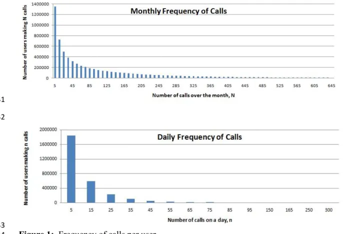
the relationship between the mobile phone OD and the traffic OD have not been explored in
detail. Wang et al. (38) have used an analytical model to scale up the ODs derived from CDR by
96
using the population, mode choice probabilities and vehicle occupancy and usage ratios and have
97
validated it using probe vehicle data. The methodology however relies heavily on availability of
98
traffic and demographic data in high spatial resolution which may not be always available,
99
particularly in developing countries.
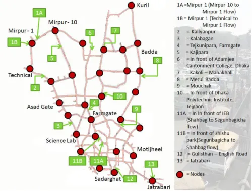
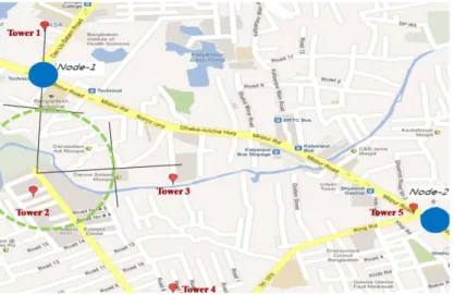
100
In this research, we propose a methodology to develop OD matrices using mobile phone CDR
101
and limited traffic counts. CDR from 2.87 million users from Dhaka, Bangladesh over a month
102
are used to generate the OD patterns on different time periods and traffic counts from 13 key
103
locations of the city over a limited time are used to scale it up to derive the actual ODs using a
104
microscopic traffic simulator. The methodology is particularly useful in situations when there is
105
limited availability of high resolution traffic and demographic data. The ODs are validated by
106
comparing the simulated and observed traffic counts of a different location (which has not been
107
used for calibration).
108
The rest of the paper is organized as follows. First we describe the data followed by the
109
methodology used for development of the OD matrix. The estimation and validation results are
110
presented next. We conclude with the summary of findings and directions for future research.
111
2. Data
112
2.1 Study Area
113
The central part of the Dhaka city has been selected as the study area and the major roads in the
114
network has been coded. This consists of 67 nodes and 215 links covering an area of about
115
300km2 with a population of about 10.7million (39). The average trip production rate is 2.74 per
116
person per day with significant portions of walking (19.8%) and non-motorized transport trips
117
(38.3%) (39).The traffic is subjected to severe congestion in most parts of the day, the average
118
speed being only 17km/hr1.
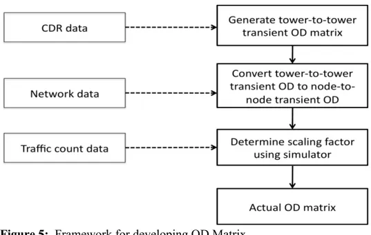
119
The mobile phone penetration rate is approximated to be more than 90% in Dhaka (66.36%
120
being the national average) and Grameenphone Ltd. has the highest market share with 42.7m
121
mobile phone subscribers nationwide (40).
122
2.2 CDR Data
123
The CDR data, collected from Grameenphone Ltd, consists of calls from 6.9 million users
124
(which are more than 65% of the population of the study area) over a month. This comprises of
125
971.33 million anonymized call records in total made in between June 19, 2012 and July 18,
126
2012. The majority of the users (63%) have made 100 calls or less over the month. The
127
frequencies of users making certain number of calls over the month and on a randomly selected
128
day (15th July, 2012) are presented in Figure 1. It may be noted that no demographic data related
129
to the phone users are available.
130
131 132
133
Figure 1: Frequency of calls per user
134
2.3 Traffic Count Data
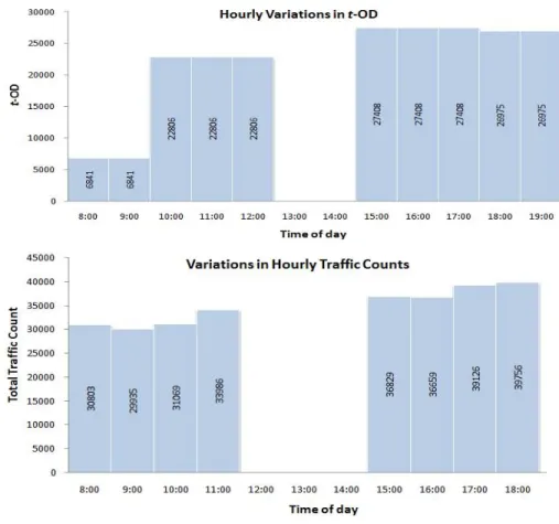
135
Video data, collected from 13 key locations of Dhaka city network over 3 days (12th, 15th and
136
17th July 2012) have been used in this study to extract the traffic counts2. The locations (shown
137
in Figure 2) have been selected such that they cover the major roads (links) of Dhaka city with
138
flows from major generators and governed by the availability of foot over bridges for mounting
139
video cameras. Since MITSIMLab is developed for lane-based motorized traffic, care has been
140
taken to avoid roads that have high percentages of non-motorized transport and where
lane-141
discipline is not strictly followed. The data has been collected for 8 hrs (8.00 am to 12.00 noon
142
and 3.00 pm to 7.00pm) and analyzed using the software TRAZER (41) to generate classified
143
vehicle counts. Due to inclement weather and poor visibility some portion of the data is
non-144
usable though. Moreover, TRAZER (which is the only commercial software that can deal with
145
mixed traffic streams with ‘weak’ lane discipline) has high misspecification rates in presence of
146
high congestion levels and in those cases, manual counting has been performed instead.
147 148
149
150
Figure 2: Locations of video data collection and position of OD generating nodes
151
3. Methodology
152
Each entry in the CDR contains unique caller id (anonymized), the date and time of the call, call
153
duration and latitude and longitude of the Base Transceiver Station (BTS). A snapshot of the data
154
is presented in Figure 1. As seen in the figure, if a person traverses within the city boundary and
155
uses his/her phone from different locations that is captured in the CDR. CDR can thus provide an
156
abstraction of his/her physical displacements over time (Figure 3).
157
ID Call Date Call Time Duration Latitude Longitude
AH03JAC8AAAbXtAId 20120701 09:34:19 18 23.8153 90.4181 AAH03JABiAAJKnPAa5 20120707 06:15:20 109 23.8139 90.3986 AAH03JABiAAJKnPAa5 20120707 09:03:06 109 23.7042 90.4297 AAH03JABiAAJKnPAa5 20120707 10:34:19 16 23.6989 90.4353 AAH03JABiAAJKnPAa5 20120707 18:44:53 154 23.6989 90.4353 AAH03JABiAAJKnPAa5 20120707 20:00:08 154 23.8092 90.4089 AAH03JAC5AAAdAYAE 20120701 09:15:05 62 23.7428 90.4164 AAH03JAC+AAAcVKAC 20120707 08:56:34 242 23.7908 90.3753 AAH03JAC+AAAcVKAC 20120701 18:03:06 36 23.9300 90.2794 AAH03JAC5AAAdAYAA 20120701 11:15:55 12 23.7428 90.4164 158
Figure 3: An excerpt from CDR data (entries of the same user are highlighted) and locations of
159
a random user “AAH03JABiAAJKnPAa5” throughout the day as observed in data
However, in the CDR data, a user’s location information is lost when he/she does not use his/her
161
phone. As shown in Figure 4, according to the CDR, a user may be observed to move from zone
162
B to zone C, but his/her initial origin (O) and final destination (D) may actually be located in
163
zone A and zone D. In such cases, a segment of the trip information is unobserved in the CDR.
164
However, the mobile phone call records enable us to capture the transient origins and
165
destinations which still retain a large portion of the actual ODs. Thus, we use the concept of
166
transient origin destination (t-OD) matrix (as used by Wang et al. (38)), which uses the mobile
167
phone data to efficiently and economically capture the pattern of travel demand.
168
169
Figure 4: Actual vs. Transient OD
170
The second source of data used in this research is classified traffic counts extracted from video
171
recordings collected from 13 key locations of Dhaka. These counts represent the ground truth
172
but are more expensive to collect3 and limited in extent (only 3 days). This limited point source
173
data therefore cannot be used as a stand-alone source to reliably capture the OD pattern.
174
In this research, we therefore plan to combine the two data sources. The OD pattern is generated
175
using the CDR data and scaled up to match the traffic counts. The scaling factors are determined
176
using a microscopic traffic simulator platform MITSIMLab (42) using an optimization based
177
approach which aims to minimize the differences between observed and simulated traffic counts
178
at the points where the traffic counts are available.
179
The methodology is summarized in Figure 5 and described in the subsequent sections.
180
181
Figure 5: Framework for developing OD Matrix
182
3.1 Generation of tower-to-tower transient OD matrix
183
The time-stamped BTS tower locations of each user are first extracted from the mobile phone
184
CDR data and used for generating tower-to-tower transient OD matrix. The CDR however only
185
contains sparse and irregular records (28), in which user displacements (consecutive
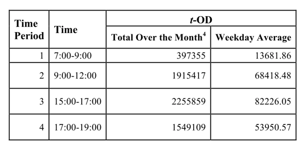
non-186
identical locations) are usually observed with long travel intervals i.e. the first location may be
187
observed at 8:56 and next location may be observed at 18:03 with no information about
188
intermediate locations (if any) or the time when the trip in between these two locations have been
189
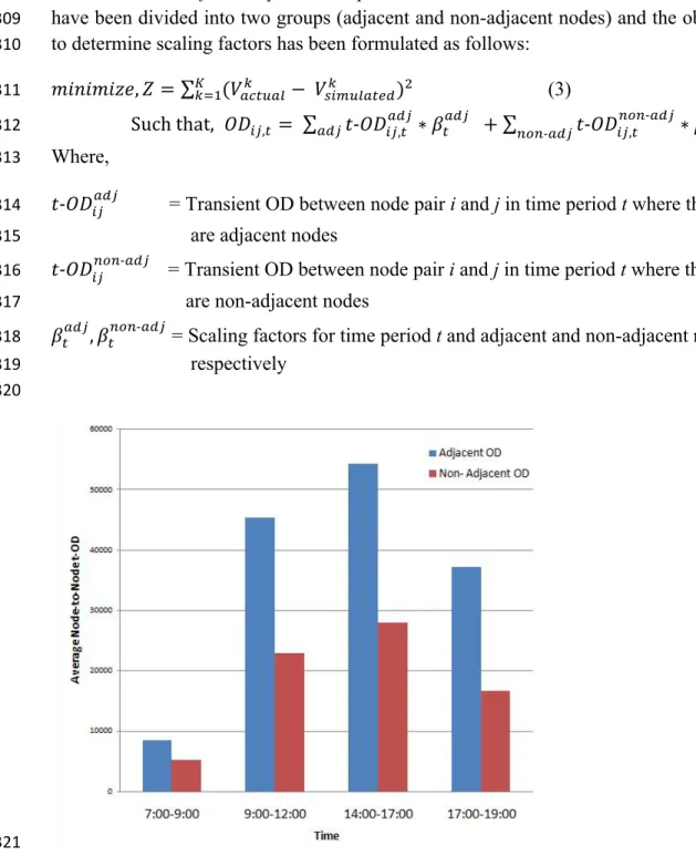
made.
190
Another limitation is the CDR data often records changes in towers in spite of no actual
191
displacement (as the operator balances call traffic among adjacent towers). To better identify
192
timing and origin-destinations of specific trips and reduce the number of false displacements, we
193
therefore extract displacements that have occurred within a specific time window. A lower bound
194
in the time window (10 minutes) is imposed to reduce the number of false displacements without
195
affecting the number of physical displacements occurring within short intervals. An upper bound
196
in the time window (1 hr) is imposed to ensure that meaningful numbers of trips are retained.
197
Therefore, a person trip is recorded if in the CDR, subsequent entries of the same user indicate a
198
displacement (change in tower) with a time difference of more than 10 minutes but less than 1
199
hour.
200
Further, both call volumes (from CDR data) and traffic volumes (from traffic counts) had
201
significant variations throughout the day. Based on correlation analysis of total mobile call
202
volumes and total traffic counts (Figure 6), four time periods (7:00-9:00, 9:00-12:00,
15:00-203
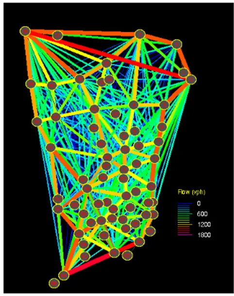
17:00 and 17:00-19:00), have been chosen for analysis.
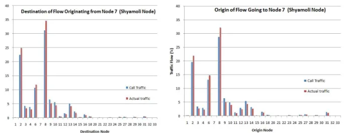
205
206
Figure 6: Hourly variations a. traffic count b. transient ODs from mobile call records
207
3.2 Conversion of tower-to-tower t-OD to node-to-node t-OD
208
For application of the t-ODs in traffic analyses, the origin and destination towers need to be
209
associated with corresponding nodes of the traffic network. The typical tower coverage area can
210
be represented as a combination of three hyperbolas (Figure 7), the size varying depending on
211
tower height, terrain, locations of adjacent towers and number of users active in the proximity
212
(which can vary dynamically).
213
214
Figure 7: Typical coverage area of a tower (http://www.truteq.co.za/tips_gsm/)
The population density in the chosen study area is very high (more than 8111 inhabitants/sq. km
216
(44) and the tower locations are very close to each other (1 km on average). Because of the high
217
user density, it can be assumed that the area between two towers is equally split among the two
218
towers (Figure 8) that is, each tower t has a coverage area (At) approximately defined by a circle
219
of radius 0.5l, where l is the tower-to-tower distance.
220 221
222
Tower 6 and Node 3 need to be added to Figure
223 224
Tower Candidate Node Tower Candidate Node
AAH03JA 20120718 15:54 6 1 AAH03JA 14:54 6 3 1 1 AAH03JA 14:54 3 1 AAH03JA 20120718 16:13 1 2 AAH03JA 16:13 1 1 2 2 Or 1 AAH03JA 16:13 1 1 AAH03JA 20120718 16:15 2 1 AAH03JA 16:15 2 2 Or 1 1 1 AAH03JA 16:15 1 1 AAH03JA 20120718 18:53 1 6 AAH03JA 18:53 1 1 6 3 AAH03JA 18:53 1 3 AAH03JA 20120718 20:49 6 1 AAH03JA 20:49 6 3 1 1 AAH03JA 20:49 3 1 AAH03JA 20120718 23:41 1 6 AAH03JA 23:41 1 1 6 3 AAH03JA 23:41 1 3
ID
ID Call Date Call
Time Origin Tower Destination Tower Origin Node Destination Node Call Time Origin Destination ID Call Time 225
a. Tower-to-tower OD b. Intermediate OD with candidate nodes c. Node-to-node OD
226
Figure 8: Example of tower to node allocation
227
If a unique traffic node i overlaps with At, the calls handled by t are associated with node i (as in
228
the case of Tower 1in Figure 6). However, if At has two (or more) candidate nodes for
229
association, then the candidate nodes are ranked based on the proportion of Atfeeding to each
230
node. That is, the node serving greatest portion of At is ranked 1, the node serving second highest
231
portion of At is ranked 2, etc. For example, in Figure 6, network connectivity (feeder roads) and
232
topography (presence of a canal with no crossing facility in the vicinity) denote that Node 1 and
233
Node 2 are candidate nodes for association with Tower 2. As the major portion of At is connected
234
to Node 2 and the remaining portion is connected to Node 1, they are ranked 1 and 2 respectively
235
for Tower 2. The data format after this step is presented in Figure 7b. As seen in the figure, this
236
typically consists of call records associated with unique nodes and some calls associated with
237
multiple candidate nodes. The calls are then sorted and ranked based on the frequency of the
238
unique nodes used by each user. The frequency of occurrence of the candidate nodes are
compared and used as the basis of replacement. For example, frequency analysis of User
240
“AAH03JA” indicates a higher frequency of Node 1. Therefore, in cases where there are
241
ambiguities between Nodes 2 and 1, Node 1 is used (for this particular user).
242
The same process is used for all users and node-to-node t-OD matrices for each time period of
243
each day are derived.
244 245
3.3 Finding the scaling factor and determining the actual OD matrix
246
As discussed, the node-to-node t-OD matrix (𝑡-‐𝑂𝐷!") provides the trip patterns for developing the
247
actual OD matrix (O𝐷!"). However, in order to determine the actual OD matrix, the t-OD needs to
248
be scaled to match the real traffic flows. A scaling factor 𝛽!" is used in this regard:
249
𝑂𝐷!" = (𝑡 !"
-‐𝑂𝐷!") ∗ 𝛽!"
It may be noted that 𝛽!" takes into account the market penetration rates (i.e. not every user has a
250
mobile phone or uses the specific service provider), the mobile phone non-usage issue (i.e.
251
mobile phone calls are not made from every location traversed by the user), the vehicle usage
252
issue (i.e. users may not use cars for every trip). The potential error introduced due to false
253
displacement (described in Section 2.1) is also accounted for in the scaling factors.
254
The scaling factors are determined using the open-sourced microscopic traffic simulator platform
255
MITSIMLab (42) by applying an optimization based approach. The movements of vehicles in
256
MITSIMLab are dictated by driving behavior models based on decision theories and estimated
257
with detailed trajectory data using econometric approaches. Route choices of drivers are based
258
on a discrete choice based probabilistic model where the utilities of selecting and re-evaluating
259
routes are functions of path attributes, such as path travel times and freeway bias (see 43 for
260
details). The inputs of the simulator include network data, driving behavior parameters and OD
261
matrix. The generated outputs include traffic flow at specified locations in the network.
262
The node-to-node OD matrix derived from the mobile phone data are provided as the initial or
263
seed-OD in this case. The simulated traffic flows are compared with the actual traffic flows
264
extracted from video recordings. The objective function seeks to minimize the difference
265
between the actual and simulated traffic flows in each location by changing the scaling factors.
266
The optimization problem can be represented as follows:
267 268 𝑚𝑖𝑛𝑖𝑚𝑖𝑧𝑒, 𝑍 = (𝑉!"#$!%! − 𝑉 !"#$%&'()! )! ! !!! (1) 269 Such that, 𝑂𝐷!",! = ! 𝑡-‐𝑂𝐷!",!∗ 𝛽!",! !,!!! 270 Where, 271
𝑉!"#$%&'()! = Traffic flow of link k of the road network from simulation
272
𝑂𝐷!",! = Actual OD between nodes i and j in time period t
273
𝑡-‐𝑂𝐷!",! = Transient OD between nodes i and j in time period t
274
𝛽!",! = Scaling factor associated with the node pair i and j and time period t
K = Total number of links for which traffic flow data is available
276
N = Total number of nodes in the network
277 278
However, to make the optimization problem more tractable, group-wise scaling factors are used
279
rather than an individual scaling factor for each OD pair. The grouping is based on the analyses
280
of the CDR data. This simplifies the problem as follows:
281 282 𝑚𝑖𝑛𝑖𝑚𝑖𝑧𝑒, 𝑍 = (𝑉!"#$!%! − 𝑉 !"#$%&'()! )! ! !!! (2) 283 Such that, 𝑂𝐷!",! = !!!!𝑡-‐𝑂𝐷!",!! ∗ 𝛽!! 284 Where, 285
𝑡-‐𝑂𝐷!",!! = Transient OD between node pair i and j in time period t where the node pair i,j
286
belong to group m
287
𝛽!! = Scaling factor for group m and time period t
288
M = Total number of groups of OD-pairs
289 290
4. Results
291
The mobile phone network within the study area comprises of 1360 towers which have been
292
assigned to 29 OD generating nodes (812 OD pairs). Out of the one month CDR data, the
293
weekend data have been discarded. For each day, the calls of each user originating from two
294
different towers in each of the time period have been extracted. After application of the transient
295
trip definitions (displacements occurring more than 10mins but less than 1hr apart) and the tower
296
to node conversion rules (elaborated in Section 3.2), the node-to-node t-ODs are derived. The
297
total number of node-to-node t-ODs are presented in Table 1.
298
Table 1: Node-to-node t-OD
299 300 301 302 303 4 Includes weekends Time Period Time t-OD
Total Over the Month4 Weekday Average
1 7:00-9:00 397355 13681.86
2 9:00-12:00 1915417 68418.48
3 15:00-17:00 2255859 82226.05
Analyses of the node-to-node transient flows indicate that the flows between adjacent nodes are
304
substantially higher than those between non-adjacent nodes (Figure 9). This is reasonable since
305
given the low travel speed in Dhaka, a traveler may not be able to move very far in the 50min
306
time window and the t-ODs mostly capture segments of a longer trip. However, part of it may
307
also be due to the false displacement problem discussed in section 3.1. Therefore, the OD-pairs
308
have been divided into two groups (adjacent and non-adjacent nodes) and the objective function
309
to determine scaling factors has been formulated as follows:
310 𝑚𝑖𝑛𝑖𝑚𝑖𝑧𝑒, 𝑍 = (𝑉!"#$!%! − 𝑉 !"#$%&'()! )! ! !!! (3) 311 Such that, 𝑂𝐷!",! = !"#𝑡-‐𝑂𝐷!",!!"#∗ 𝛽!!"# + !"!-‐!"#𝑡-‐𝑂𝐷!",!!"!-‐!"#∗ 𝛽!!"!-‐!"# 312 Where, 313
𝑡-‐𝑂𝐷!"!"# = Transient OD between node pair i and j in time period t where the node pair i,j
314
are adjacent nodes
315
𝑡-‐𝑂𝐷!"!"!-‐!"# = Transient OD between node pair i and j in time period t where the node pair i,j
316
are non-adjacent nodes
317
𝛽!!"#, 𝛽!!"!-‐!"# = Scaling factors for time period t and adjacent and non-adjacent nodes
318
respectively
319 320
321
Figure 9: Comparison of t-ODs between adjacent and non-adjacent nodes
This yielded eight scaling factors in total that needed to be estimated from the simulation runs of
323
MITSIMLab. Running the optimization process in MATLAB (that invokes MITSIMLab) and
324
using a BOX algorithm (45), the following values of scaling factors have been derived.
325
Table 2: Scaling Factors
326
327
328
It is interesting to note that the scaling factors for adjacent nodes are higher than those of
non-329
adjacent in all time periods other than 15:00-17:00. This does not however indicate that most of
330
the actual trips are to the adjacent nodes (since a full trip may consist of several segments each
331
represented by a separate t-OD).
332
The graphical representation of the t-ODs and actual ODs across the network for one of the time
333
periods and the variations for an example node are presented in Figures 10 and 11 respectively.
334
a. t-OD b. actual OD
335
Figure 10: t-ODs and actual ODs across the network for 7:00-9:00
336
Time Period OD Type Scaling Factor
7:00-9:00 Adjacent 6.787 Non-adjacent 1.712 9:00-12:00 Adjacent 0.971 Non-adjacent 0.345 15:00-17:00 Adjacent 1.647 Non-adjacent 3.407 17:00-19:00 Adjacent 9.404 Non-adjacent 6.779
337
Figure 11: Example of Transient and Actual Traffic Flows To and From a Node (Shyamoli)
338
between 7:00-9:00.
339
5. Validation
340
In addition to the aggregate data used for calibration, traffic counts are collected from four
341
additional locations on a different day. For validation purposes, the scaled up ODs have been
342
applied to simulate the traffic between 9:00-12:00 in MITSIMLab and the simulated traffic
343
counts are compared against the observed counts from these locations. In order to quantify the
344
prediction error, Root Mean Square Error and Root Mean Square Percent Errors have been
345
calculated and are found to be 335.09 and 13.59% respectively.
346
6. Conclusion
347
The main outcome of this research is the methodology for development of the OD matrix using
348
mobile phone CDR and limited traffic count data. The strengths of both data sources are utilized
349
in this approach: the trip patterns are extracted from mobile phones and the ground truth traffic
350
scenario are derived from the counts. The methodology is demonstrated using data collected
351
from Dhaka.
352
There are several limitations of the current research though. Firstly, in this research a simplified
353
objective function with grouped scaling factors has been used. This overlooks the heterogeneity
354
in call rates from different locations (e.g., more calls may be generated to and from railway
355
stations compared to and from offices with land telephone lines, etc.). A more detailed
356
classification of scaling factor can be used to overcome this bias and may yield better results.
357
Moreover, in this particular context, detailed network data and extensive calibration data were
358
not available which may have increased the simulation errors and affected the validation results.
359
However, initial validation results indicate promising success in real life application by transport
360
planners and managers.
Since CDR is already recorded by mobile phone companies for billing purposes, the approach is
362
more economic than the traditional approaches which rely on expensive household surveys
363
and/or extensive traffic counts. It is also convenient for periodic update of the OD matrix and
364
extendable for dynamic OD estimation. This method is particularly effective for generating
365
complex OD matrix where land use pattern is heterogeneous and asymmetry in travelling pattern
366
prevails throughout the day but there is a limitation of traditional data sources.
367
Acknowledgment
368
The data provided for the research has been provided by Grameenphone Ltd. , Bangladesh. The
369
funding for this research was provided by Faculty for the Future Program of Schlumberger
370
Foundation and Higher Education Enhancement Project of the University Grants Commission of
371
Bangladesh and the World Bank.
372 373
References
374 375
1. Hajek, J. J. (1977). Optimal sample size of roadside-interview origin-destination surveys (No. RR
376
208).
377
2. Kuwahara, M., and Sullivan, E. C. (1987). Estimating origin-destination matrices from roadside
378
survey data. Transportation Research Part B,21(3), 233-248.
379
3. Groves, R. M. (2006). Nonresponse rates and nonresponse bias in household surveys. Public 380
Opinion Quarterly, 70(5), 646-675. 381
4. Lo, H. P., Zhang, N., and Lam, W. H. (1996). Estimation of an origin-destination matrix with
382
random link choice proportions: a statistical approach.Transportation Research Part B, 30(4),
383
309-324.
384
5. Van Zuylen, H. J., and Willumsen, L. G. (1980). The most likely trip matrix estimated from
385
traffic counts. Transportation Research Part B,14(3), 281-293.
386
6. Maher, M. (1983). Inferences on trip matrices from observations on link volumes: a Bayesian 387
statistical approach. Transportation Research Part B, 20 (6), 435–447. 388
7. Tebaldi, C., West, M. (1998). Bayesian inference on network traffic using link count data (with 389
discussion). Journal of the American Statistical Association,93, 557–576. 390
8. Li, B. (2005). Bayesian inference for origin–destination matrices of transport networks using the 391
EM algorithm. Technometrics 47 (4), 399–408. 392
9. Cascetta, E. (1984). Estimation of trip matrices from traffic counts and survey data: a generalized 393
least squares estimator. Transportation Research Part B, 18(4–5), 289–299. 394
10. Bell, M. (1991). The estimation of origin–destination matrices by constrained generalized least 395
squares. Transportation Research Part B, 25 (1), 13–22. 396
11. Spiess, H. (1987). A maximum likelihood model for estimating origin-destination matrices, 397
Transportation Research Part B,21(5), 395-412.
398
12. Vardi, Y. (1996). Network tomography: estimating source-destination traffic intensities from link 399
data. Journal of the American Statistical Association,91, 365–377. 400
13. Hazelton, M.L. (2000). Estimation of Origin–Destination matrices from link flows on 401
uncongested networks. Transportation Research Part B, 34 (7), 549–566. 402
14. Hazelton, M.L. (2003). Some comments on origin–destination matrix estimation. Transportation 403
Research Part A, 37 (10), 811–822.
404
15. Hazelton, M.L., 2001b. Inference for origin–destination matrices: estimation, reconstruction and 405
prediction. Transportation Research Part B, 35 (7), 667–676. 406
16. Castillo, E., Menéndez, J., Jiménez, P. (2008). Trip matrix and path flow reconstruction and 407
estimation based on plate scanning and link observations. Transportation Research Part B ,42 408
(5), 455–481. 409
17. Parry, K., & Hazelton, M. L. (2012). Estimation of origin–destination matrices from link counts 410
and sporadic routing data. Transportation Research Part B, 46(1), 175-188. 411
18. Morimura, T., and Kato, S. (2012). Statistical origin-destination generation with multiple sources. 412
21st International Conference on In Pattern Recognition (ICPR), November 11-15, 2012. 413
Tsukuba, Japan. 414
19. Herrera, J., Work D. B., Herring R., Ban X., Jacobson Q., Bayen A. (2010). Evaluation of traffic 415
data obtained via GPS-enabled mobile phones: The Mobile Century field experiment, 416
Transportation Research Part C: Emerging Technologies, 18(4), 568-583.
417
20. http://www.itu.int/en/ITU-D/Statistics/Documents/facts/ICTFactsFigures2013.pdf [accessed
418
20July, 2013] 419
21. Phithakkitnukoon, S., Horanont, T., Di Lorenzo, G., Shibasaki, R., and Ratti, C. (2010). Activity -420
Aware Map: Identifying human daily activity pattern using mobile phone data, Human Behavior 421
Understanding, 6219(3), 14-25,Springer Berlin / Heidelberg.
422
22. Phithakkitnukoon, S., and Ratti, C., (2011), Inferring Asymmetry of Inhabitant Flow using Call 423
Detail Records, Journal of Advances in Information Technology, 2 (4), 239-249. 424
23. Reades, J., Calabrese, F., and Ratti, C. (2009). Eigenplaces: analyzing cities using the space-time 425
structure of the mobile phone network, Environment and Planning B: Planning and Design, 426
36(5), pp. 824-836.
427
24. Wang, P., Hunter, T., Bayen, A. M., Schechtner, K., and González, M. C. (2012). Understanding 428
Road Usage Patterns in Urban Areas. Scientific reports, 2. 429
25. G onzález, M. C., Hidalgo, C. A., and Barabási, A. L.(2008).Understanding individual human 430
mobility patterns, Nature, 453, 779–782. 431
26. Song, C, Koren, T, Wang, P, and Barabási, A. L. (2010). Modelling the scaling properties of 432
human mobility, Nature Physics, 6, 818–823. 433
27. Simini, F., Gonza´lez, M. C., Maritan, A., and Baraba´si, A. L.(2012). A universal model for 434
mobility and migration patterns, Nature, 484, 96–100. 435
28. Candia, J., González, M. C., Wang, P., Schoenharl, T., Madey, G., and Barabási, A. L. (2008). 436
Uncovering individual and collective human dynamics from mobile phone records. Journal of 437
Physics A: Mathematical and Theoretical, 41(22), 224015.
438
29. Sevtsuk, A., and Ratti, C. (2010). Does Urban Mobility Have a Daily Routine? Learning from 439
Aggregate Data of Mobile Networks, Journal of Urban Technology, 17 (1), 41-60. 440
30. Schlaich, J., Otterstätter, T., Friedrich, M., 2010, Generating Trajectories from Mobile Phone 441
Data, TRB 89th Annual Meeting Compendium of Papers, Transportation Research Board of the 442
National Academies, Washington, D.C., USA. 443
31. Becker, R.A., Caceres, R., Hanson, K., Loh, J.M., Urbanek, S., Varshavsky, A., Volinsky, C., 444
Ave, P., Park, F., 2011. Route classification using cellular handoff patterns. In: Proceedings of the 445
13th International Conference on Ubiquitous Computing. ACM, Beijing, China. 446
32. Bolla, R., Davoli, F., and Giordano, A. (2000). Estimating road traffic parameters from mobile
447
communications. In Proceedings 7th World Congress on ITS, Turin, Italy.
448
33. Demissie, M. G., de Almeida Correia, G. H., and Bento, C. (2013). Intelligent road traffic status 449
detection system through cellular networks handover information: An exploratory study. 450
Transportation Research Part C: Emerging Technologies, 32, 76-88. 451
34. Wang J., Wang D. Song X. Sun Di. (2011). Dynamic OD Expansion Method Based on Mobile 452
Phone Location, Fourth International Conference on Intelligent Computation Technology and 453
Automation, Shenzhen, China. 454
35. Caceres, N., Wideberg, J. P., and Benitez, F. G. (2007). Deriving origin destination data from a
455
mobile phone network. Intelligent Transport Systems, IET, 1(1), 15-26.
456
36. Mellegard, E., Moritz, S., and Zahoor, M. (2011, December). Origin/Destination-estimation using
457
cellular network data. In Data Mining Workshops (ICDMW), 2011 IEEE 11th International
458
Conference on (pp. 891-896). IEEE. 459
37. Calabrese F., Lorenzo G. D., Liu L. and Ratti C. (2011). Estimating Origin-Destination Flows 460
using Mobile phone Location Data. IEEE Pervasive Computing, vol. XX, no. XX, 200XX, pp. 461
36–43. 462
38. Wang, P., Hunter, T., Bayen, A. M., Schechtner, K., and González, M. C. (2012). Understanding
463
Road Usage Patterns in Urban Areas. Scientific reports, 2.
464
39. DHUTS. (2010). Dhaka Urban Transport Network Development Study, Draft Final Report. 465
Prepared by Katahira and Engineers International, Oriental Consultants Co. Ltd., and Mitsubishi 466
Research Institute, Inc. 467
40. Grameenphone Ltd. Bangladesh. http://grameenphone.com, accessed on 15.12.2012 468
41. Kritikal Solutions Ltd., India. http://www.kritikalsolutions.com/products/traffic-analyzer.html, 469
accessed on 15.12.2012 470
42. Yang Q. and Koutsopoulos, H. N., (1996). A microscopic traffic simulator for evaluation of 471
dynamic traffic management systems, Transportation Research C, 4(3),113-129 472
43. Ben-Akiva M., Koutsopoulos H. N., Toledo T., Yang Q., Choudhury C. F., Antoniou C., and 473
Balakrishna R. (2010). Traffic simulation with MITSIMLab, in Fundamentals of Traffic 474
Simulation, 1st ed., ser. International Series in Operations Research and Management Science, J. 475
Barceló, Ed. Springer, 233-268. 476
44. Population and Housing Census: Preliminary Results (2011), Bangladesh Bureau of Statistics, 477
Statistics Division, Ministry of Planning, Government of the People’s Republic of Bangladesh 478
45. Box M. J. (1965), A new method of constrained optimization and a comparison with other 479
methods, Computer Journal, 8(1),42-52. 480