Study of the aquatic dissolved organic matter from the Seine River catchment (France) by optical spectroscopy combined to asymmetrical flow field-flow fractionation

(1)

HAL Id: tel-01170629

https://tel.archives-ouvertes.fr/tel-01170629

Submitted on 2 Jul 2015

HAL is a multi-disciplinary open access archive for the deposit and dissemination of sci-entific research documents, whether they are pub-lished or not. The documents may come from teaching and research institutions in France or abroad, or from public or private research centers.

L’archive ouverte pluridisciplinaire HAL, est destinée au dépôt et à la diffusion de documents scientifiques de niveau recherche, publiés ou non, émanant des établissements d’enseignement et de recherche français ou étrangers, des laboratoires publics ou privés.

Study of the aquatic dissolved organic matter from the

Seine River catchment (France) by optical spectroscopy

combined to asymmetrical flow field-flow fractionation

Phuong Thanh Nguyen

To cite this version:

Phuong Thanh Nguyen. Study of the aquatic dissolved organic matter from the Seine River catchment (France) by optical spectroscopy combined to asymmetrical flow field-flow fractionation. Analytical chemistry. Université de Bordeaux, 2014. English. �NNT : 2014BORD0154�. �tel-01170629�

(2)

A THESIS SUBMITTED IN CONFORMITY WITH THE REQUIREMENTS FOR THE DEGREE OF

DOCTOR

UNIVERSITY OF BORDEAUX

DOCTORAL SCHOOL OF CHEMICAL SCIENCES

SPECIALITY: Analytical and Environmental Chemistry

by Phuong Thanh NGUYEN

Study of the aquatic dissolved organic matter from the

Seine River catchment (France) by optical spectroscopy

combined to asymmetrical flow field-flow fractionation

Supervised by: Edith PARLANTI

Defense on Thursday 6 November, 2014

Members of jury:

Ms LESPES Gaëtane, Professor, University of Pau and Pays de l’Adour Reviewer

Mr MOUNIER Stéphane, Lecturer, University of Sud Toulon-Var Reviewer

Mr VARRAULT Gilles, Professor, University of Paris-Est Créteil Examiner

Mr ORANGE Didier, Researcher, IRD - iEES-Paris Examiner

Mr MAZELLIER Patrick, Professor, University of Bordeaux Examiner

(3)

(4)

THÈSE PRÉSENTÉE POUR OBTENIR LE GRADE DE

DOCTEUR DE

L’UNIVERSITÉ DE BORDEAUX

ÉCOLE DOCTORALE SCIENCES CHIMIQUES

SPÉCIALITÉ : Chimie Analytique et Environnementale

Par Phuong Thanh NGUYEN

Étude de la matière organique dissoute aquatique dans le

bassin versant de la Seine (France) par spectroscopie

op-tique combinée au fractionnement par couplage flux/force

avec flux asymétrique

Sous la direction de : Edith PARLANTI

Soutenue le 6 Novembre 2014

Membres du jury :

Mme LESPES Gaëtane, Professeur, Université de Pau et des Pays de l’Adour Rapporteur

M. MOUNIER Stéphane, Maître de Conférences, Université du Sud Toulon-Var Rapporteur

M. VARRAULT Gilles, Professeur, Université Paris-Est Créteil Examinateur

M. ORANGE Didier, Chargé de Recherche, IRD - iEES-Paris Examinateur

M. MAZELLIER Patrick, Professeur, Université de Bordeaux Examinateur

(5)

(6)

Dedicated to

My parents

My husband

My lovely son

(7)

(8)

i

ABSTRACT OF THESIS

Title: Study of the aquatic dissolved organic matter from the Seine River catchment (France)

by optical spectroscopy combined to asymmetrical flow field-flow fractionation.

Abstract: The main goal of this thesis was to investigate the characteristics of dissolved

organic matter (DOM) within the Seine River catchment in the Northern part of France. This PhD thesis was performed within the framework of the PIREN-Seine research program. The application of UV/visible absorbance and EEM fluorescence spectroscopy combined to PARAFAC and PCA analyses allowed us to identify different sources of DOM and highlighted spatial and temporal variations of DOM properties. The Seine River was characterized by the strongest biological activity. DOM from the Oise basin seemed to have more "humic" characteristics, while the Marne basin was characterized by a third specific type of DOM. For samples collected during low-water periods, the distributions of the 7 components determined by PARAFAC treatment varied between the studied sub-basins, highlighting different organic materials in each zone. A homogeneous distribution of the components was obtained for the samples collected in period of flood.

Then, a semi-quantitative asymmetrical flow field-flow fractionation (AF4) methodology was developed to fractionate DOM. The following optimized parameters were determined: a cross-flow rate of 2 ml min-1 during the focus step with a focusing time of 2 min and an exponential gradient of cross-flow from 3.5 to 0.2 ml min-1 during the elution step. The fluorescence properties of various size-based fractions of DOM were evaluated by applying the optimized AF4 methodology to fractionate 13 samples, selected from the three sub-basins. The fluorescence properties of these fractions were analysed, allowing us to discriminate between the terrestrial or autochthonous origin of DOM.

Keywords: dissolved organic matter (DOM); colloids; freshwater aquatic ecosystems;

asymmetrical flow field-flow fractionation (AF4); EEM fluorescence spectroscopy; UV– Visible absorbance; parallel factor analysis (PARAFAC); principal component analysis (PCA); Seine River catchment.

UMR CNRS 5805 EPOC – Oceanic and Continental Environments et Paleoenvironments

LPTC group – Laboratory of environmental and toxicological chemistry

(9)

(10)

iii

RESUME DE LA THESE

Titre : Étude de la matière organique dissoute aquatique dans le bassin versant de la Seine

(France) par spectroscopie optique combinée au fractionnement par couplage flux/force avec flux asymétrique.

Résumé : Le but principal de cette thèse était d'étudier les caractéristiques de la matière

organique dissoute (MOD) dans le bassin versant de la Seine. Ce travail a été réalisé dans le cadre du programme de recherche PIREN-Seine. Les travaux présentés ici visaient plus particulièrement à identifier les sources de MOD et à suivre son évolution dans les zones d’étude. L’analyse des propriétés optiques (UV-Visible, fluorescence) de la MOD, couplée aux traitements PARAFAC et ACP, a permis de discriminer différentes sources de MOD et de mettre en évidence des variations spatio-temporelles de ses propriétés. L’axe Seine, en aval de Paris, a notamment été caractérisé par l'activité biologique la plus forte. La MOD du bassin de l’Oise a montré des caractéristiques plus "humiques", tandis que le bassin de la Marne a été caractérisé par un troisième type spécifique de MOD. Il a d’autre part été mis en évidence la présence de MODs spécifiques dans chaque zone pour les échantillons prélevés en périodes d’étiage, alors qu’une distribution homogène des composants a été obtenue pour l’ensemble des échantillons prélevés en période de crue.

Le rôle environnemental des colloïdes naturels étant étroitement lié à leur taille, il a d’autre part été développé une technique analytique/séparative originale pour l’étude de ce matériel complexe, un fractionnement par couplage flux/force avec flux asymétrique (AF4). Le fractionnement par AF4 des échantillons a confirmé la variabilité spatio-temporelle en composition et en taille de la MOD d'un site de prélèvement à un autre et a permis de distinguer différentes sources de MOD colloïdale confirmant les résultats de l’étude de ses propriété optiques.

Mots Clés : matière organique dissoute (MOD) ; colloïdes ; écosystèmes aquatiques d’eau

douce ; fractionnement par flux/force avec flux asymétrique (AF4) ; spectroscopie de fluorescence EEM ; absorbance UV-Visible ; analyse factorielle parallèle (PARAFAC) ; analyse des composantes principales (ACP) ; Bassin versant de la Seine

UMR CNRS 5805 EPOC - Environnements et Paléoenvironnements Océaniques et Continentaux

Equipe LPTC – Laboratoire de Physico et ToxicoChimie de l’environnement

(11)

iv 1. Contexte des travaux de recherche

La matière organique dissoute (MOD) joue un rôle important pour la biogéochimie des micropolluants influençant potentiellement leur spéciation et leur biodisponibilité. La MOD est un mélange de composés de propriétés chimiques variées et d’origines diverses. Elle est principalement constituée de colloïdes naturels qui sont des macromolécules et nanoparticules ayant une taille variant de 1 nm à 1 μm. De nature très complexe et dynamique, la MOD est un acteur clé dans la dispersion des éléments traces, le transport des contaminants, le cycle du carbone organique et la biodisponibilité des micronutriments et des contaminants.

Le changement climatique exprimé en termes de précipitations, productivité primaire, rayonnement solaire et température entraînera des changements de la qualité et de la concentration en MOD impliquant des modifications du piégeage et de la biodisponibilité des contaminants. Les facteurs contrôlant la qualité et la quantité de la MOD ne sont toujours pas bien compris. Une connaissance plus approfondie de ces processus est nécessaire pour prédire au mieux les changements de la MOD et de ses interactions avec les contaminants. Malgré son importance majeure dans l'environnement sur le devenir des contaminants, les cycles et la composition chimique de la MOD restent mal compris. Il y a, cependant, un réel besoin d’une caractérisation chimique détaillée de la MOD et il est nécessaire d'évaluer l'influence de la variabilité chimique de la MOD sur les processus environnementaux. Le rôle environnemental des colloïdes naturels est d’autre part étroitement lié à leur taille. Néanmoins, le rôle de la taille de la MOD sur ses propriétés d’interaction avec les contaminants est encore méconnu.

Le but principal de cette thèse était d'étudier les caractéristiques de la MOD dans le bassin versant de la Seine. Ce travail a été réalisé dans le cadre du programme de recherche PIREN-Seine (Programme Interdisciplinaire de Recherche sur l'ENvironnement de la Seine - http://www.sisyphe.upmc.fr/piren/) qui est conjointement financé depuis 1989 par le CNRS et les acteurs publics et privés de la gestion de l'eau du bassin de Seine-Normandie. Ce groupement de recherche a pour objectif de développer, à partir de mesures de terrain et de modélisations, une vision d'ensemble du fonctionnement du système formé par le réseau hydrographique de la Seine, son bassin versant et la société humaine qui l'investit. Le bassin de la Seine, 12% du territoire national, supporte le quart de la population de la France, un tiers de sa production agricole et industrielle, et plus de la moitié de son trafic fluvial. Le fonctionnement écologique de l'ensemble du système fluvial et sa modélisation, depuis les bactéries jusqu'aux poissons, sont basés sur l'étude fine des processus physiques, chimiques et biologiques des milieux. Les modèles développés par le PIREN-Seine simulent les variations

(12)

v écologiques et biochimiques de l'hydrosystème, depuis les ruisseaux jusqu'à l'entrée de l'estuaire.

Dans le cadre du bloc « Matière organique » du thème Biogéochimie de l’axe fluvial du programme PIREN-Seine, il était prévu d’étudier spécifiquement la matière organique (MO) dans le bassin versant de la Seine. Le but principal de cette thèse était d'étudier les caractéristiques de la MOD et plus particulièrement d’identifier ses sources et de suivre son évolution dans cet écosystème. Les sources de matière organique dissoute peuvent être multiples :

- Autochtone naturelle : provenant du biote présent dans le milieu (algues, bactéries, macrophytes) ;

- Allochtone naturelle : issue des sols ;

- Allochtone anthropique : rejets urbains domestiques et industriels, rejets liés à l’agriculture. 2. Matériel et méthodes

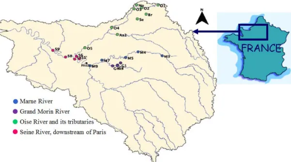
Afin d’identifier ces sources de matière organique, des campagnes « snapshot » ont été menées dans le bassin de la Seine en basses eaux, à deux saisons différentes (automne 2011 et été 2012), et en période de crue (hiver 2013), au cours desquelles 23, 39 et 40 échantillons respectivement ont été prélevés. Ces sites d’échantillonnage étaient répartis sur le bassin de l’Oise, le bassin de la Marne et sur la Seine.

Les deux campagnes de basses eaux ont été menées en novembre 2011 et en août/septembre 2012 à des conditions de débits similaires (environ 100 m3.s-1 à Austerlitz). Le débit restitué par les grands lacs de Seine contribue à environ 50% en août/septembre 2012 contre seulement 20% en novembre 2011 (soutien étiage tardif). La campagne de hautes eaux s’est déroulée en février 2013 avec des débits de 280 m3s-1 pour l’Oise à Creil, de à 700 m3s-1 pour la Seine à Alfortville et de 350 m3s-1 pour la Marne à Gournay.

Les échantillons ont été filtrés immédiatement après le prélèvement sur des filtres en fibre de verre (GF/F 0.7μm; Whatman) préalablement pyrolysés à 450°. Ils ont ensuite été stockés au frais (4°C) et à l’abri de la lumière avant analyses.

La matière organique contenue dans ces échantillons a été caractérisée dans le cadre de cette thèse par les techniques présentées succinctement ci-dessous.

(13)

vi 2.1. La spectroscopie d’absorption UV-visible

Le spectrophotomètre UV-visible utilisé (Jasco V-560) est équipé d’un tube à décharge au deutérium (190 à 350 nm) et d’une lampe à incandescence à filament de tungstène (330 à 900 nm), d’un double monochromateur (réseau plan) pour la sélection des longueurs d’onde et d’un photomultiplicateur (qui permet de transformer l’intensité lumineuse reçue en un signal électrique) comme détecteur. Bien que l’appareil fonctionne en mode double faisceau, il a été utilisé en mode simple faisceau : le signal de référence (cuve + solvant) n’est pas acquis simultanément avec l’échantillon mais avant l’échantillon et soustrait manuellement afin d’utiliser exactement la même cuve dans les deux acquisitions.

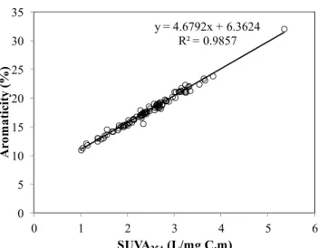
L’une des principales caractéristiques que le spectre d’absorption peut permettre de déterminer est l’aromaticité de la matière organique contenue dans l’échantillon. Deux paramètres sont généralement utilisés pour caractériser l’aromaticité d’un échantillon :

- l’indice SUVA

100 [COD] Abs

SUVA 254

où Abs254 est l’absorbance à 254 nm et [COD] est la concentration en COD en mg/l. - le pourcentage d’aromaticité

Il a été calculé à partir de l’absorbance à 280 nm

6,74 [COD] Abs 0,05 é(%) aromaticit   280 

où Abs280 est l’absorbance à 280 nm et [COD] est la concentration en COD en mol/l.

- le rapport de pentes spectrales SR

Le rapport de pentes spectrales SR (pente 275–295 nm / pente 350–400 nm) calculé à

partir des spectres d’absorbance UV-Visible permet également d’estimer la variation du poids moléculaire de la MOD. Quand SR augmente le poids moléculaire diminue.

2.2. La spectrofluorimétrie

Les spectres de fluorescence ont été enregistrés à l’aide d’un spectrofluorimètre Fluorolog SPEX Jobin-Yvon FL3-22, équipé de doubles monochromateurs à l’excitation et à l’émission. Les échantillons ont été placés dans des cuves en quartz de 1cm de trajet optique, thermostatées à 20°C. Les spectres de fluorescence 3D ont été générés par l’enregistrement successif de 17 spectres d’émission (260-700nm) à des longueurs d’ondes d’excitation prises

(14)

vii tous les 10nm entre 250 et 410 nm. Les spectres 3D des échantillons ont été obtenus par soustraction du spectre 3D d’un blanc d’eau ultrapure (Millipore, Milli-Q).

Les propriétés de fluorescence de la MOD permettent d’obtenir des informations sur la structure et les propriétés générales des macromolécules. La fluorescence est une technique très sensible qui permet de caractériser la MOD à partir d’un échantillon aqueux de faible volume sans nécessité de concentration ou d’extraction. Pour caractériser la MOD, la fluorescence tridimensionnelle (3D ou EEM pour excitation-émission-matrice) est généralement utilisée. Cette technique consiste à accumuler les spectres d’émission acquis pour plusieurs longueurs d’onde d’excitation. Les données quantitatives et qualitatives à prendre en compte sont l’intensité et la position des maxima de fluorescence qui varient en fonction de la nature et de l’origine des échantillons et dépendent des espèces moléculaires fluorescentes qu’ils contiennent.

Le spectre EEM obtenu est interprété par la présence de pics et de rapports d’intensité caractéristiques. Les principales bandes généralement observées pour les eaux naturelles sont mentionnées dans le Tableau ci-dessous.

Les indices de fluorescence HIX et BIX ont également été déterminés afin d’estimer les sources et le degré de maturation de la MOD fluorescente.

La détermination de l’indice d’humification HIX est basée sur le fait que l’avancement des processus d’humification conduit à une augmentation du rapport C/H, i.e. à une augmentation de l’aromaticité de la MOD. Cette augmentation entraîne un déplacement du spectre de fluorescence vers les plus grandes longueurs d’onde d’émission. L’indice HIX est calculé en réalisant le rapport des deux aires définies respectivement par l'intervalle L: 300-345 nm et H: 435-480 nm pour une longueur d'onde d'excitation de 250 nm. L'indice d'humification HIX est alors donné par le rapport H/L.

Pics Longueur d’onde d’excitation (nm)

Longueur d’onde

d’émission (nm) Type de composés

α 330 - 350 420 - 480 Substances type humiques

α’ 250 - 260 380 - 480 Substances humiques + matériel plus récent

β 310 - 320 380 - 420 Matériel récent, composante biologique

γ 270 - 280 300 - 320 Tyrosine, tryptophane ou protéines

(15)

viii Lorsque le degré d’aromaticité de la matière organique augmente, l’indice HIX augmente. En d’autres termes, de fortes valeurs de HIX indiquent la présence d’un matériel organique humifié. Les valeurs de HIX diminuent lorsque la fluorescence de la MOD est déplacée vers les courtes longueurs d’onde, i.e. pour des composés présentant un degré d’aromaticité moins important et des masses moléculaires plus faibles.

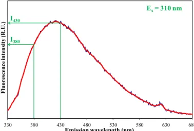
L’indice BIX est calculé à partir du spectre d’émission à 310 nm en divisant l’intensité de fluorescence émise à 380 nm, qui correspond au maximum d’intensité de fluorescence de la bande β quand elle est isolée, par celle émise à 430 nm, qui correspond au maximum de la bande α. Une augmentation de l’indice BIX est liée à une présence plus marquée du fluorophore β dans les échantillons d’eaux naturelles. Puisque le fluorophore β est lié à l’activité biologique autochtone, l’indice BIX permet de juger de la production de matière organique dissoute due à cette activité. Les fortes valeurs de cet indice traduisent une origine autochtone prépondérante de la MOD et la présence de matière organique fraîchement produite dans le milieu.

- PARAFAC

Un algorithme trilinéaire de décomposition nommé PARAFAC (Parallel Factor Analysis) a été utilisé sous le logiciel Matlab (DOMFluor toolbox). PARAFAC est une procédure multidimensionnelle qui permet de traiter un jeu de donnée à 3 dimensions dans sa globalité. C’est une méthode d’analyse de données consistant à construire un modèle linéaire, en estimant les spectres d’excitation et d’émission de F fluorophores et le coefficient appliqué à chacune de ces matrices, afin de pouvoir recomposer le cube de données.

On analyse ainsi un ensemble d’échantillons dans lequel chaque matrice d’excitation et d’émission est un mélange de F composants fluorescents différents.

On considère :

- xi,j,k comme l’intensité de fluorescence d'un échantillon i donné, mesuré au couple de longueurs d’onde d’excitation-émission (j, k),

- ai,f comme facteur de fluorescence (produit de la concentration et du rendement quantique) du fluorophore f (f variant de 1 à F) dans l'échantillon i (variant de 1 à I)

- bi,f comme valeur du spectre d’absorption du fluorophore f à la longueur d’onde j - ci,f comme valeur du spectre d’émission du fluorophore f à la longueur d’onde k - i,j,k comme résidus (bruit et autres variations non expliquées par le modèle)

(16)

ix La loi de Beer–Lambert donne :

i,j,k xi,j,k = Ff=1 ai,f bi,f ci,f + i,j,k

Ainsi à partir d’un jeu d’échantillons comprenant autant de matrices d’excitation et d’émission de fluorescence, les trois inconnues a, b et c sont estimées par PARAFAC en fonction du nombre de fluorophores F fixé et validé pour le modèle le plus approprié, c’est à dire celui présentant des résidus minimum tout en conservant un maximum d’information sans que celle-ci soit répétée. Le modèle a été contraint à la non-négativité des valeurs et le mode « split half analysis » a été utilisé pour valider les composants identifiés.

Il convient d’avoir un nombre élevé d’échantillons pour que l’analyse soit plus précise et le modèle plus fiable.

2.3. Le Fractionnement par couplage Flux/Force avec Flux Asymétrique (AF4)

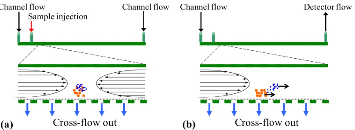
Aujourd’hui, parmi les techniques de séparation en ligne, les systèmes de fractionnement par couplage flux-force (FFF) présentent un grand intérêt pour séparer les différentes fractions colloïdales, car ils possèdent de nombreux avantages par rapport aux techniques chromatographiques, notamment une grande résolution et une large gamme de distribution en taille (de 1 nm à quelques 10 µm). Récemment, de nombreux travaux ont été réalisés grâce au système de fractionnement par couplage flux/force avec flux asymétrique (Asymmetric-Flow Field-Flow Fractionation – AF4), une technique de FFF qui est apparue très prometteuse en terme de pouvoir séparatif et de possibilités de couplage avec des détecteurs variés. Cette technique offre de nouvelles perspectives dans la caractérisation et la séparation des biopolymères, des macromolécules colloïdales et des nanoparticules. C’est une technique qui permet de séparer le matériel colloïdal en fonction de sa taille et représente une alternative aux dispositifs de chromatographie sur colonne. La séparation a lieu dans un canal sans phase stationnaire et permet de déterminer non seulement la taille mais également l’état de dispersion et la forme des colloïdes.

Le système AF4 utilisé est un Eclipse 3 de Wyatt Technology Europe. Il est équipé d’un détecteur UV (HP1200 series, Agilent) et d’un détecteur à diffusion de lumière statique multi-angulaire (3 angles de mesure - miniDAWN TREOS, Wyatt Technology Europe). L’AF4 est équipé d’un canal de séparation court Eclipse avec un espaceur de 490 µm d’épaisseur et d’une membrane Pall Omega en polyethersulfone de seuil de coupure 1 kDa.

(17)

x Les paramètres du fractionnement suivants ont été optimisés dans ce travail : le débit au détecteur, les volumes et temps d’injection, les débits et temps de focus, le type de flux croisé appliqué pendant la phase d’élution. Les conditions opératoires optimales retenues ont été les suivantes :

Le débit au détecteur est maintenu constant à 0,5 ml/min. Après équilibre du débit pen-dant 2 min, 1 ml d’échantillon est injecté à un débit de 0,2 ml/min penpen-dant 6 min avec un flux de focus de 2 ml/min. Le temps de relaxation optimal a été déterminé à 2 min avec un flux de focus de 2 ml/min. Différents programmes de flux croisé pour l’élution ont été testés (cons-tant, gradient linéaire, gradient exponentiel). Les conditions optimales qui ont été retenues pour l’élution sont un flux croisé constant à 3,5 ml/min pendant 15 min, suivi d’un gradient exponentiel de flux croisé de 3,5 ml/min à 0,2 ml/min en 28min.

3. Résultats

3.1. Fluorescence EEM

L’ensemble des échantillons des campagnes « snapshot » de novembre 2011, août/septembre 2012 et février 2013 ont été analysés par fluorescence 3D.

Les concentrations en carbone organique fluorescent en août/septembre 2012 et février 2013 sont plus faibles qu’en novembre 2011. Les échantillons de Seine sont caractérisés par une plus forte proportion de composés de type protéique, notamment pour les échantillons en aval de Paris, traduisant une plus forte activité biologique dans ces eaux.

D’un point de vue qualitatif, l’examen des rapports d’intensités des principales bandes de fluorescence caractéristiques d’un matériel récent et d’origine plutôt autochtone (α’, β et γ) sur la bande α spécifique du matériel le plus humifié, donc plus ancien, est intéressant car il permet d’estimer les contributions relatives des différentes composantes de la MOD et le type de matériel en présence. Les distributions de ces rapports d’intensités des principales bandes de fluorescence en fonction de la teneur en COD ont permis d’observer des variations très nettes de la qualité de la MOD entre les 3 périodes de prélèvement pour les bassins de la Marne et de la Seine alors que les résultats sont moins discriminants pour le bassin de l’Oise.

Les valeurs de ces rapports sont majoritairement plus élevées pour les échantillons de la campagne « snapshot » de 2012. Ceci tend à montrer la présence d’un matériel organique fluorescent plus récent et une plus forte contribution biologique en septembre 2012.

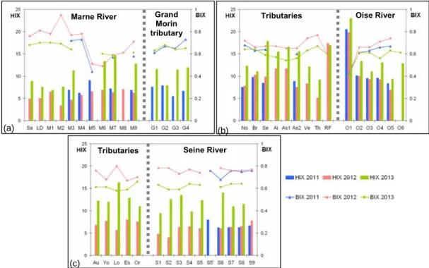
Les indices de fluorescence HIX et BIX ont également montré des variations spatiales de la qualité de la MOD. Les plus fortes valeurs de l’indice HIX, traduisant le matériel organique

(18)

xi le plus mature et aromatique, ont été observées dans le bassin de l’Oise et, de façon logique, les maximales en zones forestières (O1 et RF). L’ensemble des échantillons a globalement été caractérisé par une activité biologique en moyenne relativement élevée (BIX>0.6), les plus fortes valeurs étant observées en Seine en 2011 et 2012 et dans le bassin de la Marne en 2012.

La période de crue (2013) s’est distinguée par de fortes valeurs de HIX alors que les plus faibles valeurs ont été observées en période d’étiage (2012) et majoritairement associées à de fortes valeurs de BIX, traduisant une forte activité biologique pour ces échantillons.

Les matrices d’excitation et d’émission de fluorescence de l’ensemble des 102 échantillons des trois campagnes « snapshot » ont été traitées par PARAFAC. Un modèle à 7 composants a ainsi pu être déterminé, expliquant 99,8 % de la variabilité du jeu de données.

Le composant 4 est similaire au fluorophore β et le composant 6 correspond au matériel de type protéique (fluorophore γ). Les composants 1, 2 et 3, quant à eux, s’apparentent à du matériel de type humique (fluorophores α’ et α).

Les variations de ces 7 composants pour l’ensemble des échantillons ont montré des in-tensités des composants plus fortes en 2011 traduisant des concentrations en matériel fluores-cent plus élevées. Pour 2011 et 2012 nous avons observé des distributions de ces 7 compo-sants très différentes d’un bassin versant à l’autre mettant en évidence des caractéristiques de matériel organique différentes et spécifiques pour chaque bassin. Au contraire, pour la cam-pagne de crue de 2013, la distribution des 7 composants était beaucoup plus homogène avec le composant 1 dominant pour l’ensemble des échantillons et des caractéristiques plus hu-miques traduisant la présence d’un matériel organique majoritaire certainement d’origine ter-rigène.

L’analyse statistique des données a montré une variation temporelle de la distribution des 7 composants représentatifs de la MOD avec un composant 7 bien plus représenté en 2011. Une variation des caractéristiques de la MOD en fonction des sites de prélèvement et une dif-férenciation des sous-bassins étudiés a également été mise en évidence.

Ces variations spatio-temporelles ont notamment montrées des distributions des 7 com-posants dominées par le composant 1 pour l’année 2013 mais également pour le bassin de l’Oise quelque soit la campagne de prélèvement. Le composant 7 semblerait caractériser le sous-bassin de la Marne. Les échantillons de la Seine (2011 et 2012) se sont singularisés avec une signature particulière prédominée par les composants 3, 4 et 5.

(19)

xii 3.2. Absorbance UV – Visible

L’indice SUVA est apparu globalement plus élevé pour les échantillons de la campagne « snapshot » de novembre 2011 sauf pour les échantillons de la Marne et pour S6 où les plus fortes valeurs ont été obtenues en 2013.

L’étude de la variation des rapports des pentes spectrales SR pour l’ensemble des sites et

des campagnes de prélèvement a montré que les échantillons de la Marne (2011 et 2012) étaient caractérisés par le matériel organique de plus faible poids moléculaire. Les échantil-lons de la Seine en 2012 ont également été caractérisés par une MOD de faible poids molécu-laire. Le matériel de plus haut poids moléculaire a été observé pour les échantillons de Grand Morin et les échantillons des trois bassins en 2013. Il n’a pas pu être observé de relations entre poids moléculaire et indice d’humification ou pourcentage d’aromaticité.

3.3. Analyse en composantes principales des données spectroscopiques

Une analyse en composantes principales (ACP) a été réalisée en utilisant comme va-riables les 7 composants déterminés par l’analyse PARAFAC, les indices d’absorbance (SR, %

aromaticité et SUVA), les indices de fluorescence (HIX, BIX, Iα’/Iα, Iβ/Iα et Iγ/Iα) et les in-tensités de fluorescence (Iα’, Iα, Iβ et Iγ) / COD.

Cette ACP a montré que les composants 4, 5, 6 et 7 apparaissent plutôt liés à l’activité biologique. Le composant 4 apparait, comme déjà mentionné, similaire au fluorophore β. Les composants 1, 2 et 3, quant à eux, seraient plutôt liés à l’aromaticité et au matériel de type humique.

L’analyse ACP a permis de différencier les bassins de la Seine, de l’Oise et de la Marne. Les échantillons du sous-bassin de l’Oise sont apparus caractérisés par une MOD plus mature, aromatique alors que ceux des sous-bassins de la Seine et de la Marne présenterait une MOD majoritairement liée à une forte activité biologique.

L’analyse ACP a également permis de différencier les 3 campagnes de prélèvement, fai-sant à nouveau ressortir le caractère plus mature, aromatique de la MOD de l’ensemble des échantillons prélevés en période de crue. Les échantillons de 2011 et 2012 étaient quant à eux caractéristiques d’une forte activité biologique, les échantillons de 2012 se différenciant par de plus faibles poids moléculaires et un caractère plus récent de la MOD.

L’analyse des propriétés optiques de la MOD a donc permis de discriminer différentes sources de matières organiques et de mettre en évidence des variations tant qualitatives que quantitatives de cette MOD. Ces variations sont apparues à la fois liées aux conditions

(20)

hydro-xiii logiques (crue, étiage) et aux spécificités des sites géographiques (différenciation des 3 sous-bassins).

3.4. Fractionnement par couplage Flux/Force avec Flux Asymétrique (AF4) Tous les échantillons des campagnes « snapshot » ont été fractionnés par AF4.

Le bassin de la Marne a été caractérisé par une MOD majoritairement constituée de mo-lécules de petites tailles en bon accord avec les résultats de l’analyse de la variation des rap-ports des pentes spectrales SR. Une seconde population de molécules de taille supérieure est

observée en moindre proportion. Les échantillons du bassin de l’Oise ont montré globalement une population majoritaire de molécules de taille intermédiaire si l’on compare avec celles observées pour le bassin de la Marne. Dans le bassin de la Seine on a observé une distribution avec deux populations en proportions similaires (S6 et S7), les deux de tailles légèrement su-périeures par rapport aux échantillons de la Marne. On a retrouvé cette distribution pour les échantillons G2 et G3 du bassin du Grand Morin. Les distributions observées pour les échan-tillons S5’, S8 et S9 du bassin de la Seine s’apparentent plus aux distributions en taille de mo-lécules des échantillons du bassin de l’Oise de même que pour l’échantillon G1 du bassin du Grand Morin. L’échantillon G4 de ce dernier bassin présentait une distribution en taille simi-laire à celles déterminées pour les échantillons du bassin de la Marne.

On a ainsi observé globalement trois types de distributions en bon accord avec la discri-mination mise en évidence par l’analyse ACP et les résultats de l’analyse de la variation des rapports des pentes spectrales SR. Un premier type est caractérisé par une prédominance de

petites molécules et d’une autre population de taille supérieure (par exemple M7). Le second type serait caractérisé par deux populations en proportions similaires et de tailles légèrement supérieures à celles du type 1 (par exemple S6). La troisième catégorie est constituée d’une seule population de molécules de taille intermédiaire (par exemple Se).

L’étude de la distribution en taille des constituants de la MOD a montré qu’ils étaient globalement de relativement petite taille avec néanmoins une gamme de tailles moléculaires montrant l’hétérogénéité du matériel organique. Les plus hautes valeurs ont été observées pour les échantillons en 2011, et plus particulièrement pour les échantillons de Grand Morin. Ces résultats étaient en bon accord avec ceux relatifs à la variation du rapport de pentes spec-trales SR.

(21)

xiv Des échantillons ont été choisis sur la base de leurs propriétés optiques et de leurs distri-butions en taille observée par AF4 en veillant à leur représentativité des sites des 3 sous-bassins et des différentes périodes d'échantillonnage. Les échantillons qui ont été sélectionnés sont : G1 (2011 et 2013) - Grand Morin ; M7 (2011, 2012 et 2013) - Marne ; O1 (2011, 2012 et 2013) - Oise, zone forestière ; S5 (2012 et 2013) et S6 (2011, 2012 et 2013) - Seine en aval de Paris. Pour ces 13 échantillons 8 à 9 fractions ont été séparées et collectées pour être analy-sées par fluorescence.

Les valeurs les plus basses de BIX ont été systématiquement déterminées pour la 3ème fraction, indépendamment des échantillons considérés, suggérant ainsi la présence dans cette fraction des constituants de MOD d’origine principalement terrestre. Pour tous les échantil-lons considérés, les valeurs les plus fortes de BIX n'ont pas été observées seulement pour les petites tailles moléculaires, montrant que les constituants d'origine autochtone de la MOD peuvent être caractérisés à la fois par des bas ou des hauts poids moléculaires. Des fluoro-phores caractéristiques de pigments ont pu être détectés dans quelques fractions des sous-bassins de l'Oise et de la Marne.

Le fractionnement par AF4 des échantillons a ainsi confirmé la variabilité spatiale et temporelle en composition et en taille de la MOD et a permis de distinguer différents types de matière organique colloïdale.

4. Conclusion et perspectives

L’AF4 a été utilisé pour fractionner dans un continuum de tailles colloïdales les consti-tuants de la MOD d'échantillons d'eau de surface. La combinaison de l’AF4 avec des tech-niques de spectroscopie optique (absorbance UV/Visible et fluorescence) couplée à PARA-FAC et à des analyses statistiques, nous a permis de distinguer différentes sources de matière organique dissoute dans le bassin versant de la Seine et a mis en évidence des variations spa-tiales et temporelles significatives de la MOD ainsi que des typologies de MOD spécifiques des différents sites d'échantillonnage.

La fluorescence EEM couplée à l’AF4 semble ainsi être un outil puissant pour l'étude de la MOD dans l'environnement aquatique et offre de nouvelles perspectives dans la caractérisa-tion et la séparacaractérisa-tion de la MOD colloïdale.

(22)

xv Il serait intéressant de poursuivre l'observation des variations spatio-temporelles des caractéristiques de la MOD dans le bassin versant de la Seine. En effet, bien que la MOD joue un rôle clé dans les processus environnementaux, il y a clairement un manque de connaissances concernant sa caractérisation et un manque de suivi à long terme. Une connaissance plus détaillée des caractéristiques de la MOD est en effet nécessaire si l’on veut d’une part, pouvoir comprendre ses cycles biogéochimiques et les processus mis en jeu dans l’environnement et notamment concernant les interactions MOD/contaminants et, d’autre part, prédire l’impact des changements globaux sur ces processus.

En ce qui concerne le système AF4, il serait intéressant de continuer l'optimisation des paramètres expérimentaux. Il parait particulièrement essentiel en effet de minimiser la perte d'échantillon en testant différents matériaux de membrane ainsi que des seuils de coupure plus petits. De plus, il serait aussi nécessaire d'étudier l'effet de la force ionique de la phase éluante sur l'efficacité de la séparation des macromolécules naturelles.

Il serait de plus important, pour pouvoir étudier les interactions de la MOD avec les contaminants, de coupler la spectrométrie de masse au système de fractionnement par flux/force avec flux asymétrique. D'un point de vue général, compte tenu de la complexité de la matière organique, des écosystèmes environnementaux et des processus d'interactions MOD/contaminants, une approche par détection multidimensionnelle semble essentielle.

(23)

(24)

xvii

ACKNOWLEDGEMENTS

It is my pleasure to write these acknowledgements

I would like to acknowledge the financial support of the Program PIREN-Seine (http://www.piren-seine.fr). All the members involved in the “Organic Matter” part of PIREN Seine project are acknowledged for their help in collecting samples from the Seine River catchment. Especially, I would like to extend my thanks to the members in Laboratory of Water Geochemistry (LGE), Institute of Geophysics (IPGP), Université Paris Diderot, Sorbonne Paris Cité and Laboratory Sisyphe, University Pierre and Marie Curie, Paris, France for providing me with the DOC analysis for all samples collected in the Seine River catchment.

I would like to acknowledge the Vietnamese and French Governments (Embassy of France in Hanoi) for my PhD grant. I am also grateful to the University of Science and Technology of Hanoi for their recruiting of PhD scholars to study in France.

I would like to thank Ms. Gaëtane LESPES and Mr. Stéphane MOUNIER who agreed to be reviewers of my thesis for their insightful comments. I want to thank Mr. Gilles VARRAULT, Mr. Didier ORANGE and Mr. Patrick MAZELLIER for participating in my committee.

I wish to express my deepest gratitude to my supervisor, Dr. Edith PARLANTI, for her guidance, encouragement, and patience during these extended years, especially during the finalizing of this thesis and for not giving up on me. Her expertise in the field of dissolved organic matter improved my research skills and prepared me for future challenges.

I especially want to thank Dr. Hélène BUDZINSKI, the director of the Laboratory of Physical and Toxicological chemistry of the environment, for giving me the opportunity to work in her lab.

(25)

xviii I would like to thank all former and current members of the Laboratory of Physical and Toxicological chemistry of the environment. I truly thank Van Hoi BUI for introducing me about our lab, for all his help throughout my years here in Bordeaux. I am greatly indebted to Marie-Ange CORDIER for her technical advice and her training on lab equipment. Jérémie PAROT, thank you for discussing my data, bringing laughter to me. I am proud to know both you and Marie-Ange. Thanks to Yuzhe GUO for teaching me how to run PARAFAC model in MATLAB. Thanks to Julien GIGAULT for helping with important knowleadge and experience about AF4. I would like to extend my thanks to Maylis SAINT-HUBERT and her mother for all their help. Thanks to Laurène LECUYER, Camille LOPEZ, Stéphanie CUENOT-WOLFF, Jean FROMENT for everyday life in the lab.

I wish to express my sincere thanks to Prof. Céline GUEGUEN (department of chemistry, Trent University, Canada) for giving me the beginning knowledge about AF4.

Thanks to my Vietnamese friends in Bordeaux, anh Minh-Ngoc, anh Dao, chi Hai-Hong, chi Nga, chi Hang, chi Van, chi Trang, chi Huong, anh Tung, ban Dung, ban Tung, em Ha, em Luan, em My Anh, em Truong, em Xuan-Hong, em Lien, em Thanh, em Thao…, who have helped me pass to difficulties in my life when I am here. My special thanks go to my best friend, Minh Thao QUACH, you are the first person to bring a tear to my eye in writing these acknowledgements. You helped me to understand what I was truly meant to do and what truly makes me happiest in life. I cannot stop smiling, I love sharing my life with you. And to my friends in the laBRI, Lorijn, Claire, Nesrine, Omessaad…, thank you for your friendship. I feel lucky to meet all of you in Bordeaux.

Last but not least, the biggest thanks go to my family. Words cannot express my gratitude thanks to my parents, my husband, my brother and my lovely son for all the love and the encouragement they offered me. I dedicate this thesis to them.

(26)

xix

LIST OF ACRONYMS

a : absorption coefficient (m-1)

AsFFFF or AF4 : Asymmetric flow field-flow fractionation BIX : biological autochthonous input index

CDOM : coloured or chromophoric dissolved organic matter CF : cross-flow rate during elution time (ml/min)

DBPs : disinfection byproducts

DF : Detector or channel flow (ml/min)

DLS : dynamic light scattering

DOC : Dissolved Organic Carbon

DOM : dissolved organic matter

EEM : excitation-emission matrix

EEMs : excitation-emission matrix spectral

ETM : estuarine turbidity maximum

FDOM : fluorescent dissolved organic matter

FF : cross-flow rate during focusing time (ml/min) FFF : field flow fractionation

FIFO frit inlet/frit outlet–flow field-flow fractionation FlFFF : flow field flow fractionation

FTIR : Fourier Transform InfraRed

HAAs : haloacetic acids

HIX : humification index

HMW : high molecular weight

HPIA : Hydrophilic acid fraction HPIA : Hydrophilic acid fraction HPIN : Hydrophilic neutral fraction

HPLC : high performance liquid chromatography HPOA : Hydrophobic acid fraction

HPOB : Hydrophobic base fraction

HPON : Hydrophobic neutral fraction

HPSEC : High pressure size exclusion chromatography

HSs : humic substances

ICP-MS : inductively coupled plasma mass spectroscopy IHSS : International Humic Substances Society

LMW : low molecular weight

MALLS : laser light scattering

Mn : number-average

MP : mobile phase composition

MS : mass spectrometry

Mw : weight-average

(31)

xxiv MWCO : molecular weight cut off

NDIR : non dispersive infrared detector

NMR : Nuclear Magnetic Resonance

NOM : natural organic matter

NPOC non-purgeable organic carbon

PAHs : polycyclic aromatic hydrocarbons PARAFAC : parallel factor analysis

PCA : Principal component analysis

PDI : polydispersity index

PES : polyethersulfone

PSS : polystyrenesulfonate

R : retention ratio

RC : regenerated cellulose

rgw : weight-average radius of gyration

RI : differential refractive index

RMM : relative molar mass

S : spectral slope

SEC : size exclusion chromatography

SR : spectral slope ratio

SRFA : Suwannee River fulvic acid

SRHA : Suwannee River humic acid

SUVA : specific ultraviolet absorption tf : relaxation or focus time (min)

THMs : trihalomethanes

to : void time (min)

TOC : total dissolved organic carbon

tR : retention time (min)

UV : Ultraviolet

UV-Vis : Ultraviolet visible

(32)

xxv

LIST OF TABLES

Table 1.1 Compositions of NOM fractions and chemical groups Table 1.2 Main fluorescence bands for natural waters

Table 1.3 Summary of FlFFF operational conditions and main conclusions of DOM studies

Table 2.1 List of sampling sites and their codes

Table 2.2 DOM characteristics associated with the range of values obtained for the HIX and BIX indices from estuarine and seawater samples

Table 3.1 UV–Visible absorbance parameters of surface water samples in the Seine River catchment

Table 3.2 Spearman coefficients of correlation (P<0.01, n=102) between ratios of fluorescent intensities to DOC concentration

Table 3.3 Spatial Mann-Whitney U-test analysis for comparison of HIX values during the three sampling events

Table 3.4 Spatial Mann-Whitney U-test analysis for comparison of BIX values during the three sampling events

Table 3.5 Characteristics of the seven component model determined by PARAFAC in this work compared to previous studies

Table 3.6 Regression analysis of logarithmic correlation between EEM-PARAFAC components

Table 3.7 Correlation coefficients between ratios of intensities of EEM-PARAFAC components with fluorescence indices

Table 5.1 Number-average (Mn), weight-average (Mw), peak (Mp) molecular weights

and polydispersity index (PDI) of lower-molecular weight fraction determined at 280 nm using UV detection

Table 5.2 EEM contour plots (intensity scales different) of the bulk samples and the nine AF4 fractions isolated for O1 (2011, 2012 and 2013) in the Oise River

Table 5.3 EEM contour plots (intensity scales different) of the bulk samples and the eight AF4 fractions isolated for G1 (2011 and 2013) in the Grand Morin tributary

Table 5.4 EEM contour plots (intensity scales different) of the bulk samples and the nine AF4 fractions isolated for M7 (2011, 2012 and 2013) in the Marne River

(33)

xxvi Table 5.5 EEM contour plots (intensity scales different) of the bulk samples and the nine

AF4 fractions isolated for S5 (2012 and 2013) in the Seine River

Table 5.6 EEM contour plots (intensity scales different) of the bulk samples and the nine AF4 fractions isolated for S6 (2011, 2012 and 2013) in the Seine River

(34)

xxvii

LIST OF FIGURES

Figure 1.1 The continual size of natural organic matter in the aquatic environment Figure 1.2 Two proposed models of molecular structure of humic substances

Figure 1.3 Normalized emission spectra (at excitation wavelength 310 nm) of samples in the Gironde Estuary in a range of variable salinity (S = 0 to 34.3)

Figure 1.4 Basic separation principle of flow field flow fractionation

Figure 2.1 Location of sampling sites in 2011 in the Seine River catchment, France Figure 2.2 Location of sampling sites in 2012 (low-water) in the Seine River catchment,

France

Figure 2.3 Location of sampling sites in 2013 (flood) in the Seine River catchment, France

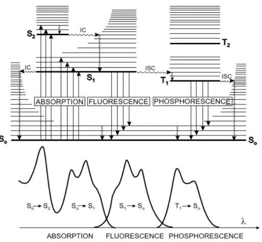
Figure 2.4 Perrin–Jablonski diagram and illustration of the relative positions of absorption, fluorescence and phosphorescence spectra

Figure 2.5 UV-visible absorption spectrum (sample Mery/ Seine-S1, 2012)

Figure 2.6 Emission spectrum at the excitation wavelength 370 nm to calculate the f450/f500 index (sample Mery/ Seine-S1, 2012)

Figure 2.7 Emission spectrum at the excitation wavelength 254 nm to calculate the HIX index

Figure 2.8 Emission spectrum at the excitation wavelength 310 nm to calculate the BIX index

Figure 2.9 Two main types of FlFFF

Figure 2.10 Principle of the separation of macromolecules by FlFFF Figure 2.11 Field flow fractionation fractogram

Figure 3.1 DOC concentrations for samples collected in November 2011 Figure 3.2 DOC concentrations for samples collected in 2012

Figure 3.3 DOC concentrations for samples collected in 2013

Figure 3.4 Variations of relationship between SUVA254 and Aromaticity in the Seine

River catchment

Figure 3.5 Variations of specific ultraviolet absorbance (SUVA254) (L.m-1.mg-1C) in the

three studied basins

Figure 3.6 Variation of the spectral slope ratio SR in theSeine River catchment during

the three sampling periods

Figure 3.7 Variations of (a) spectral slope ratio SR and (b) SUVA254 as a function of

DOC concentration

Figure 3.8 Variations of fluorescence intensities of (a) α’; (b) α; (c) β and (d) γ bands as a function of DOC concentrations in the Seine River catchment during the three campaign periods

Figure 3.9 Box plots of fluorescence intensities normalized to DOC concentration Figure 3.10 Distribution of Iα’/Iα ratio as a function of DOC concentration in the Marne

(a), Oise (b) and Seine (c) basins during the three snapshot campaigns Figure 3.11 Distribution of Iβ/Iα ratio as a function of DOC concentration in the Marne

(35)

xxviii Figure 3.12 Distribution of Iγ/Iα ratios as a function of DOC concentration in the Marne

(a), Oise (b) and Seine (c) basins during the three snapshot campaigns Figure 3.13 Variations of the f450/f500 index as a function of DOC concentration

Figure 3.14 Variations of HIX and BIX for samples in the Marne (a), Oise (b) and Seine (c) basins during the three snapshot campaigns

Figure 3.15 Variations of HIX (a) and BIX (b) indices as a function of DOC concentration

Figure 3.16 Variations of BIX index (a) and spectral slope ratio SR (b) as a function of

HIX index

Figure 3.17 (a) Contour plots of the seven components identified by PARAFAC analysis, and (b) Excitation (solid lines) and Emission loadings (dotted lines) of each component

Figure 3.18 Examples of measured (a-d), modeled (e-h) and residual (i-l) EEMs for different DOM in the catchment. Fluorescence emission is in Raman units Figure 3.19 Distribution of the fluorescence intensity normalized to DOC of the 7

Figure 3.20 Relative percentage distributions of the 7 components identified by PARAFAC in the three studied basins in (a) 2011; (b) 2012 and (c) 2013 Figure 3.21 Distribution of the 7 components identified by PARAFAC by river basin

and among periods of sampling.

Figure 3.22 Ratios of the average fluorescence maximum of each component to the fluorescence maximum of C2 during the three sampling times

Figure 3.23 Variations of relationships between fluorescence maximum of pairs of components in the Seine River catchment

Figure 3.24 Variations of relationships between fluorescence maximum of pairs of components in the Seine River catchment

Figure 3.25 Principal component score plot of the total variance from data set

Figure 4.1 Location of six sampling sites in 2012 in the Seine River catchment, France Figure 4.2 Correlation between cross-flow rate (Vc) and the retention time (tR) of small

fractions of DOM macromolecules of sample Beaumont (O5) collected in 2012

Figure 4.3 Cross-flow rate during different phases of a programmed cross-flow separation

Figure 4.4 Effect of different cross-flow program form on the separation of DOM macromolecules of sample Mery (S1) collected in 2012

Figure 4.5 Fractograms of small fractions of DOM obtained by UV detector as a function of focus time.

Figure 4.6 EEM spectra of (a) bulk sample Mery (S1- 2012), (b) fraction collected for tf

=0 min, (c) fraction collected for tf =2 min

Figure 4.7 Fractograms for 6 samples from the Seine River catchment in the optimized conditions obtained by (a) UV and (b) MALLS detectors

Figure 5.1 (a) UV fractogram of standards, and (b) UV calibration curve obtained between molecular weight and retention time of standards

(36)

xxix 2013

Figure 5.3 UV fractograms of samples collected in (a) Marne River and (b) Grand Morin tributary in 2011

Figure 5.4 UV fractograms of samples collected in (a) Oise River and (b) its tributaries in 2011

Figure 5.5 UV fractograms of samples collected in Seine River in 2011 Figure 5.6 Variations of Mp in the four basins

Figure 5.7 Comparison of Mp and SR for all the samples collected in 2011

Figure 5.8 Distributions of (a) DOC, (b) PDI, (c) HIX, (d) SUVA, (e) Mp, (f) SR, (g) BIX and (h) Iγ/Iα for the 13 samples selected for fractionation

Figure 5.9 AF4 fractograms of the samples M7 collected both in 2011, 2012 and 2013 Figure 5.10 AF4 fractograms of the samples G1 collected both in 2011 and 2013 Figure 5.11 AF4 fractograms of the samples O1 collected both in 2011, 2012 and 2013 Figure 5.12 AF4 fractograms of samples S5 (a) and S6 (b) fractionated for the Seine

River

Figure 5.13 Examples of EEM spectra of DOM in the Seine River catchment

Figure 5.14 Positions of all fluorescence intensity maxima identified within EEM spectra for all fractions of samples O1 collected in the Oise River (a) in 2011 (b) in 2012 and (c) in 2013

Figure 5.15 Emission spectra of nine fractions from sample O1 collected in 2011 at Ex =

310 nm

Figure 5.16 Variations of the fluorescence intensity of the bands ’,  and  between the nine fractions and the three sampling dates for O1 in the Oise River Figure 5.17 Variations of BIX between fractions compared to bulk samples for site O1

in 2011, 2012 and 2013

Figure 5.18 Positions of all fluorescence intensity maxima identified within EEM spectra for all fractions of samples G1 collected in the Grand Morin River (a) in 2011 and (b) in 2013

Figure 5.19 Variations of the fluorescence intensity of the bands ’,  and  between the eight fractions and the sampling dates 2011 and 2013 for sample G1 Figure 5.20 Positions of all fluorescence intensity maxima identified within EEM

spectra for all fractions of samples M7 collected in the Marne River (a) in 2011, (b) in 2012 and (c) in 2013

Figure 5.21 Variations of the fluorescence intensity of the bands ’,  and  between the nine fractions and the three sampling dates for M7 in the Marne River Figure 5.22 Variations of BIX between fractions compared to bulk samples for site M7

in 2011, 2012 and 2013

Figure 5.23 Positions of all fluorescence intensity maxima identified within EEM spectra for all fractions of samples S5 collected in the Seine River (a) in 2012 and (b) in 2013

Figure 5.24 Variations of the fluorescence intensity of the bands ’,  and  between the nine fractions isolated by AF4 for samples S5 collected in 2012 and in 2013 in the Seine River

Figure 5.25 Positions of all fluorescence intensity maxima within EEM, identified in all fractions of sample S6 collected in the Seine River (a) in 2012, (b) in 2012

(37)

xxx and (c) in 2013

Figure 5.26 Variations of the fluorescence intensity of the bands ’,  and  between the nine fractions and the three sampling dates for S6 collected in the Seine River

Figure 5.27 Variations of BIX between fractions compared to bulk samples for the sites (a) S5 (2011 and 2012) and (b) S6 (2011, 2012 and 2013) in the Seine River

(38)

1

(39)

General introduction

(40)

3 The PIREN-Seine research program (Programme Interdisciplinaire de Recherche sur l’ENvironnement de la Seine), a large interdisciplinary research program on the Seine River System jointly financed since 1989 by the French CNRS (National Center for Scientific Research) and the public and private actors of the management of the water of the Seine-Normandy basin, accompanied and contributed to the recent progress in the aquatic science. The aim of the program was to understand the biogeochemical and ecological functioning of the Seine River system at the level of its whole drainage network (from headwaters to the coastal zone), in relation to land use and the environmental management in the watershed (Billen et al., 2007).

For its 6th phase, the PIREN-Seine program suggested structuring its works around 5 main areas of research:

 What agriculture for tomorrow?

 Interfaces between ground water and river  Biogeochemistry of the River

 The determinants of the ecological quality of the aquatic ecosystem  Contaminations during long term period

They were drawn to answer the majority of the questionings of the partners, in coherence with the current stakes identified for the Seine basin by its main actors.

The study of the organic matter is a part of the 3rd section “Biogeochemistry of the River”, which main objective is to study the characteristics of dissolved organic matter (DOM) with the aim of identifying its sources and tracing its evolution and behavior in the Seine River catchment.

DOM in aquatic environments represents one of the largest reservoirs of carbon. It plays an important environmental role not only in the biogeochemical cycles of carbon but also in the transport, stability, speciation, bioavailability and toxicity of pollutants. Generally, DOM originated from three major sources (Mostofa et al., 2013):

(41)

4 2. Autochthonous origins from the degradation of algae or phytoplankton

3. Anthropogenic origins mainly from agricultural, industrial and sewage effluents as well as human activities

Moreover, colloids constitute the bulk of the dissolved organic matter (DOM) in aquatic environments and also play a crucial role in many physical, chemical and biological processes in the ecosystem (Dubascoux et al., 2008). To better understand the composition of environmental colloids as well as their interactions with pollutants, it is necessary to separate these substances according to their properties, especially in terms of their size.

This PhD thesis aims to develop an analytical technique (asymmetrical flow field-flow fractionation) in order to partition DOM into different size fractions whose fluorescence properties will be evaluated.

The results of these works reported in this manuscript thesis which is divided into five chapters.

 The first chapter provides a literature review on dissolved organic matter and the common analytical techniques utilized to fractionate DOM are also reviewed.

 The second chapter describes the study sites within the Seine River catchment and the various analytical techniques as well as the statistical tools which were implementedto characterize and fractionate DOM. Forty-five sites were thus sampled along three sub-basins within the Seine River catchment including the Marne River and its tributary (Grand Morin River) the Oise River and the Seine River.

 The third chapter presents the optical properties of the surface water samples collected during three sampling campaigns.

 The fourth chapter deals with the optimization of a methodology suitable for DOM fractionation.

 Finally, the fifth chapter presents the molecular weight distribution of DOM for the various samples collected from the Seine river catchment and the investigation of fluorescence properties of the isolated DOM fractions for selected samples.

(42)

Chapter I: Bibliographic synthesis

5

(43)

(44)

7 1.1. Overview about natural organic matter

Natural organic matter (NOM) is a highly complex mixture of organic compounds composed of the decay of living organisms in aquatic and terrestrial environments. NOM is ubiquitous in water (Chen M.et al., 2010; Chin et al., 1998; Lam et al., 2007; Penru et al., 2013; Repeta et al., 2002; Rosario-Ortiz et al., 2007; Shon et al., 2006; Thomas, 1997), soil (Akagi et al., 2007; Fellman et al., 2008b; Semenov et al., 2013) and sediments (Burdige, 2005, 2001; Mayer et al., 2006; Wang and Mulligan, 2006). NOM in aquatic ecosystem can be divided into two categories: dissolved and particulate phases. There is no natural cut-off existing between these two fractions and this is still an operational distinction. These two fractions are traditionally separated on the rather arbitrary criteria of filter pore sizes typically in the range of 0.1 to 0.8μm (Asmala et al., 2013). The continuum size of organic matter in aquatic environments is shown in Figure 1.1.

Figure 1.1 The continual size of natural organic matter in the aquatic environment (Aiken et al., 2011)

Of the two categories, dissolved phase, named dissolved organic matter (DOM), plays an essential role in shaping aquatic ecosystems because of the number of processes in which it becomes involved.

(45)

8 Firstly, DOM has been recognized as an important reservoir of oceanic organic carbon with a pool size of roughly 685 ×1015 C (Hansell, 2001). The total transport of organic carbon to the ocean is estimated in the range of 0.4 to 0.9 x 1015_{g year}-1_{(Griffith et al., 2012; Jahnke, 1996;}

Schlesinger and Melack, 1981). Changes in the production or consumption of DOM could lead to significant perturbations of the global carbon cycle.

Secondly, DOM could interact with a large number of organic and inorganic pollutants in aquatic environment such as metals, pesticides, polycyclic aromatic hydrocarbons (PAHs) (Backhus et al., 2003; Guéguen et al., 2004; Koukal et al., 2003) and therefore influence their speciation, solubility, toxicity, transport and bioavailability.

In addition, DOM is also involved in aqueous photochemical reactions, nutrients cycling and availability (Bormann and Likens, 1967). It plays a role as the major light absorbing material in aquatic ecosystems where it absorbs biologically harmful UV light and protects corals and other light-sensitive organism from UV radiation (Anderson et al., 2001; Cory et al., 2004). Furthermore, DOM exerts a strong control in the formation of disinfection byproducts (DBPs), for example, trihalomethanes (THMs) and haloacetic acids (HAAs), during the drinking water supply treatments with disinfectants (Kraus et al., 2008; Pifer and Fairey, 2012).

Taking into account all the factors above, it is essential for us to study about DOM in order to better understand the nature and properties of dissolved organic matter in the aquatic ecosystem.

1.2. Source of DOM in aquatic environment

DOM present in the aquatic system originates from three major sources: autochthonous, allochthonous and anthropogenic sources (McKnight and Aiken, 1998; Mostofa et al., 2009). The autochthonous inputs are derived from the degradation and excretion of algal biomass, submerged aquatic vegetation, seagrass, bacteria, macrophytes and phytoplankton (Boyd and Osburn, 2004; Henderson et al., 2008; McKnight et al., 1998; Wada et al., 2007; Wang et al., 2007; Wu and Tanoue, 2002; Yamashita and Tanoue, 2004; Zhang Yunlin et al., 2009). Photoinduced respiration and microbial respiration or assimilation of algae or phytoplankton and bacteria are two key processes to produce and release new DOM into natural water (Mostofa et al., 2013a). It has been estimated that more than 97% of autochthonous DOM in

(46)

9 fresh water lakes and wetlands originated from macrophytes, while phytoplankton is the basic source of DOM in large lakes and oceanic systems (Søndergaard et al., 2004). There are a number of factors influencing the release process of DOM in water by algae, phytoplankton and bacteria such as: occurrence of the phytoplankton species or microbes, water quality, water temperature, the presence of nutrients, metabolic abilities or inabilities and so on (Gobler et al., 2004; Keller and Hood, 2011; Pete et al., 2010; Puddu et al., 2003; Rochelle-Newall et al., 2011).

On the other hand, the main allochthonous inputs are derived from terrestrial soil organic matter and the degradation of plant in the surrounding watershed (McKnight et al., 2001). DOM from terrestrial ecosystem has a high content of humic material and very complex chemistry (Søndergaard et al., 2004). Terrestrial humic substances (fulvic and humic acids) are known as the dominant DOM fractions in river environments (Malcolm, 1985).

Allochthonous DOM originating from plant materials or particulate detrital pool is significantly different in various regions (tropical, temperate and boreal) due to some factors such as: physical and chemical parameters as well as microbial processes (Mostofa et al., 2013a). The origin of allochthonous DOM from microbial processes can be estimated from significant fluctuation in respired organic carbon in different soil environments. Furthermore, a small proportion of allochthonous aquatic DOM originates from wind-blown material, direct precipitation and leaf fall. Allochthonous DOM differs from autochthonous DOM in several optical (McKnight et al., 1994) and chemical characteristics (Benner, 2002).

The anthropogenic source of DOM typically comes from agricultural, industrial and sewerage effluents as well as human activities (Mostofa et al., 2010). These anthropogenic and human activities released a large number of organic contaminants such as fluorescence whitening agents, phenols, pesticides, PAHs, pharmaceuticals and so on in natural waters (Huang et al., 2010; Kramer et al., 1996; Meng et al., 2013; Morvan et al., 2006; Mostofa et al., 2013; Parinos et al., 2013; Rawn et al., 2001; Yamaji et al., 2010). These organic pollutants could be assimilated by littoral benthos and this is an important pathway for transfer of anthropogenic-associated contaminants to fish or directly to microorganisms (Fu et al., 2010).