Lower tropospheric ozone over the North China Plain: variability and trends revealed by IASI satellite observations for 2008–2016

HAL Id: hal-02364072

https://hal.archives-ouvertes.fr/hal-02364072

Submitted on 30 Oct 2020

HAL is a multi-disciplinary open access

archive for the deposit and dissemination of

sci-entific research documents, whether they are

pub-lished or not. The documents may come from

teaching and research institutions in France or

abroad, or from public or private research centers.

L’archive ouverte pluridisciplinaire HAL, est

destinée au dépôt et à la diffusion de documents

scientifiques de niveau recherche, publiés ou non,

émanant des établissements d’enseignement et de

recherche français ou étrangers, des laboratoires

publics ou privés.

Lower tropospheric ozone over the North China Plain:

variability and trends revealed by IASI satellite

observations for 2008–2016

Gaelle Dufour, Maxim Eremenko, Matthias Beekmann, Juan Cuesta, Gilles

Foret, Audrey Fortems-Cheiney, Mathieu Lachatre, Weili Lin, Yi Liu, Xiaobin

Xu, et al.

To cite this version:

Gaelle Dufour, Maxim Eremenko, Matthias Beekmann, Juan Cuesta, Gilles Foret, et al.. Lower

tropospheric ozone over the North China Plain: variability and trends revealed by IASI satellite

observations for 2008–2016. Atmospheric Chemistry and Physics, European Geosciences Union, 2018,

18 (22), pp.16439-16459. �10.5194/acp-18-16439-2018�. �hal-02364072�

https://doi.org/10.5194/acp-18-16439-2018 © Author(s) 2018. This work is distributed under the Creative Commons Attribution 4.0 License.

Lower tropospheric ozone over the North China Plain: variability

and trends revealed by IASI satellite observations for 2008–2016

Gaëlle Dufour1, Maxim Eremenko1, Matthias Beekmann1, Juan Cuesta1, Gilles Foret1, Audrey Fortems-Cheiney1, Mathieu Lachâtre1, Weili Lin2, Yi Liu3, Xiaobin Xu4, and Yuli Zhang3

1_{Laboratoire Inter-Universitaire des Systèmes Atmosphériques (LISA), UMR7583,}

Universités Paris-Est Créteil et Paris Diderot, CNRS, Créteil, France

2_{College of Life and Envirenmental Sciences, Minzu University of China, Beijing, China} 3_{Institute of Atmospheric Physics, Chinese Academy of Sciences, Beijing, China}

4_{Key Laboratory for Atmospheric Chemistry of China Meteorological Administration,}

Chinese Academy of Meteorological Sciences, Beijing, China Correspondence: Gaëlle Dufour (gaelle.dufour@lisa.u-pec.fr) Received: 25 April 2018 – Discussion started: 7 June 2018

Revised: 6 November 2018 – Accepted: 7 November 2018 – Published: 20 November 2018

Abstract. China is a highly polluted region, particularly the North China Plain (NCP). However, emission reductions have been occurring in China for about the last 10 years; these reduction measures have been in effect since 2006 for SO2 emissions and since 2010 for NOx emissions. Recent

studies have shown a decrease in the NO2tropospheric

col-umn since 2013 that has been attributed to the reduction in NOx emissions. Quantifying how these emission reductions

translate regarding ozone concentrations remains unclear due to apparent inconsistencies between surface and satellite ob-servations. In this study, we use the lower tropospheric (LT) columns (surface – 6 km a.s.l. – above sea level) derived from the IASI-A satellite instrument to describe the variability and trend in LT ozone over the NCP for the 2008–2016 pe-riod. First, we investigate the IASI retrieval stability and ro-bustness based on the influence of atmospheric conditions (thermal conditions and aerosol loading) and retrieval sen-sitivity changes. We compare IASI-A observations with the independent IASI-B instrument aboard the Metop-B satel-lite as well as comparing them with surface and ozonesonde measurements. The conclusion from this evaluation is that the LT ozone columns retrieved from IASI-A are reliable for deriving a trend representative of the lower/free tropo-sphere (3–5 km). Deseasonalized monthly time series of LT ozone show two distinct periods: the first period (2008–2012) with no significant trend (< − 0.1 % yr−1) and a second pe-riod (2013–2016) with a highly significant negative trend of

−1.2 % yr−1, which leads to an overall significant trend of −0.77 % yr−1for the 2008–2016 period. We explore the dy-namical and chemical factors that could explain these nega-tive trends using a multivariate linear regression model and chemistry transport model simulations to evaluate the sensi-tivity of ozone to the reduction in NOx emissions. The

re-sults show that the negative trend observed from IASI for the 2013–2016 period is almost equally attributed to large-scale dynamical processes and emissions reduction, with the large El Niño event in 2015–2016 and the reduction of NOx

emissions being the main contributors. For the entire 2008– 2016 period, large-scale dynamical processes explain more than half of the observed trend, with a possible reduction of the stratosphere–troposphere exchanges being the main con-tributor. Large-scale transport and advection, evaluated using CO as a proxy, only contributes to a small part of the trends (∼ 10 %). However, a residual significant negative trend re-mains; this shows the limitation of linear regression mod-els regarding their ability to account for nonlinear processes such as ozone chemistry and stresses the need for a detailed evaluation of changes in chemical regimes with the altitude.

16440 G. Dufour et al.: Lower tropospheric ozone over the North China Plain: variability and trends 1 Introduction

Rapid economic development and urbanization in China over the last 3 decades has resulted in increasing pollutant emis-sions; this has led to the highest pollutant concentrations in the world, which largely exceed the recommended outdoor air pollutant thresholds from the World Health Organization (WHO). Several studies have pointed toward a general ozone (O3) increase over some parts of China at the surface (e.g.,

Cooper et al., 2014; Lu et al., 2018; Ma et al., 2016; Wang et al., 2009), in the lower troposphere (e.g., Ding et al., 2008; Sun et al., 2016; Wang et al., 2017b), or in the entire tropo-sphere (e.g., Chen et al., 2015; Verstraeten et al., 2015; Wang et al., 2012; Xu and Lin, 2011). This increase is mainly at-tributed to the emission increase. Only a few long-term O3

measurements are available in China. Wang et al. (2009) re-ported an increase of surface O3of 0.58 ppb yr−1during the

1994–2007 period at a regional station in Hong Kong. Ding et al. (2008) derived an O3trend of 2 % yr−1between 1995

and 2005 in the lower troposphere from the MOZAIC com-mercial aircraft measurements. Xu and Lin (2011) analyzed tropospheric ozone trends from satellite measurements using the TOR (tropospheric ozone residual) approach during the 1979–2005 period and found a trend of 1.10 DU per decade in summer over the North China Plain (NCP). More recently, Xu et al. (2016, 2018) reported on trends derived from sur-face measurements operated at Mt. Waliguan, on the Tibetan Plateau over the period from 1994 to 2013. The derived gen-eral trend was about 0.1–0.3 ppbv yr−1, with a more signif-icant trend during spring and autumn, a much smaller trend in winter, and no significant trend in summer. Several stud-ies are available for shorter time periods and for more recent years. In Beijing, Tang et al. (2009) reported ozone trends of 1.1 ppb yr−1for the 2001–2006 period. Ma et al. (2016) and Sun et al. (2016) found a significant increase in surface ozone at two stations representative of the NCP for the 2003–2015 period. Their analyses showed a trend of 1.13 ppb yr−1 at Shangdianzi and a trend of 2.1 ppb yr−1during summertime at Mt. Tai, respectively. Verstraeten et al. (2015) showed, us-ing TES satellite observations, that tropospheric ozone over China increased by about 7 % between 2005 and 2010, due to the rise in Chinese emissions and an increase in the down-ward transport of stratospheric ozone (Neu et al., 2014). Most of the long-term trends are attributed to the large in-crease of precursor emissions, such as the NOx emissions,

which have tripled since 1990 (e.g., Lin et al., 2017; Richter et al., 2005). However, ozone concentrations are also influ-enced by other factors, in particular dynamical factors, which drive most of the variability of this species (e.g., Wespes et al., 2017) with potential modulations of the trends. Among the processes impacting ozone concentrations, stratosphere– troposphere transport, which brings ozone-rich air down to the surface in some cases (e.g., Dufour et al., 2010, 2015; Lin et al., 2015; Verstraeten et al., 2015) is one key pa-rameter. Other processes that modify the large-scale

atmo-spheric circulation include the El Niño–Southern Oscillation (ENSO), the quasi-biennial oscillation (QBO), and the so-lar cycle (e.g., Ebojie et al., 2016; Oman et al., 2013; We-spes et al., 2016, 2017). Facing the large pollutant increase since the 1990s, China started implementing stringent air quality controls in 2006 with the reduction of SO2emissions

which was followed by the more recent successful reduction of NOxemissions (e.g., van der A et al., 2017; Li et al., 2017;

Ma et al., 2016). Only a few studies evaluate the contempo-rary trends of ozone concentrations for period encompass-ing the recent changes in NOx emissions. Ma et al. (2016)

used ozone data collected at the Shangdianzi background sta-tion, which are representative of the NCP, to derive trends over the 2003–2015 period. They did not find any significant correlation between ozone and NO2trends. They also stated

that the changes in VOC emissions and the VOC / NOx

ra-tio might play a more important role in the observed increase of ozone than reduced NO titration induced by NOx

emis-sion reductions, which was in agreement with concluemis-sions from Sun et al. (2016) based on measurements from the Mt. Tai station. A very recent study, based on the China Na-tional Environmental Monitoring Center (CNEMC) network, also points toward an increase of surface ozone in response to the reduction of NOxemissions in VOCs-limited regions

(Lu et al., 2018). Another very recent study undertaken in the framework of the Tropospheric Ozone Assessment Re-port (TOAR), supRe-ported by the IGAC (International Global Atmospheric Chemistry) community, states that ozone has been generally increasing at a global scale in recent years. However, some inconsistencies have been reported between infrared (IR) sounders, such as IASI, and ultraviolet (UV) sounders, such as OMI. Trends derived from IR sounders are mainly negative, whereas those derived from UV sounders are positive (Gaudel et al., 2018). One hypothesis to explain this discrepancy relies on the difference in vertical sensitiv-ity between these instruments. Therefore, particular atten-tion should be paid to the instrumental and retrieval stabil-ity when using satellite observations to derive tropospheric ozone trends.

In this study, we focus our analysis on the lower tropo-sphere (LT) of the NCP using the thermal infrared IASI satel-lite observations for the 2008–2016 period. We analyze the variability and recent trend (2008–2016) of the LT ozone columns with respect to different dynamical factors and proxies, such as NO2and HCHO tropospheric columns and

carbon monoxide columns, to account for emission changes. Section 2 describes the IASI ozone observations, the method used to calculated the trends, and the multivariate linear re-gression model that was developed. Section 3 evaluates the instrumental and retrieval stability of IASI and discusses the reliability of the IASI derived trends. Section 4 provides an analysis of the variability and trends of LT ozone over the NCP over a 9-years period (2008–2016) based on the IASI instrument onboard the Metop-A satellite, which has been operational since 2006. Conclusions are given in Sect. 5.

2 Satellite data and method 2.1 IASI satellite data

The IASI (Infrared Atmospheric Sounding Interferometer) (Clerbaux et al., 2009) instruments are nadir-viewing Fourier transform spectrometers that fly on board the EUMETSAT (European Organisation for the Exploitation of Meteorologi-cal Satellites) Metop satellites. Currently, two versions of the instrument are operational: one aboard the Metop-A platform (operational since October 2006) and the Metop-B platform (operational since September 2012). The IASI instruments operate in the thermal infrared between 645 and 2760 cm−1 with an apodized resolution of 0.5 cm−1. The field of view of the instruments is composed of a 2 × 2 matrix of pixels with a diameter at nadir of 12 km each. IASI scans the at-mosphere with a swath width of 2200 km and crosses the Equator at two fixed local solar times 09:30 LST (descend-ing mode) and 09:30 LST (ascend(descend-ing mode), which allows for the monitoring of atmospheric composition twice a day at any location. The Metop-A and Metop-B satellites are on the same orbit shifted by 180◦which leads to a time differ-ence of about 50 minutes between the two IASI instruments (Boynard et al., 2018).

Ozone profiles are retrieved from the IASI radiances fol-lowing the method described in Eremenko et al. (2008) and Dufour et al. (2012, 2015). The retrieval algorithm is based on the KOPRA radiative transfer model and its inversion tool (KOPRAFIT). A constrained least squares fit method with an analytical altitude-dependent regularization is used. The reg-ularization matrix is a combination of first-order Tikhonov constraints (Tikhonov, 1963) with altitude-dependent coeffi-cients (Kulawik et al., 2006). The coefficoeffi-cients are optimized to both maximize the degrees of freedom (DOF) of the re-trieval and to minimize the total error on the retrieved pro-file. Different a priori profiles and constraints are used de-pending on the tropopause height, which is calculated from the temperature profile retrieved from IASI using the defini-tion based on the lapse rate criterion (WMO, 1957). Three situations are considered: polar (<10 km), midlatitudes (10– 14 km), and tropical (>14 km). The a priori profiles are compiled from the ozonesonde climatology of McPeters et al. (2007). As shown in Dufour et al. (2010, 2012), two semi-independent partial columns of ozone can be considered be-tween the surface and 12 km: the lower-tropospheric column integrating the ozone profile from the surface to an altitude of 6 km a.s.l. (above sea level), and the upper-tropospheric column integrating the ozone profile from an altitude of 6 to 12 km. Note that the latter column can include stratospheric air masses depending on the tropopause height. The averag-ing kernels give information on the vertical sensitivity and resolution of the retrieval. The lower tropospheric column typically shows a maximum sensitivity between 3 and 4 km with a limited sensitivity to the surface (Dufour et al., 2012). From the retrieved profiles, different ozone partial columns

can be calculated. The lower tropospheric column (LT) from the surface up to 6 km a.s.l. is considered in this study. Note that only the morning IASI overpasses are considered for this study in order to utilize thermal conditions with a better sen-sitivity to the lower troposphere.

Recent studies based on IASI observations, mainly for am-monia, have reported on changes in the temperature prod-uct delivered by EUMETSAT that impact the retrieval. The changes are related to different versions of the product (Van Damme et al., 2017). In order to avoid the potential impact of “versioning” of the auxiliary parameters (e.g., the temper-ature profile and clouds screening) on the ozone retrieval, we apply a self-consistent procedure. Surface temperature and temperature profiles are retrieved before the ozone retrieval. A data screening procedure is applied to filter cloudy scenes and to ensure the data quality (Dufour et al., 2010, 2012; Ere-menko et al., 2008).

2.2 Time series analysis method

The IASI observations are analyzed over a 9-year period (2008–2016) for IASI-A, the first instrument aboard Metop-A satellite, and over a 4-year period (2013–2016) for IMetop-ASI- IASI-B, the second instrument aboard the Metop-B satellite. Each pixel is retrieved individually and filtered following the pre-viously described quality flags. Gridded monthly averages are computed on a 0.25◦×0.25◦resolution grid from daily averages for the East Asia domain (20–48◦N, 100–150◦E). As the principal focus of this study is the North China Plain, we then calculate regional averages from the gridded monthly means for this region to derive the monthly time series over the NCP. The domain considered for the NCP ranges between 35 and 41◦N in latitude and between 114 and 122◦E in longitude (Fig. 1). Seasonal and annual time series are derived from the regional monthly time series.

We also calculate the deseasonalized monthly time series using the average-percentage method. A climatological in-dex, “sindex”, is calculated over the 9-year period considered following Eq. (1): sindex(im) =1 9 X9 iy=1 month_ave(im, iy) year_ave(iy) , (1) where “month_ave” is the monthly average for the NCP cal-culated as previously described for each month (im) and each year (iy), and “year_ave” is the yearly average. The climato-logical index is then applied to the monthly time series to remove the seasonal component from the series and obtain the deseasonalized time series “deseas” (Eq. 2):

deseas(im, iy) =month_ave(im, iy)

sindex(im) . (2) In the following, the Theil–Sen estimator (Sen, 1968) and the nonparametric Mann–Kendall test (Kendall, 1975) are used to estimate the linear trend magnitude and to deter-mine the significance of the trends (95 % confidence range),

16442 G. Dufour et al.: Lower tropospheric ozone over the North China Plain: variability and trends

Figure 1. Localization of the NCP region considered in the study. The study region is indicated by the large square in addition to the surface (o) and ozonesonde (x) stations. Tateno/Tsukuba is referred to as Tateno throughout this paper.

following the recommendation of the TOAR (Lefohn et al., 2018). All the linear trends presented in the current study are computed based on the deseasonalized time series. We also calculate the anomalies against the mean over the entire pe-riod.

2.3 Regression model

In order to evaluate the main processes contributing to the trends derived in the current study, we developed a multi-variate linear regression model. Multimulti-variate linear regres-sion methods have been extensively used to determine the processes driving the variability and trends of stratospheric (e.g., Oman et al., 2010a, b; Stolarski et al., 2006) and tropo-spheric (e.g., Ebojie et al., 2016; Wespes et al., 2016, 2018) ozone. We apply the regression on the previously discussed deseasonalized monthly time series following Eq. (3): O3(im) = b + t.im +

X

jmjXj(im) + ε(im), (3)

where O3 is the deseasonalized monthly mean LT ozone,

“im” is the month index (starting in January 2008), b is the intercept, t is the slope from which the trend is calcu-lated, and ε is the error term. The Xj values are the

differ-ent normalized explicative variables considered in the fit, and mj are the fitting coefficients. The explicative variables are

normalized over the 2008–2016 period. The significance of including or excluding a variable is evaluated using the p value. We consider a 95 % confidence range (i.e., p<0.05). Each variable was first tested individually and then combined with the other variables. The variables that were not signif-icant were removed in the final fit. Note that the regression

model was developed using the predefined functionalities of the Python/Pandas programming tools, which do not include the Theil–Sen estimator. However, we checked that the lin-ear trend derived from the regression model is not signifi-cantly different from those derived using the Theil–Sen es-timator. We also tested different dynamical variables simi-lar to Wespes et al. (2017) in the regression model, includ-ing those related to the solar activity, the dynamical pro-cesses leading to a modulation of the stratospheric circulation and of the stratospheric–tropospheric exchanges (STE), and those influencing the tropospheric ozone such as the quasi-biennial oscillation (QBO) and the El Niño–Southern Oscil-lation (ENSO). The tested variables were as follows:

– the 10.7 cm solar radio flux. The monthly means were calculated from daily data from the NOAA National Weather Service Climate Prediction cen-ter: ftp://ftp.ngdc.noaa.gov/STP/space-weather/ solar-data/solar-features/solar-radio/noontime-flux/ penticton/penticton_adjusted/listings/listing_drao_ noontime-flux-adjusted_daily.txt (last access: Febru-ary 2018).

– The QBO at 10 and 30 hPa was considered and summed up. These data were sourced from http://www.geo. fu-berlin.de/met/ag/strat/produkte/qbo/singapore.dat (last access: February 2018).

– The Multivariate ENSO index (MEI) was taken from https://www.esrl.noaa.gov/psd/enso/mei/table.html (last access: February 2018).

– The tropopause height, given by the geopotential height for 2 PVU and the potential vorticity at 300 hPa. These data were taken from the ERA-Interim reanalysis at http://apps.ecmwf.int/datasets/ data/interim-full-daily/ (last access: February 2018). In addition to these dynamical variables, some chemistry-related variables used as proxies for emission changes in the NCP were also tested. In particular, we used the tropospheric NO2columns derived from OMI (Boersma et al., 2007,

avail-able from TEMIS database http://www.temis.nl, last access: August 2018), the tropospheric HCHO columns derived from OMI (De Smedt et al., 2015, 2018, available from TEMIS database http://www.temis.nl, last access: August 2018), and the total CO columns derived from IASI (George et al., 2009, available from the AERIS database http://www.aeris-data.fr/, last access: August 2018).

3 Evaluation of the reliability of the IASI derived trends

3.1 Retrieval stability

In this section, we evaluate the different factors that could impact the stability of the retrieval during the 2008–2016 pe-riod over the NCP and the subsequent reliability of the trends derived from the IASI ozone observations. We consider the atmospheric conditions that could influence the retrieval and analyze the time series of related parameters. The thermal infrared measurements such as those from IASI are very sen-sitive to the thermal conditions of the measured scene. The surface temperature and the thermal contrast are two param-eters that drive the sensitivity of the thermal infrared mea-surements. They can be derived from the IASI observations themselves. However, in order to be independent of the IASI observations and of a possible change in the instrumental sta-bility, we consider the skin temperature and the temperature at 2 m from the ECMWF reanalysis (ERA-Interim) to eval-uate the variability and trend of these parameters over the NCP during the 2008–2016 period. The trends derived from the deseasonalized time series are not significant displaying pvalues of 0.08 and 0.32, which are larger than 0.05, for the skin temperature and the thermal contrast (calculated from the skin temperature and the 2 m temperature), respectively. However, time series of the monthly skin temperature show a singular change starting at the end of 2013 with higher temperatures being measured – especially during wintertime (Fig. 2a). The thermal contrast time series do not reveal such a change (not shown). We also checked that the thermal con-trast calculated directly from the IASI observations did not show trends or changes in 2013 (Fig. 2b).

The other parameter, which may influence the retrieval, is the tropopause height and its possible evolution during the period considered. Indeed, as mentioned in Sect. 2, different constraints and a priori profiles are used depending on the

tropopause height. Trends in the tropopause height may then influence the retrieval. Moreover, depending on the depth of the troposphere, the LT ozone column calculated up to a fixed altitude (6 km) is more or less influenced by upper tro-pospheric and lower stratospheric air. We consider both the tropopause height derived from the IASI temperature profiles (lapse rate method) and the tropopause given by the 2 PVU geopotential from the ERA-Interim reanalysis to evaluate the evolution of the tropopause height during the 2008–2016 pe-riod. Both datasets lead to similar monthly time series with a calculated trend of 0.02 km yr−1, although this trend is not significant at the p>0.05 level (p = 0.32 and p = 0.15, re-spectively).

Another atmospheric condition that may influence the ozone retrievals of IASI is the presence of (coarse) aerosols; aerosols have a broad spectral signature in the spectral re-gion used for the ozone retrieval. China is known to experi-ence large aerosol loading that may affect ozone retrieval. Usually, we assume that the retrieval quality filters allow one to reject the most affected situations. However, in or-der to evaluate the potential impact of aerosol loading on the retrieval and on the subsequent derived trend, we filter out the IASI observations when the aerosol optical depth (AOD) measured by MODIS (Hsu et al., 2013; Levy et al., 2013, https://giovanni.gsfc.nasa.gov, last access: August 2018) is larger than 0.2. Figure 2e shows the monthly time series and the derived linear trends. The calculated linear trend (−0.19 ± 0.04 DU yr−1) is similar to the trend derived for data without aerosol filters (see Sect. 4), and is significant (p<10−3).

In addition, we based our evaluation of the retrieval stabil-ity on the analysis of the averaging kernels (AK). This is due to the fact that they integrate and translate the retrieval sensi-tivity to the atmospheric conditions (e.g., temperature, pres-sure changes). We consider two related variables: the degrees of freedom (DOF) of the retrieval, calculated as the trace of the AK matrix, and the altitude of the maximum sensitivity of the retrieval. The DOF and the altitude of maximum sen-sitivity are calculated for the LT ozone column. The resulting monthly time series averaged over the NCP are displayed in Fig. 2c, d. The linear trends derived for these two variables are increasing (0.002 per year) for the DOF and decreasing (−0.02 km yr−1) for the altitude of maximum sensitivity but not significantly since p>0.05 (p = 0.06 and p = 0.12 re-spectively).

Finally, we carried out the following numerical experi-ment. We considered an atmospheric situation where the ozone vertical distribution would be constant over the NCP for the entire 2008–2016 period, leading to a no-trend situ-ation. The unique ozone profile and the associated pressure and temperature profiles are taken from a chemistry trans-port model – here the LMDz-INCA model (Hauglustaine et al., 2004). We apply the actual AK of each individual IASI pixel retrieved between 2008 and 2016 to this unique profile and calculate the resulting ozone LT columns. The

16444 G. Dufour et al.: Lower tropospheric ozone over the North China Plain: variability and trends

Figure 2. Monthly deseasonalized time series and their associated linear trends of internal and external parameters used to test the retrieval stability: (a) skin temperature, (b) thermal contrast, (c) DOF, (d), altitude of maximum sensitivity, and (e) LT ozone filtered from large aerosol loading.

deseasonalized time series is then used to evaluate the re-sulting trend (Fig. 3). Note that the observed variations in-dicates the changes in the meteorology, surface conditions, etc., which influence the retrieval sensitivity (and, in turn, the AK) throughout the year. Despite these variations, the linear trend calculated from the deseasonalized time series is negli-gible (0.005 DU yr−1) and not significant at the p>0.05 level (p = 0.79). Thus, we can conclude from this experiment that no significant trend can be attributed to a change in the re-trieval sensitivity for the NCP during the 2008–2016 period. 3.2 Comparison with the independent IASI-B ozone

observations

The trends derived in this study are computed from the IASI-A instrument as it covers the entire 2008–2016 period. Since February 2013, the second IASI instrument aboard the Metop-B satellite has also been providing data. In this section, we use the IASI-B instrument for the 2013–2016 period and compare the monthly time series and trends to those derived from the IASI-A instrument. For the compari-son of the two instruments, the monthly averages are

calcu-lated from daily (morning overpass) gridded data at a res-olution of 0.25◦. The grid cells considered in the average are those for which data are available for the two instru-ments. Figure 4 shows the results of the comparison. A pos-itive bias of +0.41 DU (+2 %) is observed between IASI-B and IASI-A on average. This is in agreement with the re-sults, obtained using a different retrieval algorithm, reported by Boynard et al. (2016, 2018) for tropospheric ozone. The trends derived from IASI-A and IASI-B from deseasonalized time series (Fig. 4) are very similar, −0.33 ± 0.05 DU yr−1 and −0.32±0.06 DU yr−1, respectively. For comparison, the trend derived for the same period with all of the IASI-A data considered, not only those in coincidence with IASI-B, is −0.24 ± 0.06 DU yr−1. Thus, the comparison of IASI-A and IASI-B confirms that the trend derived from IASI-A for the 2013–2016 period is not due to IASI-A instrumental drift or failure as the IASI-B instrument provides independent mea-surements.

Figure 3. Monthly time series (top) and its associated deseasonalized time series and linear trend calculated for a unique ozone profile smoothed by each individual averaging kernel (AK) of IASI over the NCP between 2008 and 2016.

Table 1. Statistics of the IASI and ozonesondes comparisons

Sondea 2008–2015 2008–2011 2012–2015

No. days Bias (DU/%) r SlopecIASI Slopecsonde Bias (DU/%) r Bias (DU/%) r Naha 186 −3.2/ − 14 0.77 −0.01 ± 0.03 0.03 ± 0.07 −2.6/ − 11 0.84 −3.8/ − 16 0.77 Hong Kong 188 −2.5/ − 11 0.54 0.02 ± 0.03 0.02 ± 0.03 −2.5/ − 11 0.69 −2.5/ − 11 0.39 Sapporo 149 −0.7/ − 3.2 0.07 −0.006 ± 0.04 0.056 ± 0.04 −0.28/ − 1.3 0.26 −1.2/ − 4.9 0.11 Tateno 174 −3.0/ − 12 0.81 −0.002 ± 0.04 0.07 ± 0.05 −2.4/ − 10 0.87 −3.5/ − 14 0.75 Beijingb 106 −7.9/ − 26 0.60 −0.075 ± 0.06 −0.25 ± 0.13 Payerne 257 0.53 / 2.8 0.17 −0.014 ± 0.03 −0.04 ± 0.02 −0.01/ − 0.07 0.55 1.0 / 5.4 0.03 w/oDJF −0.02/ − 0.12 0.68 −0.03 ± 0.02 −0.03 ± 0.02 −0.18/ − 0.94 0.65 0.05 / 0.25 0.68

a_{The correction factor is not considered to filter the data (no significant changes), except for Beijing, where only sonde measurement with a correction factor ranging between 0.8}

and 1.2 are considered.bData are only available for the 2008–2014 period with a gap in 2013 due to instrumentation changes.cThe slope is calculated as the linear regression of the seasonal time series of IASI and the smoothed sonde LT columns in Dobson units.

3.3 Comparison with ozonesonde measurements

We also performed a validation by comparing the IASI obser-vations with ozonesonde measurements available in the East Asia region. We use the same method for the comparison as that described in Dufour et al. (2012, 2015). We compare IASI ozone columns to the ozonesonde columns smoothed with the IASI AK. Five ozonesonde stations are used for the validation. They are listed, in addition to the obtained results,

in Table 1. The time period covered extends from 2008 to 2015 (at the time of the study, the sonde data were not avail-able for the entire year 2016 for all of the sondes). The coin-cidence criteria used for the present validation exercise are 1◦ around the station, a time difference smaller than 12 h, and a minimum of 10 cloud-free pixels matching the two previous criteria. The time difference criterion has been relaxed com-pared to a previous study (Dufour et al., 2015) in order to

16446 G. Dufour et al.: Lower tropospheric ozone over the North China Plain: variability and trends

Figure 4. Monthly time series of IASI-A and IASI-B (blue). The IASI-A time series is plotted in red when in coincidence with IASI-B and in black when all IASI-A observations are considered. The deseasonalized time series and the corresponding linear trends are given in the bottom panel.

have a more statistically significant number of coincidences for all of the stations.

The bias between IASI observations and ozonesonde mea-surements is negative and ranges from −3 % (Sapporo) to −26 % (Beijing). It is worth noting that the Beijing ozonesonde instrumentation changed in 2013. Comparisons with IASI before 2013 show a negative bias of about −26 %; however, the bias decreases to −11 % in 2014 and was then in better agreement with other Asian sondes (Zhang et al., 2014). On average, the biases for the Asian stations are about −10 % to −15 %, with IASI underestimating the LT ozone columns. We also compare the results for the first 4 years of the period and the last 4 years of the period (Table 1). We observe a degradation of the comparison results between

IASI and the sonde at the beginning and the end of the pe-riod. For example, the negative bias increases from 10 % to 14 % at the Tateno station and the correlation coefficient de-creases from 0.87 to 0.75. The number of days with coinci-dent measurements is not that high (about 20 to 25 per year per sonde) for the Asian stations. This may introduce a sam-pling issue, which could explain the observed difference. To demonstrate this, we chose the midlatitude European station with the largest number of available measurements, the Pay-erne station, to carry out another comparison. In that case, a small bias of +2.8 % was observed but with a poor correla-tion (Table 1). We also observed a significant change in the bias from the beginning to the end of the period. Looking at the results in detail, it can be noted that the winter period was

not sampled (no coincidence) for 3 out of the 4 years during the beginning of the period (2008–2011). Filtering out the winter period (DJF) in the IASI–sonde comparison leads to a much better agreement with a small bias (−0.12 %) and a good correlation (r = 0.68), in addition to no significant degradation of the comparison between the beginning and the end of the period (Table 1, last row). However, removing the winter season in the comparison for the Asian sondes does not improve the comparison, except slightly for Sapporo. We also compared IASI-B and IASI-A LT ozone columns to the ozonesonde measurements for the 2013–2016 period, using only days for which observations were available for the three datasets. We obtained very similar results. For example, the bias for the Tateno soundings was the same (−15 %) and the correlation coefficient was slightly improved with IASI-B (0.71 compared with 0.65).

Despite the poor temporal sampling frequency of the ozonesondes (at best about four samples per month for Asian sondes), we calculate the slope of the seasonal time series for the IASI and smoothed ozonesonde LT columns for each station, as a first approximation of the trend (Table 1). Al-most all of the slopes are not statistically significant. This is clearly visible as the standard deviations are larger than the slopes themselves. The only soundings for which the slopes are (slightly) significant are those from Payerne sta-tion which show good agreement when winter measurements are not considered (see discussion above), and the Tateno and the Sapporo stations which show poor agreement. Fig-ure 5 compares the annual variations of the IASI LT columns and sonde LT columns, both with and without the applica-tion of AK for the four Asian ozonesondes. Whilst IASI ex-hibits rather small interannual variability and a relatively flat time series, the ozonesondes, especially at the Tateno and Sapporo stations, exhibit an increase in the 2010–2011 pe-riod and stabilization the following years. This is clearly vis-ible on the raw soundings (i.e., those without AK smooth-ing). One possible explanation for this increase is the change in the technology used for the sondes. The sounding tech-nology changed from KC-96 sondes to ECC sondes in De-cember 2009 at Tateno and Sapporo (Morris et al., 2013). This increase translates into the slopes we can calculate from ozonesondes and therefore leads to positive slopes (Table 1). In order to test the sensitivity of the derived slope, espe-cially its sign, to the number of samples, we use the Tateno station in the IASI-B period during which no instrumental change was made to the sondes. We calculate the slope for the Tateno ozonesondes in two situations: (i) when IASI-A, IASI-B, and the sondes match the coincidence criteria (30 days sampled), and (ii) when IASI-B only and the sondes match the coincidence criteria (48 days sampled). The slopes we obtain are −0.03 ± 0.2 (DU) and 0.26 ± 0.2 (DU), respec-tively for the sonde measurements and −0.31±0.2 (DU) and 0.15 ± 0.2 (DU), respectively for IASI-B. As is expected due to poor sampling, such as for the sondes, changing the num-ber of samples can completely change the slope of the linear

regression and the sign of the slopes in this particular case. This combined with the instrumentation changes for some stations (Beijing, Tateno and Sapporo) stresses the limita-tion of using ozonesondes to evaluate the trends derived from satellite observations in our case.

4 Variability and trends of LT ozone over the NCP 4.1 Variability and trends derived from IASI-A:

2008–2016

Figure 6a shows the monthly time series of the LT ozone column from January 2008 to December 2016 over the NCP. A large seasonal cycle with an average amplitude of about 5.7 DU is observed with a maximum mainly noted in June and a minimum seen in December/January, as has previously been reported (e.g., Ding et al., 2008; Dufour et al., 2010; Hayashida et al., 2015; Safieddine et al., 2016). The interan-nual variability is small, about 0.15 DU (<1 %), in the first 5 years. A drop of 0.74 DU is observed in 2013, followed by successive decreases in 2015 and 2016 (Fig. 6b). These decreases are also seen in the anomalies. The anomaly is negative during the first half of the year in 2013 and 2014 and throughout 2015 and 2016 (Fig. 6c). Seasonal analyses of the time series suggest that the ozone drop observed in 2013 is mainly driven by the decrease of 1.5 DU that was ob-served in spring (MAM – March, April, May) the same year (Fig. 6d). For the other seasons, the behaviors are different but also partly contribute to the interannual variations and the significant decrease that has been observed since 2013. LT ozone does not exhibit significant variations during the SON (September, October, and November) period, except in 2015, when a larger decrease is observed, likely contribut-ing to the decrease of ozone observed at the end of the pe-riod in the annual and monthly time series. The winter pepe-riod (DJF – December, January and February) is marked by a de-crease of about 2 DU between 2008 and 2013, followed by a slight increase the following years. During the summer pe-riod (JJA – June, July, August), the LT ozone increases from 2008 to 2011 (+1.2 DU) and starts a continuous decrease (except in 2014) of about −1.8 DU from 2011 to 2016. Fi-nally, we calculate the trends from the deseasonalized time series (Fig. 6e). For the entire period, the trend is negative (−0.17 ± 0.02 DU yr−1, −0.774 ± 0.001 % yr−1) and signif-icant (p<0.05). We also calculate the trend over the two dis-tinct periods identified from the annual and seasonal evolu-tion of LT ozone: 2008–2012 and 2013–2016. No significant trend (with a slope close to zero, −0.02 ± 0.05 DU yr−1) is obtained for the first period and a significant negative trend of −0.24 ± 0.06 DU yr−1(−1.161 ± 0.003 % yr−1) is obtained for the second one. As previously mentioned, similar nega-tive trends have been reported from IASI tropospheric ozone columns in the Northern Hemisphere (Wespes et al., 2016, 2018) with some inconsistencies with other satellite

obser-16448 G. Dufour et al.: Lower tropospheric ozone over the North China Plain: variability and trends

Figure 5. Interannual variations of LT ozone columns observed by IASI (red) and measured by sondes with (blue) and without (black) applying the averaging kernels (AK) for four Asian stations (Tateno, Sapporo, Naha, and Hong Kong).

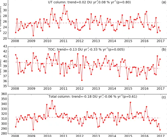
vations and in situ measurements (Gaudel et al., 2018). The conclusions in Sect. 3 show that no retrieval drift or instru-mental instability has been noticed that could explain the ob-served trend. It is worth noting that the trend derived from the IASI-B instrument for this second period is in agreement with the one reported here (see Sect. 3). In order to evaluate if the LT columns can be strongly contaminated by higher altitudes in the troposphere and the stratosphere, we also de-rive the trends for different partial columns: the upper tro-pospheric column (UT), ranging from 6 to 12 km, the tropo-spheric ozone column (TOC), ranging from the surface up to the tropopause, and the total column. Note that the UT column can include part of the lower stratosphere when the tropopause is lower than 12 km. The deseasonalized time se-ries are plotted in Fig. 7 with the derived trends indicated in the figure. The UT and total columns do not show any trend, whereas the TOC column presents a significant nega-tive trend that is likely driven by the neganega-tive trend observed in the lower troposphere. These results show that the negative trend observed in the lower troposphere with IASI is likely representative of the ozone evolution within the lower and (more likely) the free troposphere (3–5 km) where the IASI retrieval is the most sensitive. In the following, we explore the processes that could explain the ozone decrease observed in the LT from IASI in the NCP region. Several concomitant processes could explain the observed variability and trends: (i) recent studies show that several dynamical processes such as the QBO (quasi-biennial oscillation), ENSO (El Niño– Southern Oscillation), and STE (stratospheric–tropospheric exchange) influence the variability and trends of the tropo-spheric ozone column (e.g., Ebojie et al., 2016; Heue et al., 2016; Oman et al., 2013; Wespes et al., 2016, 2017, 2018). The long-range transport of ozone or precursors could also

influence regional LT ozone by advection; (ii) intensive emis-sion regulations have been applied in China to reduce SO2

and NOx emissions over roughly the last decade (van der A

et al., 2017; Li et al., 2017). The emission reduction of NOx

species, which are ozone precursors, has been observed in the satellite NO2columns since 2013, as shown in Fig. 8 and

reported in very recent inventories (Zheng et al., 2018). On the contrary, the emissions of anthropogenic volatile organic compounds (VOCs) are not regulated and do not show any decrease in recent years. Zheng et al. (2018) report an in-crease between 2010 and 2014 and stagnation since 2014. Stavrakou et al. (2017) report on an increase in 2013 and 2014 compared to previous years from OMI HCHO-based emissions and attribute it to the economic recovery after the 2008–2009 crisis. Looking at the time series of the HCHO tropospheric columns derived from OMI (De Smedt et al., 2015), available from the TEMIS database, a continuous in-crease is observed starting in 2013 and extending to 2016 (Fig. 8). It is worth noting that the increase is less observable in a more recent version of the HCHO product, except for the last year (De Smedt et al., 2018). Thus, one hypothesis is that reductions in the surface emissions of NOx and the

increase or stagnation in VOCs emissions might cause a de-creasing trend in lower tropospheric ozone levels as observed with IASI (Figs. 7–8).

4.2 Role of NOxemission reduction

In order to evaluate the impact of emission reduction on ozone, we first use the surface measurements made at the Shangdianzi station, China. The Shangdianzi station is a re-gional Global Atmosphere Watch (GAW) station, located about 100 km northeast of Beijing and is classified as a rural

Figure 6. Monthly, annual, and seasonal evolution of LT ozone over the NCP between 2008 and 2016 derived from IASI-A. (a) Monthly time series, (b) annual time series, (c) anomalies, (d) interannual variation of seasonal means, and (e) deseasonalized monthly time series with linear regression calculated for the 2008–2016 period (red), the 2008–2012 period (black), and the 2013–2016 period (green). The 2013 breakpoint of the deseasonalized time series (e) is chosen according to the significant change noticed in the annual time series (b) (see text for details).

station. Previous studies suggest that the pollutant observa-tions at this station are representative of the regional-scale air quality of the NCP (Lin et al., 2008; Xu et al., 2009) and are therefore more comparable to satellite observations than urban stations. Recent studies show a positive trend for surface ozone levels in the NCP (Ma et al., 2016; Sun et al., 2016). The time series are plotted in Fig. 9a, b for the 2009–2015 period. The calculated trend based on the desea-sonalized time series is positive at 0.31 ± 0.18 ppb yr−1 or 0.80±0.46 % yr−1. However, the trend is only slightly signif-icant over this time period as p = 0.09. We compare the sur-face measurements to the IASI LT columns, converted into equivalent volume mixing ratios. IASI observations within a

0.25◦×0.25◦area around the stations are considered (40.5– 40.75◦N, 117–117.25◦E). Considering all the surface data (daily, hourly), the linear trend calculated from the deseason-alized time series for the surface station (Fig. 9a, b) is pos-itive (slightly significant, p = 0.09), whereas the IASI trend (calculated for clear-sky days only) is significantly negative. Obviously, the quantities are not completely comparable as we compare columns and surface measurements and as IASI is poorly sensitive to the surface (Cuesta et al., 2018). IASI observations are made during the day and are more represen-tative of the free troposphere or of highly developed plane-tary boundary layers (PBL) (Eremenko et al., 2008); there-fore, they can not be compared to nighttime observations

16450 G. Dufour et al.: Lower tropospheric ozone over the North China Plain: variability and trends

Figure 7. Deseasonalized monthly time series of the upper tropospheric (UT) ozone column (a), the tropospheric ozone column (TOC, b), and the total ozone column (c).

when the PBL is isolated from the free troposphere. Hence, we only consider daytime (08:00–20:00 LT – local time) sur-face observations, which should be more representative of IASI observations. The calculated linear trend of the day-time surface measurement is still positive, but reduces and becomes poorly significant with a p value of 0.74 (Fig. 9c, d). Next, we consider daytime surface observations only on the days for which IASI data are available. The calculated linear trend becomes negative (not significant, Fig. 9f). We also consider the surface measurement the day after the IASI data are available. A recent study shows that the downward mixing of free tropospheric ozone may largely impact the morning level of ozone in the surface layer, with the surface ozone level on one day likely being related to ozone at higher levels the day before (Wang et al., 2017a). In that case, the calculated trend is even more negative but still poorly signif-icant (Fig. 9h). These results illustrate the sensitivity of the trend calculation to the sampling (day/night, clear-sky con-ditions) and stress the need to compare datasets with differ-ent temporal sampling frequencies over subsets of data with consistent sampling before drawing conclusions. In addition, the answers given by the surface and satellite observations are inconsistent: surface measurements show positive and/or non-significant trends and satellite observations show a sig-nificant negative trend. If both trends are reliable, a

possi-ble explanation for this inconsistency may be that the LT and surface ozone respond differently to the recent reduc-tion of NOx. Previous ozone production efficiency studies

(Ge et al., 2010, 2012) suggest that even at the background site of the NCP, ozone production in the surface layer seems to be more VOC-limited. Although Chinese NOxemissions

have been reduced in recent years, VOC emissions have been increasing or stagnating as previously mentioned. The ob-served recent decline of tropospheric NO2 (Fig. 8) might

have mainly contributed to the decrease of ozone at levels above the surface layer, where ozone production is more sen-sitive to NOx. To better understand the changes in ozone at

different altitudes over the NCP, we utilize simulation ex-periments from the chemistry transport model CHIMERE (Menut et al., 2013) made in the framework of another study (Lachâtre et al., 2018). Two runs of CHIMERE with dif-ferent emissions are compared for the year 2015. The first was performed based on the EDGAR-HTAP v2.2 2010 emis-sion inventory (Janssens-Maenhout et al., 2015) and is con-sidered as the reference case. For the second run, the SO2

and NO2 OMI tropospheric columns were used to update

the SO2 and NOx emissions using a simple mass balance

method for the emission correction. The corrected emissions then include the recent reduction of NOx emissions, which

Figure 8. Yearly moving averages of the deseasonalized time series of OMI NO2tropospheric columns (a), IASI LT ozone columns (b), and

OMI HCHO tropospheric columns (c) over the NCP. The thinner lines represent the 1σ standard deviation range of the moving averages.

the same for the two simulations. Figure 10 shows the differ-ences (as percentages) between the annual mean ozone con-centration simulated with updated emissions and with the ref-erence case at the surface and at ∼ 4 km. At the surface, the ozone concentrations simulated with reduced NOxemissions

are 13 % larger on average over the NCP. This corroborates the reported ozone increase, associated with the NOx

emis-sion reduction. On the contrary, the ozone concentrations at 4 km decrease compared to the reference when NOx

emis-sions are reduced. The impact is small, −0.25 % on average over the NCP but it persists in the altitude range between 3 and 7 km, which is the range where the IASI observations are the most sensitive. These results suggest that our hy-pothesis concerning the response of LT or free tropospheric ozone (decrease) to the NOxreduction is credible and likely

associated with the chemical regime changing from VOC-limited in the boundary layer to NOx-limited in the free

tro-posphere. However, quantifying the change of the chemical regime with the altitude is outside the scope of this study and would require observations with a better vertical resolu-tion than those offered by satellite observaresolu-tions, such as those from the IAGOS program (Petzold et al., 2015) and detailed model studies. The changes due to the NOx emission

reduc-tion on free tropospheric ozone remain small (Fig. 10) and do

not solely explain the negative trend observed with IASI. In the next section, we explore the processes contributing to the ozone variability and trend in addition to the NOx emission

reduction.

4.3 Explicative variables

The multivariate linear regression model described in Sect. 2 was used to determine the explicative variables of the nega-tive trend observed by IASI in the LT. The model has been applied for the entire 2008–2016 period but also for the 2013–2016 period for which the negative trend is the most significant. As the study focuses on the trend explanation, we applied the model to 3-month moving-average (deseasonal-ized) time series, with the month-to-month variations pos-sibly being more affected by the IASI sampling limited to clear-sky conditions. After the first application of the regres-sion model to determine the significant explicative variables as described in Sect. 2, we applied the model introducing the variables one by one. In order to evaluate the fit we calcu-lated (using the Theil–Sen estimator) the trend of fit residual, referred to as residual trend in the following, as well as the standard deviation of the residual. The results are reported in Table 2 for the two time periods studied.

16452 G. Dufour et al.: Lower tropospheric ozone over the North China Plain: variability and trends

Figure 9. Evolution of the time series (deseasonalized or not deseasonalized) when changing the sampling. The IASI equivalent column concentrations are plotted in black, and the surface concentrations measured at Shangdianzi station, China, are plotted in red.

Table 2. Evolution of the residual trend, and the contribution of the explicative variables to the observed trend.

2008–2016 2013–2016

Variables included in the fit Residual trend Contribution to Variables included in the fit Residual trend Contribution to (DU yr−1) the observed (DU yr−1) the observed

trend (%) trend (%)

Observed trend −0.17 Observed trend −0.29

QBO −0.15 12 QBO −0.26 10

QBO + PV −0.11 24 QBO + ENSO −0.18 28 QBO + PV + ENSO −0.08 18 QBO + ENSO + PV −0.15 10 QBO + PV + ENSO + CO −0.06 12 QBO + ENSO + PV + NO2 −0.04 38

Figure 10. Relative difference (%) at the surface (left) and at ∼ 4 km (right) between a CHIMERE simulation based on corrected NOxand

SO₂emissions using OMI satellite data and a CHIMERE simulation based on the EDGAR-HTAP-v2.2 2010 emission inventory.

Figure 11. Normalized explanatory variable time series between 2008 and 2016.

After the fitting procedure, the significant variables for the 2008–2016 period are the QBO, the potential vorticity (PV) at 300 hPa, the ENSO index, and the CO total columns de-seasonalized time series derived from IASI. The normalized time series are displayed in Fig. 11. The QBO mainly ac-counts for the low frequency variations and shows high sig-nificance (p<10−3), but it only explains 12 % of the initial trend (Table 2). The potential vorticity (PV) at 300 hPa was chosen in order to account for the impact of stratospheric– tropospheric exchanges on the LT ozone. A significant de-crease and trend are observed in the PV time series for the 2008–2016 period (Fig. 11), which allows one to explain 24 % of the decreasing trend observed with IASI in the LT

ozone. The normalized ENSO index shows an increase over the 2008–2016 period with two specific periods correspond-ing to two strong El Niño events in 2009–2010 and 2015– 2016. Introducing the ENSO index in the fit allows one to explain 18 % of the initial trend (Table 2). The last signifi-cant variable we found for this period was the monthly CO. The CO variable, due to its long lifetime, is considered to be a proxy for large-scale emission changes that may regionally affect LT ozone. To account for the long-range transport and advection, the regression model was tested either with the CO time series averaged for the Northern Hemisphere or with the CO time series averaged only over the NCP. Considering the CO averaged over the NCP leads to larger reduction of the

16454 G. Dufour et al.: Lower tropospheric ozone over the North China Plain: variability and trends

residual trend (12 % against 6 %) and suggests that regional and hemispheric changes can both slightly influence the LT ozone trend. During the 2008–2016 period, the dynamical processes such as the QBO, ENSO, and the STE seem to be the main drivers of the trend observed with IASI. The re-gional and hemispheric emission changes approximated by CO only contribute slightly (12 %). Among the significant explicative variables, the PV, which also shows a decrease during the 2008–2016 period, is the explicative variable con-tributing the most to the calculated linear trend. This points toward a possible reduction of the stratospheric–tropospheric exchanges that leads to a reduction of ozone levels in the free/lower troposphere. However, the different explicative variables only explain 65 % of the observed trend. The resid-ual trend remains significant and as high as −0.06 DU yr−1. Therefore, including an additional trend in the fit is necessary in order to come up with a negligible non-significant residual trend (0.005 DU yr−1; Table 2). Thus, explicative variables to fully explain the decreasing trend observed with IASI are still missing. One hypothesis to explain this concerns the lim-itation of the linear regression model regarding its ability to account for nonlinear processes, such as the chemistry driv-ing the ozone production.

Concerning the 2013–2016 period, the significant vari-ables are the QBO, the PV at 300 hPa, the ENSO index, the NO2tropospheric columns, and the HCHO tropospheric

columns. As previously discussed, the QBO, the PV, and the ENSO variables indicate the role of large-scale dynamical processes, whereas the NO2 and HCHO variables indicate

the role of chemistry and source reduction. Accounting for these variables, 90 % of the negative trend observed with IASI between 2013 and 2016 is explained. The ENSO in-dex with the large El Niño events in 2015–2016 as well as the decline of the NO2 tropospheric columns are the main

contributions, 28 % and 38 %, respectively, to explain the trend. Note that the residual trend is not significant and no additional trend is necessary. We did the test of introduc-ing an additional trend but it does not reduce the residual trend, and the p value associated with the additional trend is very large (0.55). For the shorter time period from 2013 to 2016, when the variations of the explicative variables are monotone, especially for NO2(Fig. 8), the linear regression

model succeeds in explaining most of the observed trend. In this case, the regression model results suggest that dynami-cal processes as well as emission reduction contribute almost equally to the decreasing trend observed by IASI in the LT.

5 Conclusions

We use the IASI-A instrument to calculate the trends of LT ozone over the NCP during the 9-year period from 2008 to 2016. However, questions remain regarding the reliability of a tropospheric ozone trend derived from satellite observa-tions. Indeed, a recent study comparing tropospheric ozone

trends derived from IR and UV satellite sounders has re-veal inconsistencies (Gaudel et al., 2018), with IR sounders showing a general negative trend (Oetjen et al., 2016; We-spes et al., 2018) and UV sounders displaying a general positive trend (Cooper et al., 2014). The first step of our study was then to evaluate the stability and the reliability of the IASI ozone product used to calculate the trend. On one hand, we explored the temporal evolution of the inter-nal and exterinter-nal parameters that the retrieval is sensitive to; on the other hand, we compared the IASI-A ozone observa-tions with independent measurements. As thermal infrared observations are sensitive to the atmospheric thermal con-ditions, we evaluated the temporal evolution of the surface temperature and the thermal contrast over the NCP between 2008 and 2016. No specific or significant trend was found. We also explored the influence of the changes in tropopause height on the LT ozone columns. No significant trend was noticed in the tropopause height during the study period. Coarse aerosol spectral features can contaminate the ozone spectral region used for the retrieval and, in turn, possibly affect the ozone retrieval. Filtering out observations associ-ated with large aerosol loading (AOD > 0.2) does not signif-icantly change the calculated trend from IASI observations. Thus, large aerosol loading that regularly occurs over China does not impact the trend derived from IASI. The stability of the retrieval was evaluated using the AK and the asso-ciated parameters: the DOF and the altitude of maximum sensitivity. These two parameters do not show any signif-icant trend. In addition, we performed a numerical experi-ment by considering a 9-year period with a constant ozone profile (and thus no trend). We applied the AK to the pro-file to evaluate the capability of the IASI ozone product used to reproduce this no-trend situation. No significant trend has been found in the resulting time series. Finally, we compared the LT ozone columns derived from IASI-A to independent observations. Comparison with the independent IASI-B ob-servations over the 2013–2016 period shows similar trends. This indicates that instrumental drift is not responsible for the trend calculated from IASI-A observations. Comparisons with Asian ozonesondes show a bias ranging from −10 % to −15 %. The limited sampling and changes in the instru-mentation of three out of five sondes during the study period do not allow one to clearly evaluate and make firm conclu-sions concerning the reliability of IASI trends compared with those of the sondes. In general, comparisons with indepen-dent measurements (sondes or surface in situ) performed in this study show the importance of the sampling regarding the conclusions drawn. Differences in the sampling can signifi-cantly affect the trends calculated and thus the conclusions. One recommendation when comparing datasets with differ-ent sampling parameters would be to perform the comparison over subsets of data with similar sampling methods.

According to the evaluation carried out, the trends derived from the IASI-A observations seem fairly reliable and can be used to study the LT ozone trend over the NCP. The analysis

of the LT ozone columns shows a negative trend for ozone in the lower troposphere with 2013 being a pivotal year. Be-fore 2013, no trend is detected, whereas a significant nega-tive trend of −0.24 ± 0.06 DU yr−1(−1.161 ± 0.003 % yr−1) is derived for the 2013–2016 period. A similar trend is ob-served with the independent IASI-B instrument for the same period. Comparison with trends calculated for other partial columns (UT and TOC) shows that the trend derived for the LT is independent of other partial columns and well represen-tative of the LT or more specifically of the free troposphere (3–5 km) where the IASI ozone product used is the most sen-sitive. We use a multivariate linear regression model to iden-tify the processes driving the observed trend. The results sug-gest that both large-scale dynamical processes and regional emission changes explain the trend. At the end of the period (2013–2016), both factors contribute almost equally to the observed trends with the strong ENSO event in 2015–2016 and NOx emission reduction being the largest contributors.

For the entire period (2008–2016), the dynamical processes, especially a possible reduction of the STE, dominate to plain the 9-year trend. However, the entire trend is not ex-plained by the linear regression model highlighting the diffi-culty of identifying good proxies to characterize the role of advection and long-range transport and to account for nonlin-ear processes such as ozone chemistry. To properly evaluate these processes, the use of chemistry transport models is cer-tainly needed; however, it is challenging to have updated and consistent emissions for all of the co-emitted species over the entire hemisphere for a time period covering about 10 years. For example, using the CHIMERE model, we have been able to evaluate the response of ozone to the NOx emissions

re-duction, which is different depending on the altitude (pos-itive in the boundary layer and negative above 3 km). This explains, at least partly, the apparent inconsistency between the positive trend derived from the surface measurements and the negative trend derived in the lower/free troposphere from IASI. A better understanding and evaluation of the altitude-dependent ozone response to emission changes and the link with chemical regimes are still necessary. Therefore, detailed modeling studies such as the one reported by Jin et al. (2017) but extended in altitude are necessary and require observa-tions with a high vertical resolution, such as those provided by aircraft campaigns or the IAGOS program (Petzold et al., 2015).

Code and data availability. The IASI observations (level 1C) are available from the AERIS data infrastructure (http://www. aeris-data.fr/, last access: November 2018). The IASI ozone prod-uct retrieved from the level 1C data is available, upon requested from Gaëlle Dufour (dufour@lisa.u-pec.fr), for the Asian domain considered in this study between 2008 and 2016.

The NO2and HCHO tropospheric columns from OMI are

avail-able at http://www.temis.nl (last access: November 2018).

The ozonesonde data are available from the WOUDC database (https://woudc.org/, last access: November 2018), except for the Beijing station. These data can be requested directly from the PI of the station, Yi Liu (liuyi@mail.iap.ac.cn). The surface measure-ments at the SDZ station are available upon request from the PIs of the station, Xiaobin Xu (13311298991@189.cn) and Weili Lin (linwl@muc.edu.cn).

The CHIMERE model is publicly available at http://www.lmd. polytechnique.fr/chimere/ (Menut, 2013).

Author contributions. GD managed the study (from its concep-tion), the formal analysis of data, the preparation of the paper, and the funding acquisition. ME performed the IASI ozone retrieval and managed the resulting level-2 product. MB, JC, and GF participated in the conception of the study and in reviewing and editing the pa-per. AFC and ML performed the model simulations and the emis-sion corrections. WL and XX provided the surface observations, participated in the analysis, and reviewed the paper. YL and YZ provided the ozonesonde measurements over Beijing and support regarding their analysis; they also reviewed the paper.

Competing interests. The authors declare that they have no conflict of interest.

Acknowledgements. The authors are grateful for the essential support from the Agence Nationale de la Recherche (ANR) through the PolEASIA project (ANR-15-CE04-0005). The IASI mission is a joint mission of EUMETSAT and the Centre National d’Etudes Spatiales (CNES, France). This study was financially supported by the French Space Agency – CNES (project “IASI/TOSCA”). The authors acknowledge the AERIS data infrastructure (https://www.aeris-data.fr, last access: August 2018) for providing access to the IASI Level 1C data, distributed in near-real-time by EUMETSAT through the EUMETCast system distribution. The authors acknowledge the dataset producers and providers of data used in this study: the LATMOS/ULB for the provision of the IASI CO total columns through the AERIS database; the ozonesonde data used in this study were mainly provided by the World Ozone and Ultraviolet Data Centre (WOUDC) and are publicly available (see http://www.woudc.org, last access: August 2018); the NASA Giovani portal for access to the MODIS AOD products; and the ERA-Interim portal for access to the meteorological fields needed to support our study. We acknowledge the Institut für Meteorologie und Klimaforschung (IMK), Karlsruhe, Germany, for the licence to use the KOPRA radiative transfer model. We also warmly thank Owen R. Cooper from NOAA (US) for his support and fruitful discussions as well as Didier Hauglustaine from LSCE (France) for providing the LMDZ-INCA model simulations.

Edited by: Michel Van Roozendael Reviewed by: two anonymous referees

16456 G. Dufour et al.: Lower tropospheric ozone over the North China Plain: variability and trends References

Boersma, K. F., Eskes, H. J., Veefkind, J. P., Brinksma, E. J., van der A, R. J., Sneep, M., van den Oord, G. H. J., Levelt, P. F., Stammes, P., Gleason, J. F., and Bucsela, E. J.: Near-real time retrieval of tropospheric NO2from OMI, Atmos. Chem. Phys.,

7, 2103–2118, https://doi.org/10.5194/acp-7-2103-2007, 2007. Boynard, A., Hurtmans, D., Koukouli, M. E., Goutail, F., Bureau,

J., Safieddine, S., Lerot, C., Hadji-Lazaro, J., Wespes, C., Pom-mereau, J.-P., Pazmino, A., Zyrichidou, I., Balis, D., Barbe, A., Mikhailenko, S. N., Loyola, D., Valks, P., Van Roozendael, M., Coheur, P.-F., and Clerbaux, C.: Seven years of IASI ozone re-trievals from FORLI: validation with independent total column and vertical profile measurements, Atmos. Meas. Tech., 9, 4327– 4353, https://doi.org/10.5194/amt-9-4327-2016, 2016.

Boynard, A., Hurtmans, D., Garane, K., Goutail, F., Hadji-Lazaro, J., Koukouli, M. E., Wespes, C., Vigouroux, C., Keppens, A., Pommereau, J.-P., Pazmino, A., Balis, D., Loyola, D., Valks, P., Sussmann, R., Smale, D., Coheur, P.-F., and Clerbaux, C.: Validation of the IASI FORLI/EUMETSAT ozone products us-ing satellite (GOME-2), ground-based (Brewer-Dobson, SAOZ, FTIR) and ozonesonde measurements, Atmos. Meas. Tech., 11, 5125–5152, https://doi.org/10.5194/amt-11-5125-2018, 2018. Chen, X., Huang, F. X., Xia, X. Q., Cao, J., and Xu, X.:

Analy-sis of tropospheric ozone long-term changing trends and affect-ing factors over northern China, Chin. Sci. Bull., 60, 2659–2666, https://doi.org/10.1360/N972015-00155, 2015 (in Chinese). Clerbaux, C., Boynard, A., Clarisse, L., George, M., Hadji-Lazaro,

J., Herbin, H., Hurtmans, D., Pommier, M., Razavi, A., Turquety, S., Wespes, C., and Coheur, P.-F.: Monitoring of atmospheric composition using the thermal infrared IASI/MetOp sounder, At-mos. Chem. Phys., 9, 6041–6054, https://doi.org/10.5194/acp-9-6041-2009, 2009.

Cooper, O. R., Parrish, D. D., Ziemke, J., Balashov, N. V., Cu-peiro, M., Galbally, I. E., Gilge, S., Horowitz, L., Jensen, N. R., Lamarque, J.-F., Naik, V., Oltmans, S. J., Schwab, J., Shindell, D. T., Thompson, A. M., Thouret, V., Wang, Y., and Zbinden, R. M.: Global distribution and trends of tropospheric ozone: An observation-based review, Elem. Sci. Anthr., 2, 2:000029, https://doi.org/10.12952/journal.elementa.000029, 2014. Cuesta, J., Kanaya, Y., Takigawa, M., Dufour, G., Eremenko, M.,

Foret, G., Miyazaki, K., and Beekmann, M.: Transboundary ozone pollution across East Asia: daily evolution and photo-chemical production analysed by IASI + GOME2 multispec-tral satellite observations and models, Atmos. Chem. Phys., 18, 9499–9525, https://doi.org/10.5194/acp-18-9499-2018, 2018. De Smedt, I., Stavrakou, T., Hendrick, F., Danckaert, T.,

Vlem-mix, T., Pinardi, G., Theys, N., Lerot, C., Gielen, C., Vigouroux, C., Hermans, C., Fayt, C., Veefkind, P., Müller, J.-F., and Van Roozendael, M.: Diurnal, seasonal and long-term variations of global formaldehyde columns inferred from combined OMI and GOME-2 observations, Atmos. Chem. Phys., 15, 12519–12545, https://doi.org/10.5194/acp-15-12519-2015, 2015.

De Smedt, I., Theys, N., Yu, H., Danckaert, T., Lerot, C., Comper-nolle, S., Van Roozendael, M., Richter, A., Hilboll, A., Peters, E., Pedergnana, M., Loyola, D., Beirle, S., Wagner, T., Eskes, H., van Geffen, J., Boersma, K. F., and Veefkind, P.: Algorithm theo-retical baseline for formaldehyde retrievals from S5P TROPOMI and from the QA4ECV project, Atmos. Meas. Tech., 11, 2395– 2426, https://doi.org/10.5194/amt-11-2395-2018, 2018.

Ding, A. J., Wang, T., Thouret, V., Cammas, J.-P., and Nédélec, P.: Tropospheric ozone climatology over Beijing: analysis of aircraft data from the MOZAIC program, Atmos. Chem. Phys., 8, 1–13, https://doi.org/10.5194/acp-8-1-2008, 2008.

Dufour, G., Eremenko, M., Orphal, J., and Flaud, J.-M.: IASI observations of seasonal and day-to-day variations of tropo-spheric ozone over three highly populated areas of China: Bei-jing, Shanghai, and Hong Kong, Atmos. Chem. Phys., 10, 3787– 3801, https://doi.org/10.5194/acp-10-3787-2010, 2010. Dufour, G., Eremenko, M., Griesfeller, A., Barret, B.,

LeFlochmoën, E., Clerbaux, C., Hadji-Lazaro, J., Coheur, P.-F., and Hurtmans, D.: Validation of three different scientific ozone products retrieved from IASI spectra using ozonesondes, Atmos. Meas. Tech., 5, 611–630, https://doi.org/10.5194/amt-5-611-2012, 2012.

Dufour, G., Eremenko, M., Cuesta, J., Doche, C., Foret, G., Beek-mann, M., Cheiney, A., Wang, Y., Cai, Z., Liu, Y., Takigawa, M., Kanaya, Y., and Flaud, J.-M.: Springtime daily variations in lower-tropospheric ozone over east Asia: the role of cyclonic ac-tivity and pollution as observed from space with IASI, Atmos. Chem. Phys., 15, 10839–10856, https://doi.org/10.5194/acp-15-10839-2015, 2015.

Ebojie, F., Burrows, J. P., Gebhardt, C., Ladstätter-Weißenmayer, A., von Savigny, C., Rozanov, A., Weber, M., and Bovensmann, H.: Global tropospheric ozone variations from 2003 to 2011 as seen by SCIAMACHY, Atmos. Chem. Phys., 16, 417–436, https://doi.org/10.5194/acp-16-417-2016, 2016.

Eremenko, M., Dufour, G., Foret, G., Keim, C., Orphal, J., Beek-mann, M., Bergametti, G., and Flaud, J. M.: Tropospheric ozone distributions over Europe during the heat wave in July 2007 ob-served from infrared nadir spectra recorded by IASI, Geophys. Res. Lett., 35, 0–4, https://doi.org/10.1029/2008GL034803, 2008.

Gaudel, A., Cooper, O. R., Ancellet, G., Barret, B., Boynard, A., Burrows, J.P., Clerbaux, C., Coheur, P.-F., Cuesta, J., Cuevas, E., Doniki, S., Dufour, G., Ebojie, F., Foret, G., Garcia, O., Grana-dos Muños, M. J., Hannigan, J. W., Hase, F., Huang, G., Hassler, B., Hurtmans, D., Jaffe, D., Jones, N., Kalabokas, P., Kerridge, B., Kulawik, S. S., Latter, B., Leblanc, T., Le Flochmoën, E., Lin, W., Liu, J., Liu, X., Mahieu, E., McClure-Begley, A., Neu, J. L., Osman, M., Palm, M., Petetin, H., Petropavlovskikh, I., Querel, R., Rahpoe, N., Rozanov, A., Schultz, M. G., Schwab, J., Sid-dans, R., Smale, D., Steinbacher, M., Tanimoto, H., Tarasick, D. W., Thouret, V., Thompson, A. M., Trickl, T., Weatherhead, E., Wespes, C., Worden, H. M., Vigouroux, C., Xu, X., Zeng, G., and Ziemke, J.: Tropospheric Ozone Assessment Report: Present-day distribution and trends of tropospheric ozone relevant to climate and global atmospheric chemistry model evaluation, Elem. Sci. Anth., 6, p. 39, https://doi.org/10.1525/elementa.291, 2018 Ge, B., Xu, X., Lin, W., and Wang, Y.: Observational Study of

Ozone Production Efficiency at the Shangdianzi Regional Back-ground Station, Chinese J. Environ. Sci., 31, 1444–1450, 2010. Ge, B. Z., Xu, X. B., Lin, W. L., Li, J., and Wang, Z. F.: Impact of

the regional transport of urban Beijing pollutants on downwind areas in summer: ozone production efficiency analysis, Tellus B, 64, 17348, https://doi.org/10.3402/tellusb.v64i0.17348, 2012. George, M., Clerbaux, C., Hurtmans, D., Turquety, S., Coheur,

P.-F., Pommier, M., Hadji-Lazaro, J., Edwards, D. P., Worden, H., Luo, M., Rinsland, C., and McMillan, W.: Carbon monoxide