HAL Id: hal-02453884
https://hal.archives-ouvertes.fr/hal-02453884
Submitted on 10 Nov 2020
HAL is a multi-disciplinary open access
archive for the deposit and dissemination of
sci-entific research documents, whether they are
pub-lished or not. The documents may come from
teaching and research institutions in France or
abroad, or from public or private research centers.
L’archive ouverte pluridisciplinaire HAL, est
destinée au dépôt et à la diffusion de documents
scientifiques de niveau recherche, publiés ou non,
émanant des établissements d’enseignement et de
recherche français ou étrangers, des laboratoires
publics ou privés.
On the Link Between External Forcings and Slope
Instabilities in the Piton de la Fournaise Summit Crater,
Reunion Island
Virginie Durand, Anne Mangeney, Florian Haas, Xiaoping Jia, Fabian Bonilla,
Aline Peltier, Clément Hibert, Valérie Ferrazzini, Philippe Kowalski, Fréderic
Lauret, et al.
To cite this version:
Virginie Durand, Anne Mangeney, Florian Haas, Xiaoping Jia, Fabian Bonilla, et al.. On the Link
Between External Forcings and Slope Instabilities in the Piton de la Fournaise Summit Crater, Reunion
Island. Journal of Geophysical Research: Earth Surface, American Geophysical Union/Wiley, 2018,
123 (10), pp.2422-2442. �10.1029/2017JF004507�. �hal-02453884�
On the Link Between External Forcings and Slope Instabilities
in the Piton de la Fournaise Summit Crater, Reunion Island
Virginie Durand1 , Anne Mangeney1, Florian Haas2 , Xiaoping Jia3, Fabian Bonilla1,4 ,
Aline Peltier5 , Clément Hibert6 , Valérie Ferrazzini5 , Philippe Kowalski5, Frédéric Lauret5,
Christophe Brunet5, Claudio Satriano1 , Kerstin Wegner2, Arthur Delorme1 , and
Nicolas Villeneuve5
1Institut de Physique du Globe de Paris, CNRS UMR 7154, Université Paris Diderot-Paris 7, Paris, France,2Catholic University of Eichstaett-Ingolstadt, Eichstätt, Germany,3Institut Langevin, ESPCI Paris Tech, CNRS UMR 7587, Paris, France, 4IFSTTAR, Université Paris-Est, Paris, France,5Observatoire Volcanologique du Piton de la Fournaise/Institut de Physique du Globe de Paris, Sorbonne Paris Cité, La Plaine des Cafres, Réunion Island, France,6Institut de Physique du Globe de Strasbourg, EOST, UMR 7516 CNRS, Strasbourg, France
Abstract
We have analyzed the impact of different forcings, such as rain and seismicity, on slope instabilites on an active volcano. For this, we compiled a catalog of the locations and volumes of rockfalls in the Piton de la Fournaise crater using seismic records. We validated it by comparing the locations and volumes to those deduced from photogrammetric data. We analyzed 10,477 rockfalls, spanning the period 2014 to 2016. This period corresponds to the renewal of volcanic activity after a 41-month rest. Our analysis reveals that renewed eruptive activity has unsettled the crater edges. External forcings such as rain and seismicity are shown to potentially increase the number and the volume of rockfalls, with a stronger impact on the volume. Preeruptive seismicity seems to be the main triggering factor for the largest volumes, with a delay of one to several days. Rain alone does not seem to trigger especially large rockfalls. We infer that repetitive vibrations from the many seismic events, combined with the action of rain, induce crack (or slip) growth in highly fractured (or granular) materials, leading to the collapse of large volumes. Regarding their spatial distribution before an eruption, the largest rockfalls seem to migrate toward the location of magma extrusion.1. Introduction
Rockfalls (RFs) form one of the main geomorphic processes involved in the reshaping of landscapes in moun-tainous areas (De Blasio, 2011). Because of their sudden and often unpredictable occurrences, they represent an important natural hazard. RFs are mainly controlled by different external factors, such as climate (D’Amato et al., 2016; Delonca et al., 2014; Dietze, Mohadjer, et al., 2017; Helmstetter & Garambois, 2010; Krautblatter et al., 2012), seismicity (Keefer, 2002; Lin et al., 2008; Tatard et al., 2010), and volcanic activity (Calder et al., 2002; Hibert, Mangeney, et al., 2017; Voight et al., 2000). However, the influence of these factors and the way they trigger RFs are not yet well understood (D’Amato et al., 2016; Dietze, Turowski, et al., 2017; Hibert, Mangeney, et al., 2017; Stock et al., 2013). Indeed, it is difficult to clearly link these different forcings to RF occurrences. One reason is that these different forcings can overlap or have additive effects. Another is that time-accurate data are needed to better constrain the relationship between the triggers and the RFs. Until recently, RFs were only identified and classified using field observations or aerial/satellite images (Krautblatter et al., 2012; Lacroix, 2016). This leads to high uncertainty in their times of occurrence. New monitoring techniques, with regular photography and lidar campaigns or satellite data, can provide more complete catalogs of RFs in a given region (among others, Abellan et al., 2011; D’Amato et al., 2016; Lacroix, 2016). However, they do not provide accurate occurrence times, with time precision of tens of minutes in the case of continuous moni-toring, and sometimes give access only to the cumulative volume of several RFs. Over the last few years, in order to obtain more accurate RF catalogs, new methods have been developed to compute the volumes of RFs from seismic signals, in addition to detecting and locating them accurately (Dammeier et al., 2011; Deparis et al., 2008; Dietze, Mohadjer, et al., 2017; Helmstetter & Garambois, 2010; Hibert et al., 2011, 2014; Lacroix & Helmstetter, 2011; Norris, 1994; Zimmer & Sitar, 2015). These new catalogs, with precise occurrence times (pre-cision on the order of seconds) and location and volume of each individual event, allow more detailed studies
RESEARCH ARTICLE
10.1029/2017JF004507
Key Points:
• We investigate the link between external forcings and rockfall volume in a volcanic environment • We highlight delayed triggering of
large rockfalls by small repetitive seismic events
• We compare the rockfall volume estimated using seismic and photogrammetric data Supporting Information: • Supporting Information S1 Correspondence to: V. Durand, vdurand@ipgp.fr Citation:
Durand, V., Mangeney, A., Haas, F., Jia, X., Bonilla, F., Peltier, A., et al. (2018). On the link between external forcings and slope instabilities in the Piton de la Fournaise summit crater, Reunion Island. Journal of Geophysical
Research: Earth Surface, 123, 2422–2442.
https://doi.org/10.1029/2017JF004507
Received 9 OCT 2017 Accepted 3 SEP 2018
Accepted article online 17 SEP 2018 Published online 10 OCT 2018
©2018. American Geophysical Union. All Rights Reserved.
Journal of Geophysical Research: Earth Surface
10.1029/2017JF004507
on the links between RFs and external forcings like climate and seismic or volcanic activity (Dietze, Turowski, et al., 2017; Helmstetter & Garambois, 2010; Hibert, Mangeney, et al., 2017; Lacroix & Helmstetter, 2011). It is well known that rain can trigger RFs through several possible mechanisms. It can increase the pore pressure (Dietze, Turowski, et al., 2017), or it can produce chemical weathering, dissolving rock compounds (D’Amato et al., 2016; Dietze, Turowski, et al., 2017; Krautblatter et al., 2012). Whatever the process involved, RF activity has been shown to generally begin 1 hr to 2 days after the triggering rain episode (D’Amato et al., 2016; Delonca et al., 2014; Dietze, Turowski, et al., 2017; Helmstetter & Garambois, 2010; Krautblatter et al., 2012). Helmstetter and Garambois (2010) also point out that rain can have a long-lasting effect, with RF activ-ity continuing several days after the rain has stopped. Earthquakes are a second important triggering factor. Existing studies on the influence of earthquakes on slope instabilities mainly concern landslides or a mix of RFs and landslide events. They show that earthquakes can produce a permanent decrease in bulk ground strength leading to a slope collapse (Ambraseys & Bilham, 2012; Marc et al., 2015). This mechanism can explain why high landslide rates are observed for several months to years after an earthquake (Lin et al., 2008; Marc et al., 2015). The combination of seismic shaking and elevated pore pressure can lead to slope destabilization several days after ground shaking has stopped (Keefer, 2002). It is commonly assumed that earthquakes with magnitude M< 4 are not potential triggers for slope instabilities (Keefer, 1984; Tatard et al., 2010). However, some observations suggest that sequences of small seismic events (M< 3.6), because of repetitive shaking, may contribute to the triggering of a rockslide (Del Gaudio et al., 2000). Although it is difficult to clearly dis-criminate rain and earthquake effects in some regions (Lin et al., 2008; Tatard et al., 2010), during dry periods of the year, seismicity appears to be the most important triggering factor (Koukouvelas et al., 2015). A third important triggering factor is volcanic activity. It has been shown in several studies that volcanic seismicity, explosions due to eruptive activity, and local surface deformations due to magmatic intrusion and extrusion trigger RFs on volcanic edifices (Calder et al., 2002; Hibert, Mangeney, et al., 2017; Voight et al., 2000). These studies highlight the need for systematic data to improve the understanding of the role of external forcings, especially the influence of small seismicity, in slope destabilization. Here we apply the method devel-oped by Hibert et al.(2011, 2014) to investigate the spatiotemporal evolution of the number and volume of RFs in the crater of the Piton de la Fournaise volcano (Reunion Island). These RFs are subjected to rain, vol-canic seismicity, and deformation. We first explain how we create a catalog of RFs, comprising their occurrence dates, locations, and volumes, using the seismic signals they generate. We then validate these locations and volumes with those obtained from photogrammetric data. Next, we use our RF catalog to analyze the spa-tiotemporal evolution of RFs. We correlate them with external forcings such as seismic and eruptive activity and rainfall. In the last section, we discuss the links between the changes in RF activity and external forcings, in particular the influence of seismic activity and rainfall on the size of RFs.
2. Study Site
The Piton de la Fournaise volcano is a unique site to study RFs. The first reason is that the Dolomieu crater floor collapsed during the major April 2007 eruption (Michon et al., 2007; Peltier, Staudacher, et al.,2009; Staudacher et al., 2009), exposing mostly vertical rockwalls prone to a continuous RF activity. The second reason is that the summit of the volcano is densely instrumented, with seismic and geodetic networks (Figure 1), cameras, and regular photogrammetric campaigns. It thus offers an unparalleled combination of data to study RF activity. Finally, Piton de la Fournaise is located in a tropical region and is one of the most active basaltic volcanoes in the world, with an eruption every 8 months on average (Peltier, Bachèlery, et al. 2009; Roult et al., 2012; Staudacher et al., 2009). This setting makes it possible to investigate the influence of different kinds of forcings on RF activity, such as rainfall and seismic and volcanic activities.
Hibert et al., (2011, 2014, 2017) used the seismic network to analyze the RF activity that followed the 2007 Dolomieu summit crater collapse. They show that the highest RF activity lasted for 2 months after the col-lapse. This 2-month strong relaxation phase was followed by a smoother and longer phase exhibiting a constant rate of RFs but with a decrease in their volume. This phase lasted at least 3 years, until 2010 (Hibert et al., 2017), suggesting a long-term evolution of RF activity related to crater stability. They also analyzed the spatiotemporal evolution of RFs in the Dolomieu crater during this particularly active period, between 2007 and 2011. They observed an increase in the number and volume of RFs before some eruptions and the migration of the RFs toward the location of the next eruption, sometimes occurring 1 or 2 years later. This migration pattern is in agreement with the location of seismic noise changes observed before some eruptions
Figure 1. (a) Digital elevation model of the Piton de la Fournaise volcano and location of the seismic and Global
Navigation Satellite System (GNSS) stations used in this study and of the eruptions that occurred from 2014 to 2016. (1) 20 and 21 June 2014, (2) 4–15 February 2015, (3) 17–30 May 2015, (4) 30 July to 2 August 2015, (5) 24 August to 31 October 2015, (6) 26 and 27 May 2016, and (7) 11–18 September 2016. The lines next to the eruption numbers show the location of the eruptive fissures. (b) Piton de la Fournaise on Reunion island. The red box denotes the area shown in (a).
(Obermann et al., 2013). These changes highlight the existence of a mechanical forcing at depth linked to magma intrusion that may explain the observed migration of the RFs. However, because the 2007–2010 period was dominated by RF activity related to the crater collapse relaxation, it is difficult to clearly link RF activity with different external forcings such as rainfall and eruptive activity. To better assess the impact of the different forcings without the dominant influence of the postcollapse relaxation of the crater slopes, we analyze here the RF activity over a period long after the collapse, between 2014 and 2016. During this period, seven eruptions occurred, after a break that lasted 41 months. Looking at a period long after the crater col-lapse allows us to both confirm some results of Hibert et al. (2017) and highlight new links with the forcings (coupled action of seismicity and rain) that were hidden during the postcollapse relaxation period.
3. Materials and Methods
3.1. DataThe Piton de la Fournaise volcano is very well instrumented, with 39 seismic and 24 Global Navigation Satel-lite System (GNSS) stations. During the 2014–2016 study period, we consider only the four summit seismic stations and the six GNSS stations indicated in Figure 1. We use the seismic signals generated by RFs (see examples in Figure 2) at these four stations to locate the RFs. To compute their volumes, we use only three sta-tions (BOR, DSO, and SNE) because of the presence of strong site effects at BON station. BOR and DSO stasta-tions present a gap in the data from 17 February 2014 to 4 March 2014, leading to no volume estimation during this short period. GNSS stations are used to quantify the deformation of the cone. GNSS data are postprocessed with the GAMIT/GLOBK software package (Herring et al., 2010). GAMIT uses (i) the precise ephemerides of the international GNSS Service (IGS); (ii) a stable support network of 20 IGS stations not located on Reunion Island but scattered elsewhere in the Indian Ocean; (iii) a tested parameterization of the troposphere; and (iv) mod-els of ocean loading, Earth, and lunar tides. Plate motion used to correct data is deduced from the REUN IGS station located 15 km to the west of the summit and assumed not to be affected by any volcanic deformation. The final daily precision of the measurements is on the order of millimeters. Daily rain data are obtained from a rain gauge located at SNE station, at the summit of the cone.
Journal of Geophysical Research: Earth Surface
10.1029/2017JF004507
Figure 2. Examples of seismic signals generated by rockfalls of different volumes. The red and blue vertical bars show
the beginning and end of the rockfall signals, respectively, detected using the method proposed by Hibert et al. (2014). These signals were all recorded at DSO station.
Two lidar/photogrammetric campaigns were conducted at Piton de la Fournaise volcano. The first one was done in November 2014 and the second in January 2016. These measurements allow us to directly estimate the cumulative RF volume during this period and to compare it with the one computed from seismic data. 3.2. Detection, Classification, and Location of RFs Using Seismic Data
To extract the seismic signals corresponding to RFs at the four summit seismic stations (Figure 1), we use the RF catalog provided by the Observatoire Volcanologique du Piton de la Fournaise (OVPF). In the OVPF cata-log, events are classified manually, based on the knowledge and expertise of the operators. Thus, we apply the classification code developed by Hibert et al. (2014) on the extracted signals to remove potential signals that are not generated by RFs. The next step consists in picking the onset of the signal, using a kurtosis-based method (Baillard et al., 2014; Hibert et al., 2014). Then, we apply a locating method based on propagation models built using the Fast Marching Method (Hibert et al., 2014, Sethian, 1996a, 1996b, 1996c). For each pair of stations, it produces a hyperbola corresponding to the most probable source location based on the differ-ence between picked arrival times. For each event, all the hyperbola are stacked, their crossing point giving the optimal location of the source. The uncertainties in picking the signal onset and in the locating process are taken into account (supporting information Text S1), providing an estimation of the spatial location error. We keep only RFs with a location error of less than 500 m, which corresponds to the radius of the crater. 3.3. Volume Estimation Using Seismic Data
We compute the RF volume (Figure 3a) using the formula proposed by Hibert et al. (2011):
V = 3ES
RS∕P𝜌gL(tan 𝛿 cos 𝜃 − sin 𝜃),
(1) where𝜌 = c0𝜌iis the density of the granular mass, with the density of intact rock𝜌i= 2,000 kg/m3and the
solid volume fraction of the granular material c0 = 0.6. The length of the slope over which RFs occur L and
the slope angle𝜃 being fairly uniform all around the crater, we use fixed values: We choose L = 500 m as the average length and𝜃 = 35∘ as the mean slope angle. The 𝛿 = 0∘ is the repose angle of the deposit on the slope (the deposit is very flat, almost parallel to the slope), and RS∕Pis the mean ratio between seismic energy and potential energy lost by RFs.
We compute the seismic energy ESusing a formula proposed by Vilajosana et al. (2008): ES= ∫
t2
t1
Figure 3. (a) Volumes of the RFs (V1∕3is represented) that occurred from October 2014 to January 2016, computed using seismic signals. Each round dot represents a RF, and its radius and color are proportional to the cubic root of the RF volume. The white square defines the area where the total volume (100,000 m3) is computed. (b) Same as (a) but
using photogrammetric data and method. The dotted ellipse highlights the inferred subsiding zone. RF = rockfall.
where t1 and t2are, respectively, the picked onset and final times of the seismic signal, r is the distance between the event and the recording station, h = 160 m the thickness of the layer through which surface waves propagate, and𝜌 = 2,000 kg/m3the density of the ground. The𝛼 = f𝜋∕Qc is a damping factor that
accounts for anelastic attenuation of the waves (Aki & Richards, 1980), where f = 5 Hz is the frequency, Q = 50 the quality factor, and c the group velocity of surface waves, being the optimal velocity given by the locating method, ranging from 480 to 1,200 m/s. The uenv(t) is the amplitude envelope of the seismic signal (here the ground velocity). See Hibert et al. (2011) for details concerning the values assigned to each parameter. Equation (1) is based on the fact that similar power laws are obtained when relating the potential energy to the flow duration on one hand and the seismic energy to the seismic duration on the other hand (Hibert et al., 2011; Levy et al., 2015). Indeed, by coupling seismic analysis with numerical simulation to calculate the potential energy lost by granular flows, the following relations have been found for RFs in different contexts (Deparis et al., 2008; Hibert et al., 2011; Levy et al., 2015):
Ei= AitBi
i , (3)
where i = P for the potential energy lost EPand for the granular flow duration tP, and i = S for the seismic
energy ESand for the duration of the seismic signal tS. Aiis a constant. The exponent of the power law B has
been shown to be related in particular to the characteristics of the topography on which the granular mass is flowing (Hibert et al., 2011; Levy et al., 2015). In this study, we force BS = BP. Given the similarity in the
power laws and field observations showing that tS≃ tP, it is possible to calculate the ratio RS∕Pbetween the
seismic energy and the potential energy: RS∕P= AS∕AP. In this study, we choose to use the potential energies
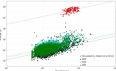
calculated by Hibert et al. (2011) for granular flows on the Dolomieu crater topography. Even though the seismic energies we obtain are smaller than those calculated during the period investigated in Hibert et al. (2011), they seem to follow the same power law (Figure 4). We compute the ratio RS∕Pfor each month and each
station (BOR, DSO, and SNE). We fit the data in a log-log scale and use a least squares regression. The fitting process and results are shown in Figure 4. We obtain the following ratio for each station, averaged over the study period:
• BOR: RS∕P= 4.12 × 10⁻⁷
• DSO: RS∕P= 1.49 × 10⁻⁶
• SNE: RS∕P= 9.69 × 10⁻⁷
To compute the RF volumes, we use the averaged seismic energy and RS∕Pratio over the three stations, with the arithmetic average RS∕Pav= 5.1 × 10⁻⁷.
For some events, we found inconsistencies between the energies computed at each station. Therefore, we selected only the consistent energies to compute the volume (see Text S2 for more details). Then, a visual
Journal of Geophysical Research: Earth Surface
10.1029/2017JF004507
Figure 4. Simulated potential energy (from ; Hibert et al., 2011) as a function of rockfall duration (in red) and observed
seismic energy as a function of seismic signal duration, along with the corresponding best fit regression lines, for the seismic stations BOR, DSO, and SNE (in black, blue, and green, respectively). We constrain the regression lines for the seismic energy to have the same slope as the one fitting the potential energy (B = 1.45). See Figure 1 for the locations of the seismic stations.
check of the seismic signals of all the events was performed, to remove potentially ambiguous events (e.g., multiple events, including volcano-tectonic ones). Because we focused on the analysis of large events in this study, we chose to check only the largest volumes (V> 3,000 m3), thus removing six (out of 63) of them (see
examples in Figures S4 and S5).
Given the complexity of the system, it is difficult to determine accurate error in the RF volume computed using seismic data. However, for a particular RF, Hibert et al. (2011) compared the volume computed using seismic data and the volume estimated from photogrammetric data. The comparison showed that the volume is overestimated by 30% using seismic data. To check the validity of the volumes we computed using seismic data, we compared them with lidar and photogrammetric data (see following section).
3.4. Volume Estimations Using Ground-Based Lidar and Photogrammetric Data 3.4.1. Acquisition and Processing of Ground-Based Lidar Data
Lidar data were acquired during a 2-day field campaign in November 2014 using a Terrestrial Laserscanner (TLS) Riegl VZ4000 with a maximum scanning distance up to 4,000 m. To provide high-resolution point data of the crater and minimize shadowing effects (Haas et al., 2016), the scanning was done from eight different scan positions around the crater rim (e.g., Figure 3b). Global positions of the scan sites were provided by externally measured reflectors (dGNSS system). After several postprocessing steps (Haas et al., 2016), including registra-tion/referencing of every single scan position (iterative closest point [ICP]-based algorithm; precision of the referencing: 0.007 to 0.013 m), thinning, and filtering (e.g., flying points in the Riscan Pro software, riegl.com), total number of points sums up to 60.106(mean point density: 55 points per square meter). Point clouds
of all single scan positions were merged and exported as ASCII files. All subsequent processing steps were performed using LIS Desktop/SAGA GIS.
3.4.2. Acquisition and Processing of Terrestrial Photographs
During two field campaigns, in 2014 (during the TLS acquisition) and 2016 (without TLS acquisition), terres-trial photographs were captured around the crater rim using two different camera systems (2014: Pentax K-x, 28 mm; 2016: Nikon D610, 28 mm). To increase the quality of the photogrammetric model, we used the scanning positions but also added some camera positions in between. Standard processing steps were per-formed with Photoscan Professional (Agisoft/Vers. 1.2.3-64bit) to produce 3-D point clouds of the terrestrial photographs:
• Pictures of every time step were aligned, and tie points (reflector targets) were automatically derived by Photoscan Professional, resulting in an initial sparse point cloud.
• To provide global coordinates, ground control points (GCPs) were set on every single picture. Given the absence of available markers inside the crater, GCPs were chosen using concise objects in the 2014 TLS point cloud. In this manner, a sum of 39 GCPs were selected, taking into account probable surface changes between 2014 and 2016, resulting in the appearance or disappearance of concise objects in the earlier or later picture.
• Using the sparse point cloud and the available GCPs, dense clouds were derived for the 2016 photographs. The total number of points was 10.106for the western part (50%) of the crater (mean point density: 10
points per square meter). After the processing procedure, the point cloud data were ASCII formatted (x,y,z, and RGB values) and exported as global coordinates. All subsequent processing steps were done using LIS Desktop/SAGA GIS in the same way as for the ground-based lidar data .
3.4.3. Quantification of Surface Changes
The ASCII files of all time steps, including TLS (2014) and Structure from Motion (2016) data, were imported to LIS Desktop/SAGA GIS (Vers. 3.0.7-64bit)/SAGA GIS (Vers. 3.1.0-64bit) by producing a SAGA point cloud. To check the orientation of both data sets, point clouds were fine-adjusted by applying the ICP adjustment (e.g., Besl & McKay, 1992) in LIS Desktop and by using only stable areas for the fine adjustment. The fine adjustment of the 2014 point cloud (slave) to the 2014 point cloud (master) was carried out successfully with a value of 0.36 m (standard deviation for all points used for the ICP). After this, point clouds were segmentized by plane fitting (SAGA LIS tool segmentation by planes) in order to produce normal vectors for these single planes (and thus for all points belonging to a certain plane). This step was necessary for the following point-to-point distance calculation using the tool distance between point clouds (e.g., Fey & Wichman, 2017). Based on this information, 3-D surface changes were obtained from the measured elevation changes (Figure 3b), and the volumes for certain areas in the western part of the crater were calculated.
3.4.4. Calculation of the Measurement Error
As each method and their combination contain measurement errors leading to uncertainties in the volume calculation, a statistical approach was used for the assessment of the error. This approach assumes that (i) the errors can be calculated using stable areas (e.g., solid rocks, Westaway et al., 2000), (ii) the errors will follow a normal distribution for these stable areas with a mean of 0 (Brasington et al., 2000), and (iii) the uncertainties are independent. The approach of Lane et al. (2003) for the estimation of the level of detection for derived dif-ferences of digital elevation models was used to calculate the error in the point-to-point distances. Therefore, the combined normal distributed error𝛿pointdistancecan be derived using the formula
𝛿pointdistance= √ 𝜎2 pointdistance+𝜎 2 pointdistance, (4)
where𝜎 = 0.32 m is the standard deviations for the point-to-point distances for the stable area for the two field campaigns, resulting in a𝛿pointdistanceof 0.45 m. The absolute value of each point-to-point distance (DP1− DP2) is then divided by𝛿pointdistanceto calculate a t score (Bennett et al., 2012):
t =|DP1− DP2| 𝛿pointdistance
. (5)
A simple t test is then conducted for each point to decide whether the change on this point is significant or not. We apply a simple probabilistic threshold (tcrit) at the 90% confidence interval (t> 1.645) to classify
surface changes as probably representing real change or measurement error (e.g., Haas et al., 2016). Thus, only point-to-point distances with real changes over 0.74 m (> tcrit) are used for the calculation of the elevation
changes (e.g., Lane et al., 2003), subtracting the single time steps, which result in positive (accumulation) or negative surface changes (erosion).
4. Results
4.1. Comparison of Seismic and Photogrammetric Method Results
We compare the volume of RFs computed using the two methods over the period from November 2014 to January 2016 (corresponding to the period of photogrammetric measurements). The RF locations provided by the two methods (Figures 3a and 3b) are consistent (both methods show the most active zone to be north northwest of the crater). The most active zone presents steep slopes and large cracks, prone to generate big RFs (OVPF database, Figure S6). This could explain the larger volumes of the RFs observed in this area. The seis-mic data (Figure 3a) show that the southwestern part of the crater is not very active, despite the presence of
Journal of Geophysical Research: Earth Surface
10.1029/2017JF004507
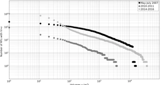
Figure 5. Comparison of the distribution of the RF volume over the periods May–July 2007 (black), 2010–2011 (dark
gray), and 2014–2016 (light gray). Theyaxis represents the number of RFs with volume greater than the corresponding volume on thexaxis. This distribution shows that the catalog of RFs is reliable for volumes greater than 100 m3. RF = rockfall.
large cracks. This observation appears to be inconsistent with the photogrammetric data (Figure 3b) that show large detached volumes but with few or no visible deposits. The discrepancy between the two data sets and the absence of deposits suggest that a different mechanism is involved here. It is inferred that subsidence is occurring on the southern edge of the crater. This assumption is consistent with the absence of seismic activ-ity in this zone, since subsidence is seismically silent. It is also consistent with the negative surface changes and the lack of corresponding deposits shown by photogrammetric data. This limited case analysis shows the value of coupling two different methods to interpret the mechanism controlling the deformation of the crater edges.
Using the photogrammetric data, we extracted the precise volume of the largest deposits in the northwestern zone of the crater, obtaining a total volume of ∼80,000 m3. We found a volume of the same order of magnitude
using the seismic method, with a total of ∼100,000 m3when adding up the volumes of RFs with V> 100 m3.
The frequency-volume distribution shown in Figure 5 follows a power law for V> 100 m3(Figure S7). For
the 2014–2016 period, the observed excess of small events is likely due to a wrong classification of small volcano-tectonic (VT) events into RFs. In the following analysis, we will consider only RFs with V>100 m3, for
which our catalog is reliable. To determine the impact of neglecting the small events, we estimate their total volume using the power law (which we believe to be more accurate that the observed count of small events). From this approach, the total volume of small RFs (V<100m3, Figure S7) is ∼8,500m3, which is a small
percent-age (8.5%) of the total volume of RFs. The lack of larger events compared to the power law prediction may be due to the existence of a maximal volume of RFs that cannot be exceeded in the crater. The volume overesti-mation when using seismic data vs. photogrammetric data may be due to errors in RF location and duration and/or to the underestimation of the slope angle. It may also be related to the use of numerical simulations of granular flows, whereas at least the first part of the RFs we observe exhibits free fall. Part of the difference between the two methods may also be due to the removal of the smallest deposits (height< 0.74 m) by the photogrammetric method. However, the 26% discrepancy observed here is similar to that found by Hibert et al. (2011) for a single RF event and supports the use of the seismic method to estimate the volume and loca-tion of RFs. In the following analysis, we will use these volumes and localoca-tions to analyze the spatiotemporal distribution of the RFs.
4.2. RF Catalog Description
Using seismic signals, we located and computed the volume of 10,477 RFs occurring between January 2014 and December 2016. The average error in the event locations is 200 m (Text S1). In Figure 6a, we do not observe the expected increase in RF number or volume just before (1 day) or during all the eruptions. On the contrary, we note a decrease in RF activity. This is the result of missing events, drowned in the noise generated by the high number of volcano-tectonic events just before the eruptions and by the volcanic tremor during the erup-tions. Some RFs are large enough to be detected (see during eruptions 2 and 3, Figure 6a). We used them in
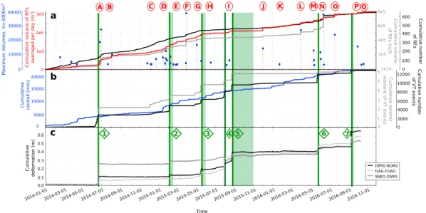
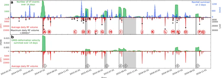
Figure 6. (a) Temporal evolution of the RFs: cumulative number (black), cumulative volume (gray), cumulative volume
averaged per day (red), and maximum volumes of individual events per day when greater than 3,000 m3(blue dots). (b)
Temporal evolution of rainfall (blue) and shallow volcano-tectonic (VT) events plotted as cumulative number (black) and cumulative seismic moment (gray). (c) Cumulative deformation of the base (light gray) and of the summit (dark gray and black) of the terminal cone. The locations of Global Navigation Satellite System stations are indicated in Figure 1. The letters denote significant increases in RF volume (steps in red and gray curves, blue dots). The green vertical lines and rectangles show the start times and durations of eruptions. RF = rockfall.
the comparison with the photogrammetric volume, but they are not considered in the following spatiotem-poral analysis because of the incompleteness of the catalog during eruptions. Outside of these periods, 122 of the located RFs have volumes greater than 1,000 m3, while 57 have volumes greater than 3,000 m3(Figure 5).
The two largest RFs have volumes close to 40,000 m3(Figure 3a).
Figure 5 presents the comparison of the volume distributions for the periods studied by Hibert et al., (2011, 2017) and for the 2014–2016 period. It shows that RF activity in 2014–2016 is lower than during the first 2-month phase of the postcollapse relaxation from May to July 2007. However, this activity is higher than during the more stable period of 2010–2011. We infer that even if more stable than during the postcollapse relaxation phase, the crater edges have been unsettled by the recovery of the eruptive activity after a 4-year break, leading to larger volumes than those at the end of the relaxation period.
4.3. Temporal Evolution of RF Activity
Figure 6 represents the cumulative number of RFs over the 2014–2016 period along with the cumulative volume of RFs (the RF number and volume per day are represented on Figure S8). We compare the total cumu-lative volume to the cumucumu-lative volume averaged per day. To compute the averaged volume per day, we divide the total volume by the number of RFs:
Vav(t) =
n(t)∑ i=1
Vi(t)
n(t) , (6)
where Vi(t) is the individual volume of each RF, and n(t) the total number of RFs occurring during day t. Plotting
the averaged volume per day highlights the importance of the larger volumes compared to the smaller ones. We observe variations on the three curves, with stronger variations of the volume than of the number of RFs. The steps indicated by letters on Figure 6 have an averaged volume per day greater than 1,500 m3and include
individual events with volumes greater than 3,000 m3(Table 1 and blue dots in Figure 6a). In the following,
we will use the term RF swarm to name these steps. The beginning and ending dates of the RF swarms are selected manually to capture the periods of volume increase.
Most of these RF swarms last 2 to 15 days, except the third one (C) that lasts 1 month. This RF swarm is actually made of three distinct episodes of volume increases separated by less than 15 days. We compare the temporal evolution of RFs with the number and seismic moment of volcano-tectonic events and with rainfall recorded at
Journal of Geophysical Research: Earth Surface
10.1029/2017JF004507
Table 1
Description of the RF Swarms Shown in Figure 6
RF Number Vmax Vav Number of events Number of events First day Duration swarm of events (m3) (m3) V>3,000 m3 V>1,000 m3 of the swarm (days)
A 115 27,700 946 5 16 2014/06/23 13.8 B 150 10,400 156 2 3 2014/07/16 18.4 C 657 7,300 77 4 6 2014/11/24 34.9 D 72 12,800 707 5 9 2015/01/13 14.5 E 243 3,700 94 3 8 2015/02/15 15.2 F 143 38,900 387 2 4 2015/03/27 6.9 G 232 17,000 118 1 3 2015/05/01 13.5 H 22 4,800 307 1 2 2015/06/15 2.7 I 94 6,400 131 2 2 2015/08/05 12.8 J 43 14,500 356 1 1 2015/11/30 2.9 K 27 3,600 189 1 1 2016/01/22 4.9 L 27 27,100 1,154 1 3 2016/03/31 2.9 M 36 13,000 899 4 5 2016/05/12 4.9 N 144 37,900 1,275 14 19 2016/06/04 11.9 O 8 23,900 3,549 1 3 2016/07/14 6.3 P 27 15,900 738 1 2 2016/09/29 6.1 Q 14 3,300 261 1 1 2016/10/12 3.6
Note. Dates are formatted as year/month/day. RF = rockfall.
a summit station on the volcano (Figure 6b). Most of the increases in RF activity seem to be related to increases in volcano-tectonic seismicity. Figure 6c presents the distance changes between pairs of GNSS stations located at the cone summit and base (Figure 1), representing the evolution of the cone deformation. It is difficult to link the deformation observed on these curves with the changes in RF volume.
To quantify the link between volcano-tectonic events, rainfall, and RF swarms, we compute the cross correla-tion between pairs of time series X and Y using the common formula:
C(X, Y) = X ∗ Y N ×𝜎X×𝜎Y,
(7) where N is the length of the time series and𝜎Xand𝜎Ytheir respective standard deviations. The cross
correla-tion between two time series is calculated several times, shifting one of the time series by 1 day. This allows us to identify the time lag that gives the best correlation. In order to obtain correlation coefficients comprised between −1 and 1, we divide them by the corresponding autocorrelations:
C(X, Y)
C(X, X)C(Y, Y). (8)
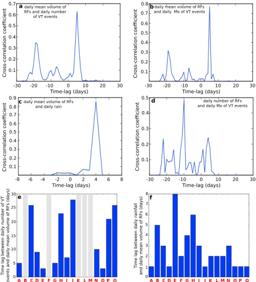
For each RF swarm (A to Q, Figure 6), we compute the cross correlation between the time series of the number of volcano-tectonic events and of the RF volume, ranging from 30 days before to 1 day after the first day of the RF swarm. We show an example of the result obtained for swarm G in Figure 7a. In the same way, we compute the cross correlations and time lags between the time series of volcano-tectonic seismic moment and the time series of the RF volume and number (swarm G, Figures 7b and 7d). We apply the same strategy to look at the cross correlation between rainfall and RF volume but using a period ranging from 8 days before to 1 day after the first day of the RF swarm (swarm G, Figure 7c).
We observe a clear correlation between the daily seismic moment of volcano-tectonic events per day and RF volume (see, e.g., swarm G in Figure 7a and Tables S1 and S2), with associated time lags ranging from 3 to 30 days (Figure 7e): 59% of the RF swarms show a correlation with the daily seismic moment of volcano-tectonic events exceeding 0.6 and 23% exceeding 0.8. The correlation between the number of volcano-tectonic events per day and RF volume is weaker: 41% of the RF swarms show a correlation with the number of volcano-tectonic events exceeding 0.6 and 12% exceeding 0.8. The correlation of seismicity with
Figure 7. Examples of cross correlation between daily mean volume of RFs and (a) daily number of volcano-tectonic
(VT) events, (b) daily seismic moment of VT events, (c) daily amount of rainfall, and (d) between daily number of RFs and daily maximum magnitude of VT events. (e) Time lags corresponding to the maximum cross-correlation coefficient between daily mean volume of RFs and daily number of VT events for each RF swarm (A–Q in Figure 6). (f ) As for (e), for cross correlation between daily mean volume of RFs and daily amount of rainfall. RF = rockfall.
the daily number of RFs is poor (Figure 7d and Tables S1 and S2). From the time lag distribution shown in Figure 7e, we use an average time lag of 14 days for the following analysis. No corresponding time lag for episodes B, F, K, L, and M means that there was no seismicity during the 30 days before these RF swarms. In the same way, we compute the cross correlation between daily rainfall and RF volume. The correlation is also good (see, e.g., swarm G in Figure 7c and Tables S1 and S2): 48% of the correlations significantly exceed 0.6 and 29% exceed 0.8, for correlation times up to 8 days. From the time lag distribution shown in Figure 7f, we use an averaged time lag of 3 days for the following analysis. This offset is in agreement with other studies (Delonca et al., 2014; Helmstetter & Garambois, 2010; Hibert, Mangeney, et al., 2017).
According to these results and to better highlight the links between the RF swarms and external forcings, we compare the daily average volume of RFs to the number of volcano-tectonic events summed over the 14 pre-vious days and to the rainfall summed over the three prepre-vious days (Figure 8a). We also compare the volume of RFs with the deformation at the summit of the volcano (Figure 8b). The increases in seismic activity often match a cone deformation episode, because both are triggered by the dike intrusion (Peltier et al., 2016; Segall et al., 2013; Staudacher et al., 2016). Since the two are linked, we chose to sum the absolute deformation veloc-ity of the summit of the volcano (SNEG-DSRG pair of stations) over the same period of 14 days as seismicveloc-ity. Note, however, that we do not capture RFs occurring during the eruptions. Consequently, the response time of RFs to seismicity or deformation may be shorter than 1 day at the time of the eruptions.
Journal of Geophysical Research: Earth Surface
10.1029/2017JF004507
Figure 8. Comparison of the temporal evolution of the external forcings with the volume of RFs averaged per day. (a, top) Number of volcano-tectonic events
summed over the prior 14 days, from dayj − 14to dayj(green), and rainfall summed over the prior 3 days, from dayj − 3to dayj(blue). (a, bottom) Averaged volume of RFs per day (red) and maximum volume per day, when it exceeds 3,000 m3(black). Note that theyaxis limits are different for the averaged and
maximum volumes. The letters denote significant increases in RF volume (Vav> 1, 500 m3andV
max> 3, 000 m3, limit indicated by the red-dotted line). The gray
vertical lines and rectangles show the start times and durations of the eruptions. (b, top) Absolute velocity of the cone deformation represented by the SNEG-DSRG baseline variations, summed over the prior 14 days. (b, bottom) Same as (a). RF = rockfall; GNSS = Global Navigation Satellite System; VT = volcano-tectonic.
We observe clearly in Figure 8a that all the bursts of volcano-tectonic events are related to RF swarms in the following 14 days (swarms A, C, D, G, I, N, O, and P). In the same way, most of the cone deformation episodes are also followed or concomitant with a RF swarm (Figure 8b). Most of the RF swarms are also preceded by rainfall (48% of the RF swarms show a significant correlation with rainfall during the eight previous days). However, large rainfalls does not necessarily trigger a RF swarm (e.g., the rain episode of February 2016 in Figure 8a). 4.4. Spatiotemporal Evolution of RF Activity
Figures 9, 10, and 11 show the spatiotemporal evolution of RFs during swarms A to Q. The first RF swarm occurs after the first eruption following the 4-year break. The slopes of the crater are homogeneously desta-bilized during swarm A, with small and large RFs. This first swarm is remarkable owing to the high number of volumes greater than 1,000 m3(16, Table 1 and Figure 9a). The RF distribution is still homogeneous during
swarms B and C. During swarm C, the activity begins to concentrate in the northwestern part of the crater. The most active north northwestern zone shows more small RFs, smaller than 1,000 m3. Most of the small
RFs will indeed occur in this zone over the whole period. Note that this zone corresponds to the steepest and most fractured slopes of the crater. Five months after eruption 1, swarms C and D activate this area with large volumes, greater than 3,000 m3(Figures 9c and 9d). This zone is very active until May 2015 (Figures 9c,
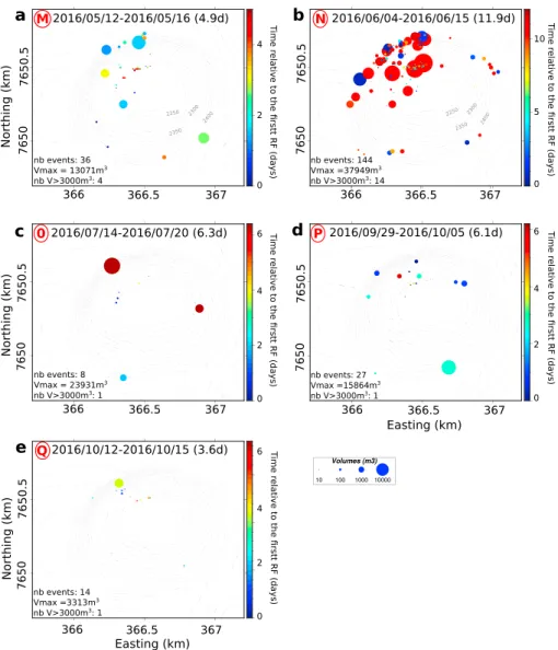
9d, 9f, and 10a), showing a long-term relaxation of about 6 months. Then, after swarm G and during 1 year, this area shows very little activity, with only small RFs, even during the different swarms (Figures 10b–10f ). In May 2016, events larger than 10,000 m3reactivate this northwestern zone, before swarm N, when the second
largest volume (37,900 m3) of the studied period occurs (Figures 11a and 11b). Then the RF activity seems to
quiet down again until the end of 2016 (Figures 11c–11e). From November 2014, most of the large events that are preceded by a seismic crisis (C, D, E, G, N, O, and P) are located in the active northwestern part of the crater. On the other hand, the largest volumes of swarms not directly explained by seismicity (B, F, H, J, K, and L) occur on the other slopes. This is the case of the largest event of the period (V = 38,800 m3, Figure 9f ).
In order to look at the impact of eruptive activity on the RF distribution, we plot the spatiotemporal evolution of the RFs between the eruptions (Figures 12 and 13). The first observation we can make is that RFs are larger after the first eruption than before (Figures 12a and 12b). In both cases (before and after eruption 1), they are homogeneously distributed around the crater even if they are slightly more concentrated in the north northwestern zone. After the second eruption, they tend to concentrate in the north northwestern part, with smaller volumes. The volumes increase again before the sixth eruption, in the north northwestern active area, but also on the side of the crater closest to the eruption (Figure 13b). This eruption is followed by one of the largest RFs of the 2014–2016 period. This RF is located in the most active zone of the crater and closer to the seventh eruption location.
Figure 9. (a–f ) Spatial distribution of the RFs making up the A–F swarms shown in Figure 6. For each swarm, the time
span corresponds to its duration. Each round dot represents a RF, and its radius is proportional to the RF volume. The colors of the round dots indicate the time from the first RF of the swarm. RF = rockfall.
Looking at the spatial distribution of the RFs during the days preceding all the eruptions, the unstable north northwestern zone is almost always destabilized, but we also note a tendency of the largest RFs to concentrate on the crater edge closest to the next eruption location, a few days before. This is observed for summital eruptions (numbers 1 and 2 in Figure 12) and for most of the distal ones (numbers 3, 4, 6, and 7 in Figures 12 and 13). Eruptions 2, 4, and 7 occur on the northwestern side of the crater, close to the most destabilized zone. It is thus difficult to link them to RF activity occurring in this area. As for eruptions 1, 3, and 6, they occur on the opposite side, much less active in terms of RFs (Figures 3a, 9, 10, and 11). However, events of average to large volumes occur in this zone a few days before these eruptions (Figures 12, 13, and 14). Furthermore, a more detailed investigation of what is happening during the four RF swarms preceding eruptions (swarms D, G, I, and M, occurring during the 20 days preceding eruptions 2, 3, 5, and 6, respectively) shows that the largest RFs tend to migrate toward the next eruption location (Figure 14).
5. Discussion
5.1. Evolution of the RF Activity Compared to the Postcollapse Period
The period we analyze is far enough from the 2007 crater floor collapse to be less affected by the postcol-lapse relaxation of the crater slopes. Furthermore, it corresponds to the renewal of eruptive activity of the volcano after a break of 41 months. This resurgence in volcanic activity was accompanied by a high activity
Journal of Geophysical Research: Earth Surface
10.1029/2017JF004507
Figure 10. Same caption as Figure 9 for rockfall swarms G–L.
of volcano-tectonic events: more than 2,000 seismic events occurred during the 2 weeks preceding the June 2014 eruption (Lengliné et al., 2016). The RF activity during the 2014–2016 period is higher than that at the end of the relaxation period, from 2010 to 2011 (Figure 5). We infer that the increase in the RF activity com-pared to the 2010–2011 period is the signature of crater slope destabilization due to the renewal of volcanic activity, accompanied by the resumption of volcano-tectonic seismicity and deformation. The RFs constitut-ing the first RF swarm (A) of the period are located homogeneously around the crater (Figure 9a). They are subsequently preferably located in the most active zone, northwest of the crater (Figure 3). However, before most of the eruptions (85%), the largest RFs tend to migrate toward the eruption location in the days leading up to the eruption (Figures 12 and 13). This corroborates Hibert, Mangeney, et al.’s (2017) observations on RF migration before eruptions. Another interesting observation over the 2014–2016 period is that eruption num-ber 6, like eruption numnum-ber 1, seems to reactivate slope instability at different places in the crater (Figures 13b and 13c). One common feature of eruptions 1 and 6 is that they both occur after a quiet period of more than 1 year. This may explain the similarities observed in the RF response to these eruptions. During the period of quiescence, the RFs are subjected to a long-term forcing caused by gravity and rainfall episodes. We infer that this long forcing initiates the destabilization of the slopes, while the sudden high seismicity associated with the renewal of volcanic activity triggers the simultaneous fall of all the unsettled slopes.
The RS∕Pratio we calculate for the 2014–2016 period is smaller than the one obtained by Hibert et al. (2011) for
Figure 11. Same caption as Figure 9 for rockfall swarms M–Q.
seismic efficiency RS∕Pare a key issue. Different values have been found in different environments: RS∕Pvalues
ranging from 10−5to 10−3have been found by Hibert et al. (2011) for the Piton de la Fournaise volcano over the
2007–2011 period and by Deparis et al. (2008) for RFs in the French Alps. On the other hand, smaller RS∕Pvalues
ranging from 10−6to 10−5have been found by Levy et al. (2015) for granular flows in Montserrat valleys and by
Berrocal et al. (1978) for a landslide in Peru. Free-fall laboratory experiments of beads and grains have shown that the seismic energy dissipated during an impact depends on the grain size and velocity, on the nature of the receiving plate, and on the slope angle (Farin et al., 2016, 2018), as confirmed by field measurements (Hibert, Malet, et al., 2017). Furthermore, Bachelet et al., (2016, 2018) have shown that the presence of an erodible bed can decrease the seismic energy transmitted to the ground for free-fall grains, in agreement with field observations of rock impact (Farin et al., 2015). The reason is that part of the acoustic energy is dissipated in the erodible bed by inelastic collision and agitation of grains. We can thus possibly explain the smaller ratio (i.e., seismic energies) obtained here compared to those of Hibert et al. (2011) by the smaller size of the 2014–2016 RFs and by the presence of an erodible bed due to the accumulation of RF deposits after the crater collapse.
5.2. Link Between RFs and External Forcings
Looking at the temporal evolution of the RFs (Figure 6), we observe small changes in their rate of occurrence, related to eruption times and rainfall amounts. We notice an interaction between seismic events and RFs, with a response time of several days (Figure 8a). This vibration-induced destabilization of crater slopes could be compared to the delayed dynamic triggering of earthquakes, where the impingement of remote or local
seis-Journal of Geophysical Research: Earth Surface
10.1029/2017JF004507
Figure 12. Spatiotemporal evolution of RFs during intereruption periods (eruptions 1 to 4). The pink diamond denotes
the upcoming eruption. Each round dot represents a RF, and its radius is proportional to the RF volume. The colors of the round dots denote the time to the upcoming eruption. The gray and black arrows represent the horizontal displacements at the summit during the intereruption period and the first day of the eruption, respectively. The red letters indicate the RF swarm present in each plotted period. (a) Eruption 1: 20 and 21 June 2014, (b) Eruption 2: 4–15 February 2015, (c) Eruption 3: 17–30 May 2015, and (d) Eruption 4: 30 July to 2 August 2015. RF = rockfall.
mic waves on a granular fault gouge drives it to failure or slip (Gomberg & Johnson, 2005; Hill & Prejean, 2006). Several laboratory investigations on sliding of a frictional interface (Bureau et al., 2001; Capozza et al., 2009; Léopoldès et al., 2013) and dynamics of a granular medium (Johnson & Jia, 2005; Johnson et al., 2008; Lastakowski et al., 2015) subjected to external vibrations provide clues to the role of seismic waves in fault instability. Jia et al. (2011) and Léopoldès et al. (2013) have shown that ultrasounds can lubricate the grain contact bonding via vibration-induced growth of microslips or cracks, decreasing the elastic modulus and the static threshold of granular media and consequently triggering the failure. Similar to the destabilization pro-cess studied here, Jaeger et al. (1989) have also found that the angle of repose of a vibrated sandpile relaxes quasi-logarithmically in the course of time. They showed that such relaxation phenomena could be explained by an activation process in which mechanical vibration could play a role of effective temperature Teffin dense
Figure 13. Same as Figure 12 for eruptions 5 to 7. (a) Eruption 5: 24 August to 31 October 2015, (b) Eruption 6: 26 and
27 May 2016, and (c) Eruption 7: 11–18 September 2016.
granular media (Liu & Nagel, 1998), being proportional to the vibration energy (Léopoldès et al., 2013). This may describe the transition from jammed solid to flowing liquid states.
Such an activation mechanism is reminiscent of thermal activation involved in crack nucleation (Das & Scholz, 1981) or the rate-and-state-dependent friction process (Baumberger & Caroli, 2006; Di Toro et al., 2011). The latter has been invoked to explain earthquake nucleation (Dieterich, 1979; Rice & Ruina, 1983; Scholz, 2002) where the characteristic time to failure may be estimated from the critical slip distance (Campillo & Ionescu, 1997; Dieterich, 1992) and the slow rupture velocity, ranging from a few microseconds to a few minutes or a few days for different systems (Latour et al., 2013). A nucleation process may thus explain the observed time delay of a few days for RF triggering, where the number or repetitions of seismic events plays a more important role than their maximum magnitude, possibly due to the effect of vibration energy (i.e., Teff) rather than a pulsed stress, in the phenomena leading to rupture.
We estimate the dynamic strain required in laboratory experiments and field observations to trigger the instability. In the case of model granular media, an ultrasound of f ∼ 10–100 kHz induces a displacement of u ∼ 1–10 nm. With a wave velocity of c ∼ 100–500 m/s (Jia et al., 2011; Johnson & Jia, 2005), the dynamic strain𝜖d = 2𝜋u∕𝜆 is of the order of ∼10−6(with wavelength𝜆 = c∕f). At the Piton de la Fournaise volcano,
the displacement at the summit of the volcano triggered by the S wave of volcano-tectonic events of M ∼ 3 (maximum magnitude of these events) is of the order of 10−7m for a vibration velocity of around 10−5m/s at a
Journal of Geophysical Research: Earth Surface
10.1029/2017JF004507
Figure 14. Zoom on the four RF swarms (D, G, I, and M) preceding eruptions
number 2, 3, 5, and 6. Each round dot represents a RF, and its radius is proportional to the RF volume. The colors of the periphery of the round dots correspond to the related eruption (colored diamonds). The intensity of the round dot colors shows the time to the eruption. The letters in the colored bars correspond to the RF swarms shown in Figure 8a. (2) 4–15 February 2015, (3) 17–30 May 2015, (5) 24 August to 31 October 2015, and (6) 26 and 27 May 2016. RF = rockfall.
frequency of about 10 Hz. The S wave velocity in a highly fractured basaltic media is about 500 m/s, producing a dynamic strain on the order of 10−8,
which is smaller than the values found in the above laboratoryexperi-ments and in some cases of dynamic triggering of earthquakes (Gomberg & Johnson, 2005). The extrapolation of laboratory experiments to natu-ral conditions needs further investigation. This is especially the case for the Piton de la Fournaise volcano, given that the effect of the cone defor-mation and rainfall must be taken into account in addition to seismic activity.
Even if we assume that the effect of the postcollapse relaxation of the crater slopes is no longer dominant, it is still difficult to discriminate between the influences of the different factors on RF activity. Indeed, there are intricate relations between volcanic seismicity, cone deformation, rain-fall, and RFs. First, volcano-tectonic seismicity and deformation are linked and often simultaneous. They are both triggered by the pressurization at depth of the volcanic system and by the migration of the magma. Sec-ond, Piton de la Fournaise is exposed to a tropical climate with some of the highest rainfall intensities in the world (with an average of 7,000 mm/year). Because of the high activity of the volcano, rain is often coincident with seismicity and/or cone deformation. However, from the observations in Figure 8, volcano-tectonic events seem to play a predominant role. Indeed, all the increases in seismic activity are followed by a RF swarm, even if there is little deformation and little rainfall (e.g., the C swarm in Figure 8, with a maximum volume of 17,000 m3, was preceded by relatively low rainfall,
129 mm over the 10 previous days). Nor is it obvious that rainfall is suffi-cient to trigger large RFs (V> 15,000 m3) in the Piton de la Fournaise crater
(Figure 8a). In this context, it is thus difficult to determine the exact influ-ence of rainfall on the increases in RF volume. From our observations, it seems that even small seismicity (M< 3) observed at the Piton de la Four-naise volcano can generate higher RF activity. However, in this volcanic context, it is likely that the combined action of seismicity and rain leads to the increase of RF activity we observe: Subcritical crack growth processes may be very efficient, triggered by seismicity (as described in the previous paragraph) and enhanced by infiltration of meteoric water in cracks interacting with volcanic gases (Atkinson & Meredith, 1987; Kilburn & Voight, 1998).
During our study period, seven RF swarms out of 17 (B, F, H, J, K, L, and M in Figure 8) are not directly explained by seismic activity, deformation, or rainfall. The largest volumes of swarm B occur on the southern and east-ern slopes of the crater (Figure 9b), destabilized about 10 days before, during RF episode A. We infer that this corresponds to the relaxation of this area after the activity triggered 1 month earlier by the first eruptive activ-ity since the 41-month break. Note that a small rainfall event occurred before swarm B. As for swarms F, H, J, K, and L, they consist of a few large events (>3,000 m3) located outside of the northwestern zone and some
small ones (<1,000 m3) in the northwestern zone. They are not preceded by seismicity nor significant
defor-mation during the previous days. Neither are any of these swarms, except K, preceded by significant rainfall. The observation of these five RF swarms (F, H, J, K, and L) suggests that the destabilization of large volumes outside of the steepest slopes seems to be a long-term process. We infer that the renewal of volcano-tectonic activity destabilized the whole crater on the short and long term with a delay of a few days for the steepest slopes until the end of their relaxation and several months for the more stable slopes. To confirm that the large volumes of swarms F, H, J, K, and L are linked to the renewal of volcano-tectonic activity, another study should be carried during a period with no significant seismicity. We highlight here a different behavior of the RFs, depending on the steepness of the slopes. The steepest slopes (NW of the crater) are prone to generate many RFs of various sizes and respond quickly (a few days) to seismic activity. On the other hand, the smoothest slopes exhibit fewer RFs and mainly large ones. They generally respond to the combined action of seismicity and rain with a delay of more than 1 month.
Finally, swarm M occurs mainly in the most active zone of the crater and consists of a few large events (>3,000 m3) along with small events (<200 m3, Figure 11a). It occurs during a small rainfall event, without
seis-micity nor significant deformation during the previous days (Figure 8). It is difficult to conclude that this limited rainfall event could be sufficient to trigger such a change in RF volumes. Another possibility could be that the destabilization of the area is a long-term process. Indeed, there was no large RF on the northwestern slope for 12 months (Figures 10b–10f, 12d, and 13a) after the relaxation of RF activity due to the renewed eruptive activity. However, there were seismic activity, deformation, and rainfall during this period that, together with the force of gravity, could have progressively destabilized the area. Subsequently, a small amount of rain and deformation could be sufficient to trigger large RFs. This hypothesis is consistent with the fact that swarm M marks the beginning of a second destabilization episode, lasting 2 months, with 14 RFs of volumes greater than 3,000 m3.
The vertical slopes of the Dolomieu crater form a system at its limit of stability in relation to the permanent exposure to gravitation forces. For this reason, a small disturbance can be sufficient to unsettle these slopes. Thus, the initiation of a crack or small changes in material cohesion or pressure resulting from seismic activ-ity, deformation, or rainfall may trigger larger RFs, after a time delay of several days in the case of the Piton de la Fournaise volcano. Numerical simulations and laboratory experiments taking into account the long-term effect of gravity could provide more information on what controls the time delays of subsequent large RFs. To better understand and discriminate between the influences of seismicity and rainfall on RF volume, fur-ther study should be carried out over the transition period, from 2010 to 2014, during which fur-there were no eruptions and low seismic activity.
6. Conclusions
The Piton de la Fournaise volcano represents a unique site to study the response of unstable slopes to dif-ferent forcings. The existence of a large seismic data set along with photogrammetric data allowed us to compare and show good agreement between the location and volume of the RFs estimated using these two types of data (Figure 3). Coupling these two different data sets also sheds light on the mechanisms control-ling the deformation of the crater edges. Our study shows the complexity of the Piton de la Fournaise system, with intricate interactions between RFs, eruptive activity (deformation and seismicity), and rainfall. Despite this complexity, we were able to extract information on response times of RFs to the different external forc-ings. Hibert, Mangeney, et al. (2017) pointed out a two-step relaxation phase after the 2007 crater collapse: 2 months of strong RF activity, followed by a decrease of the rate of occurrence and volume of RFs, until reach-ing a constant frequency 3 years later. Our study throws some light on smaller-scale response times between external forcings and RF activity. Seismicity, deformation, and rainfall can trigger an increase in RF volume that can last for 10 days to 1 month. These RF swarms occur after certain delays: 3 days for rain and 3 to 20 days for seismicity and deformation. A longer-term response of RFs to seismic activity and deformation is observed on the sides of the crater presenting lower slopes. By comparing our observations with laboratory experiments performed on granular materials (Jia et al., 2011; Léopoldès et al., 2013), we suggest that seismic activity could lead to the collapse of large volumes after a delay of one to several days: the repetition of vibration decreases the yield stress via crack growth or slip propagation in highly fractured or granular materials. This subcritical crack growth process may be enhanced by fluid-crack interaction due to rainfall. We also extract information on the spatial distribution of RFs in response to a localized forcing such as eruptions. Like Hibert, Mangeney, et al. (2017), we highlight a tendency of RF activity to migrate, following the locations of the eruptions.
References
Abellan, A., Vilaplana, J. M., Calvet, J., Garcia-Selles, D., & Asensio, E. (2011). Rockfall monitoring by Terrestrial Laser Scanning case study of the basaltic rock face at Castellfollit de la Roca (Catalonia, Spain). Natural Hazards and Earth System Sciences, 11, 829–841.
Aki, K., & Richards, P. G. (1980). Quantative seismology: Theory and methods (2nd ed., 645 pp.). Sausalito, CA: University Science Books. Ambraseys, N., & Bilham, R. (2012). The Sarez-Pamir earthquake and landslide of 18 February 1911. Seismological Research Letters, 83(2),
294–314.
Atkinson, B. K., & Meredith, P. G. (1987). The theory of subcritical crack growth with applications to minerals and rocks in fracture mechanics of
rock Edited by B. K. Atkinson. London: Academic. 11–166.
Bachelet, V., Mangeney, A., de Rosny, J., & Toussaint, R. (2016). Effect of the surface roughness on the seismic signal generated by a single rock
impact: Insight from laboratory experiments. Vienna Austria: EGU abstract.
Bachelet, V., Mangeney, A, de Rosny, J., Toussaint, R., & Farin, M. (2018). Elastic wave generated by granular impact on rough and erodible surfaces. Journal of Applied Physics, 123(4), 44901.
Baillard, C., Crawford, W. C., Ballu, V., Hibert, C., & Mangeney, A. (2014). An automatic kurtosis-based P- and S-phase picker designed for local seismic networks. Bulletin of the Seismological Society of America, 104(1), 394409.
Baumberger, T., & Caroli, C. (2006). Solid friction from stickslip down to pinning and aging. Advance Physics, 55, 2794348.
Bennett, G. L., Molnar, P., Eisenbeiss, H., & McArdell, B. W. (2012). Erosiononal power in the Swiss Alps: Characterization of slope failure in the Illgraben. Earth Surface Processes and Landforms, 37(9), 1627–1640.
Acknowledgments
The permanent GNSS and seismic data used in this paper were collected by Observatoire Volcanologique du Piton de la Fournaise/Institut de Physique du Globe de Paris (OVPF/IPGP). GNSS and seismic data are accessible at the Volobsis website:
http://volobsis.ipgp.fr/. This work was funded by ERC Slidequakes. We want to thank Pr Di Toro and two anonymous reviewers for their thoroughgoing reviews that helped us to greatly improve our manuscript, as well as the Editor and Associate Editor for their helpful comments.