Carbon-based models of individual tree growth: A critical appraisal

HAL Id: hal-00884173

https://hal.archives-ouvertes.fr/hal-00884173

HAL is a multi-disciplinary open access archive for the deposit and dissemination of sci-entific research documents, whether they are pub-lished or not. The documents may come from teaching and research institutions in France or abroad, or from public or private research centers.

L’archive ouverte pluridisciplinaire HAL, est destinée au dépôt et à la diffusion de documents scientifiques de niveau recherche, publiés ou non, émanant des établissements d’enseignement et de recherche français ou étrangers, des laboratoires publics ou privés.

Xavier Le Roux, André Lacointe, Abraham Escobar-Gutiérrez, Séverine Le

Dizès

To cite this version:

Xavier Le Roux, André Lacointe, Abraham Escobar-Gutiérrez, Séverine Le Dizès. Carbon-based models of individual tree growth: A critical appraisal. Annals of Forest Science, Springer Nature (since 2011)/EDP Science (until 2010), 2001, 58 (5), pp.469-506. �10.1051/forest:2001140�. �hal-00884173�

Review

Carbon-based models of individual tree growth:

A critical appraisal

Xavier Le Roux

_{, André Lacointe}

_{, Abraham Escobar-Gutiérrez}

and Séverine Le Dizès

a_{U.M.R. PIAF (INRA-Université Blaise Pascal), Site de Crouel, 234 av. du Brezet,}

63039 Clermont-Ferrand Cedex 02, France

b_{Forestry Commission, Northern Research Station, Roslin, Edinburgh, Midlothian EH25 9SY, UK} c_{Present address: Horticulture Research International, Wellesbourne, Warwick CV35 9EF, UK}

(Received 7 September 2000; accepted 1st February 2001)

Abstract – Twenty-seven individual tree growth models are reviewed. The models take into account the same main physiological pro-cesses involved in carbon metabolism (photosynthate production, respiration, reserve dynamics, allocation of assimilates and growth) and share common rationales that are discussed. It is shown that the spatial resolution and representation of tree architecture used mainly depend on model objectives. Beyond common rationales, the models reviewed exhibit very different treatments of each process involved in carbon metabolism. The treatments of all these processes are presented and discussed in terms of formulation simplicity, ability to ac-count for response to environment, and explanatory or predictive capacities. Representation of photosynthetic carbon gain ranges from merely empirical relationships that provide annual photosynthate production, to mechanistic models of instantaneous leaf photosynthe-sis that explicitly account for the effects of the major environmental variables. Respiration is often described empirically as the sum of two functional components (maintenance and growth). Maintenance demand is described by using temperature-dependent coefficients, while growth efficiency is described by using temperature-independent conversion coefficients. Carbohydrate reserve pools are general-ly represented as black boxes and their dynamics is raregeneral-ly addressed. Storage and reserve mobilisation are often treated as passive pheno-mena, and reserve pools are assumed to behave like buffers that absorb the residual, excessive carbohydrate on a daily or seasonal basis. Various approaches to modelling carbon allocation have been applied, such as the use of empirical partitioning coefficients, balanced growth considerations and optimality principles, resistance mass-flow models, or the source-sink approach. The outputs of carbon-based models of individual tree growth are reviewed, and their implications for forestry and ecology are discussed. Three critical issues for these models to date are identified: (i) the representation of carbon allocation and of the effects of architecture on tree growth is Achilles’ heel of most of tree growth models; (ii) reserve dynamics is always poorly accounted for; (iii) the representation of below ground proces-ses and tree nutrient economy is lacking in most of the models reviewed. Addressing these critical issues could greatly enhance the relia-bility and predictive capacity of individual tree growth models in the near future.

carbon allocation / photosynthesis / reserve dynamics / respiration / tree carbon balance

* Correspondence and reprints

Tel. 33 4 72 43 13 79; Fax. 33 4 72 43 12 23; e-mail: leroux@biomserv.univ-lyon1.fr

Present address: Laboratoire d’écologie microbienne des sols, UMR 5557 CNRS-Université Lyon I, bât 741, 43 bd du 11 novembre 1918, 69622 Villeurbanne, France.

Résumé – Les modèles de croissance d’individus arbres basés sur le fonctionnement carboné : une évaluation critique. Vingt-sept modèles simulant la croissance d’arbres à l’échelle individuelle sont évalués. Ces modèles prennent en compte les principaux processus impliqués dans le métabolisme carboné (assimilation photosynthétique, respiration, dynamique des réserves, allocation des assimilats et croissance). Les concepts communs à tous ces modèles sont discutés. Il est montré que l’échelle d’espace et la représentation de l’archi-tecture utilisées dépendent principalement des objectifs du modèle. Au-delà de concepts communs, les modèles évalués utilisent des re-présentations très différentes pour chacun des processus impliqués dans le métabolisme carboné. Les différentes rere-présentations de ces processus sont présentées et discutées en termes de simplicité de formulation, de capacité à prendre en compte la réponse aux variables environnementales, et de capacités prédictives. La représentation des gains de carbone va de relations purement empirique calculant la production annuelle de photosynthétats jusqu’à des modèles de photosynthèse foliaire à bases mécanistes prenant explicitement en compte les effets des principales variables environnementales. La respiration est souvent décrite de façon empirique comme la somme de deux composantes (maintenance et croissance). La demande de maintenance est calculée à partir de coefficients dépendant de la tem-pérature, alors que l’efficience de croissance est calculée à partir de coefficients de conversion indépendant de la température. Les réser-ves carbonées sont généralement représentées comme des boîtes noires, et leur dynamique est rarement prise en compte. La mise en réserve et l’utilisation des réserves sont souvent traitées comme des processus passifs, les réserves servant souvent de compartiment tam-pon absorbant les assimilats produits en excès sur une base journalière ou saisonnière. De nombreuses approches ont été utilisées pour modéliser l’allocation de carbone, telles que l’utilisation de coefficients d’allocation empiriques, l’application des principes de l’équi-libre fonctionnel et d’optimisation, l’utilisation de schémas flux-résistance, ou des approches sources-puits. Les sorties des modèles si-mulant le bilan carboné et la croissance de plantes ligneuses à l’échelle individuelle sont présentées, et leurs implications en foresterie et en écologie sont discutées. Trois points particulièrement critiques actuellement pour ces modèles sont identifiés : (i) la représentation de l’allocation du carbone et des effets de l’architecture sur la croissance de l’arbre est le talon d’Achille de la majorité de ces modèles ; (ii) la dynamique des réserves est toujours faiblement représentée ; (iii) la représentation du fonctionnement racinaire et de la gestion des nu-triments dans l’arbre est absente dans presque tous les modèles évalués. Une meilleure prise en compte de ces points critiques devrait for-tement améliorer la fiabilité et les capacités prédictives des modèles de croissance d’arbres à l’échelle individuelle dans le futur. allocation du carbone / bilan carboné de l’arbre / dynamique des réserves / photosynthèse / respiration

1. INTRODUCTION

Mathematical modelling has been used as a powerful tool in many fields of scientific activity. A model is usu-ally a simplification of the real system, and is in some re-spect more convenient to work with [127]. In particular, simulation models offer a convenient way to represent current scientific understanding and theory in complex biological systems such as trees. During the last two de-cades, emphasis on tree growth modelling has changed from merely statistical (i.e. descriptive and predictive under particular conditions) models, to mechanistic (i.e. explanatory) process-based models [45]. The latter are often based on a detailed description of physiological processes. Thus, they are complex and mostly restricted to research and educational applications, while statistical models are usually devoted to management applications [63, 83, 128]. Neither empirical nor mechanistic formu-lations are a priori preferable. The kind of formulation should be chosen according to the modeller’s objectives. Furthermore, purely mechanistic tree growth models are scarce. Generally, depending on the purpose of the model and the level of understanding of the processes involved, model designers concentrate more or less on a few partic-ular processes, and mix both process-based and statisti-cal formulations.

For these reasons, there are many tree growth models of different types, and the ongoing development of new models without a clear knowledge of the existing ones may be a waste of research resources [15]. Thus, it is highly useful to assess the range of models currently ex-isting, and identify key strategies of model structure and development. A critical evaluation of carbon-based tree growth models has already been published by Bassow et al. [7]. However, the authors only reviewed a few sim-ulation models, and focused exclusively on their suitabil-ity for assessing the effects of pollution on growth of coniferous trees. Furthermore, the analysis was concen-trated on a particular model of forest growth in stands [80]. Recently, Ceulemans [15] reviewed ten models of tree and stand growth. However, most of the models re-viewed did not treat important processes involved in tree growth (e.g. carbon allocation) and were designed to simulate only carbon and/or water exchanges between tree stands and the atmosphere.

The present paper is a critical analysis of twenty-seven carbon-based growth models of individual woody plants, and of their ability to predict plant response to various environmental conditions. Reference is also made to a generic model of plant growth that could pro-vide a useful framework for individual tree growth mod-els [128]. By contrast, modmod-els that are beyond the scope of this review are: (i) models of radiation and gas ex-change between trees and the atmosphere that do not

focus on carbon processes driving tree growth (e.g. MAESTRO [135]; CANLIP [17]; PGEN [35]; RATP [118]), (ii) models of forest growth in stands that are not explicitly based on individual tree growth (e.g. [12, 27, 64]; see also the review by Tiktak and van Grinsven [131]), (iii) models that were used to simulate shoot growth without integrating carbon balance and growth at the whole-tree scale [11, 33, 49] and (iv) individual-based forest models or morphological tree growth mod-els that do not explicitly represent the major processes in-volved in tree growth and carbon balance (e.g. SORTIE [89]; FRACPO [18]; [57, 101]). It should be mentioned that our paper does not aim at providing an extensive re-view of all the models of individual tree growth pub-lished to date, but rather a comprehensive and critical view (from a sample of models) of what has been done and remains to be done in this research area.

The twenty-seven carbon-based models of individual tree growth that were reviewed are presented in table I. Typically, these models operate at a time step ranging from one hour to one year, and either deal with whole-tree processes (e.g. whole whole-tree photosynthesis) or sum processes that occur at spatial scales smaller than a single tree (e.g. shoot or leaf photosynthesis). The individual tree is often divided into a number of compartments (i.e. organ classes) and/or individual organs. The objectives of the models range from simulating tree growth and wood production of a single tree representative of a stand, to simulating fruit production, tree architecture dynamics, or individual tree function within a vegetation dynamics framework (table I). In a first section, we pres-ent the common framework and rationales shared by all the models. The dependence of the time and space levels used and representation of tree architecture employed on model objectives is analysed. The way all the models rep-resent, to a certain extent, the relationships between tree structure and function is also studied. In a second section, the different approches used to model each process in-volved in tree carbon metabolism (photosynthate pro-duction, respiration, carbon allocation and growth, storage and reserve mobilisation) are reviewed. We dis-cuss these different treatments in terms of formulation simplicity, ability to account for response to environ-mental variables, and explanatory or predictive capaci-ties. For each process, the correlation between the formulation chosen and the time and space levels used is studied. In a third section, the outputs of carbon-based models of individual tree growth are reviewed, and their ecological implications are discussed. In the last section, major critical issues for individual tree growth models to date are identified.

2. GENERAL FRAMEWORK OF CARBON-BASED MODELS OF INDIVIDUAL TREE GROWTH

2.1. Processes accounted for and common rationales used

Whatever their objectives and levels of application, the carbon-based models of individual tree growth re-viewed generally encompass different sub-models, each describing one of the main carbon processes, i.e. photosynthate production, respiration, reserve dynamics and allocation of assimilates within the tree (figure 1). In-deed, the processes driving the carbon dynamics and growth remain fundamentally identical between differ-ent tree species, and only differ in their species- and site-specific parameters [62]. Thus, although many models have been developed for one or several particular species (table I), most of them can be applied to a range of tree species when suitably parameterised.

To a certain extent, all these models can be viewed as mechanistic models of tree growth that formulate rates of change in several state variables of the tree system by us-ing differential (or difference) equations, in contrast to purely empirical models that translate empirical observa-tions into suitable mathematical relaobserva-tionships (such as yield tables for instance). Because all these models try to correctly capture the relevant processes involved in tree growth, they thus all exhibit potential to be applied under a range of novel environmental conditions [12]. To a cer-tain extent, all the models reviewed use this potential for assessing the effect of changes in environmental condi-tions (e.g. changes in water or nutrient availability, in-crease in CO2 level, temperature, or pollutant load), predicting the impact of changes in disturbance regime (herbivory intensity or pruning practice), or matching clones to sites and predicting their potential growth, among other issues (table I). However, such predictive potential outside the range of data used for model devel-opment is more or less important according to the formu-lations used for the key carbon processes (see Sect. 3).

At least, even models using different formulations for a given process can use common rationales to represent this process. For instance, tree models represent carbon allocation by very different approaches, ranging from “morphological” modules predicting the result of translocation without any reference to the underlying mechanisms (e.g. functional balance approach) to simplified representations of the basic translocation mechanisms (namely transport resistance modules)

Table I. The 27 carbon-based models of individual tree growth reviewed. The generic model of forest growth proposed by Thornley [128] is included because it provides a useful framework for individual tree growth models.

Model Main references Major objectives Tree species Single tree

representation

Time step

– Promnitz

(1975)

Simulating tree growth

response to changes in nutrient and moisture regimes (greenhouse conditions)

Populus sp. 4 organ classes Hour/Day

PT Ågren and

Axelsson (1980)

Simulating the growth of a 15-year old Scots pine

throughout one year

Pinus sylvestris

8 organ classes Day

– Valentine

(1985)

Modelling growth rates of tree basal area and height

– 3 organ classes (active and disused pipes between foliage and roots)

Year

– Mäkelä and

Hari (1986)

Individual tree-based stand growth simulation

Pinus sylvestris

4 organ classes Year

FORSKA Prentice et al. (1990; 1993)

Simulation of natural forest dynamics in a current or changing environment

– 2 organ classes (only

aboveground)

2 years

ECOPHYS Rauscher et al. (1990); Host et al. (1990)

Simulation of first-year poplar clones under near-optimum conditions

Populus sp. Individual leaves and internodes + total root system

Hour/Day

– Thornley

(1991)

Forest growth model – 5 organ classes×

4 tissues/bioch. pools Day – Webb (1991) Predicting the growth of tree

seedlings under high CO2

levels

Pseudotsuga menziesii

5 organ classes 5 min to 1 h

VIMO Wermelinger

et al. (1991)

C and N assimilation and allocation, and impact of herbivory

Vitis vinifera 4 organ classes× n age subclasses× 2 bioch. pools

Day

TREGRO Weinstein et al. (1992)

Simulating tree physiological responses to multiple environmental stresses Picea rubens Picea ponderosa 12 organ classes× 3 bioch. pools Hour/Day WHORL Sorrensen-Co-thern et al. (1993)

3D development of tree crown structure

Abies amabilis Parts of the crown, i.e. whorl sectors (only aboveground)

Year

– West (1993) Predicting annual above-ground

tree growth in even-aged forest monoculture

Eucalyptus regnans

3 organ classes (only aboveground)

Year

PEACH Grossman and

DeJong (1994)

Simulating vegetative and

reproductive growth through carbon supply and demand

Prunus persica 6 organ classes Hour/Day

– Takenaka

(1994)

Simulating 3D tree architecture dynamics – Individual shoots (only aboveground) Year – Zhang et al. (1994)

Predicting the response of young red pines to environmental conditions

Pinus resinosa 6 organ classes Hour/ Day

– Deleuze and

Houllier (1995)

Predicting wood production and stem form under field conditions

(see Sect. 3.4). However, as discussed in Section 3.4.5, all these approaches account, explicitly or implicitly, for the effect of distance on carbon allocation. Furthermore, all the tree growth models reviewed represent, to a cer-tain extent, the effect of tree architecture on tree growth.

2.2. Representing the effects of architecture on tree growth

Interactions between tree structure and functioning are of paramount importance in the context of individual tree growth. At a given time, tree geometry is the result of carbon allocation to the formation of structure that has

occurred in the past, and the resulting new structure has an impact on the local environments experienced by tree parts and the ability of the tree to conduct its metabolic functioning (resource acquisition and storage) in the fu-ture. These feedback loops between the accumulated growth over many years and the quasi-instantaneous metabolic reactions involved in tree growth are the es-sence of the interaction between tree structure and func-tioning [88].

All the models of individual tree growth reviewed treat these interactions, but the ways to represent structure-function relationships differ according to the space and time levels that characterise each model. On the one hand, when trees are considered in one (vertical)

TRAGIC Hauhs et al.

(1995)

Linking structural and functional views of forest ecosystems

Picea abies 6 organ classes Year

– Kellomäki and

Strandman (1995)

Simulating the structural growth of young tree crown

Pinus sylvestris Individual shoots (only aboveground) Year FORDYN (modes 2, 3 or 4) Luan et al. (1996)

Predicting the impact of the environment on the structure and function of forest ecosystems

Pinus sp. 5 organ classes Hour/Day

LIGNUM Perttunen et al. (1996, 1998)

Expert system for forestry problems, simulation of tree architecture dynamics

Pinus sylvestris Individual shoots× 4 organ/tissues + total root system

Year

ARCADIA Williams

(1996)

Individual-based forest stand model simulating establishment, growth and mortality of mixed tree species

US old-growth forest

5 organ classes A few months

SIMFORG Berninger and

Nikinmaa (1997)

Simulating pine tree growth Pinus sylvestris 5 organ classes Day*/Year

– de Reffye et al.

(1997)

Simulating tree growth and tree architecture dynamics

– Individual leaves,

terminal growth units, sapwood units and root hairs

Cycle of growth

– Deleuze and

Houllier (1997)

Simulating wood production and wood distribution along the stem

Conifers 3 organ classes Year

SIMWAL Le Dizès et al. (1997); Balan-dier et al. (2000)

Simulating young walnut tree growth and architecture dynamics (including response to pruning)

Juglans sp. Individual shoots, leaves and internodes + 3 root classes× 2 bioch. pools

Hour/Day

CROBAS Mäkelä (1997) Simulating tree growth and self-pruning

Pinus sylvestris 5 organ classes Year

–

Escobar-Gutiér-rez et al. (1998)

Studying the transition between heterotrophy and autotrophy for tree seedlings

Juglans sp. 4 organ classes× 2 bioch. pools

Day

Bioch = biochemical; * the time step of the model SICA, coupled to SIMFORG, is one day.

dimension, their structure is often described in terms of basic indicators such as diameter at breast height, stem height, crown diameter, height of crown base, or foliage density in the crown. Then, a description of how these in-dicators develop concurrently in time must be provided. In this case, allometric or functional relationships can be used to co-ordinate the growth of the different tree parts. In this context, the relative allocation to height growth is of vital importance for the future carbon economy of the tree. This is an example of the way the interaction be-tween tree structure and function can be represented in a model using a coarse resolution. On the other hand, 3D models with detailed shoot structure must provide a method of simulating carbon allocation at shoot level, in-cluding, e.g., the shape and location of new shoots. In

order to be operational, such detailed models must also represent the environmental factors driving shoot growth in three dimensions. This can be achieved by (i) repre-senting carbon gain by individual shoots, (ii) applying a carbon allocation module using individual shoot carbon gains and the distance between tree parts (typically indi-vidual shoots, trunk, and root classes), (iii) simulating the increase of individual shoot dimensions, and (iv) simu-lating the appearance of new shoots on mother shoots. This is a typical example of the way the interaction be-tween tree structure and function can be represented in a fine resolution model.

Thus, the representation of tree structure and model-ling of carbon allocation and structure-function relation-ships can hardly be separated. The next section reviews

Figure 1. Schematic representation of a typical car-bon-based model of tree growth in terms of carbon ([[[[) and information (---) flows. Boxes and valves represent state variables and carbon processes, re-spectively.

the ways tree structure can be represented, and analyses to what extent the space and time resolutions chosen for a given model are constrained by model objective.

2.3. Representation of tree structure: A problem of model objective?

2.3.1. Range of representations of tree structure Tree growth models may exhibit several different rep-resentations of plant structure. All reprep-resentations en-compass two components defining tree architecture: geometry and topology. Geometry deals with the dimen-sions and locations of plant parts in a coordinate system, while topology describes the physical links between them. In the context of tree growth modelling, both

components are important. Indeed, the geometrical rep-resentation of the tree determines the way the exchange surfaces such as leaves and roots are located, and thus the way the model can represent the interactions between the tree and its above- and below-ground environments [32, 117]. Similarly, the representation of topological links between tree parts strongly determines the way the model can simulate internal processes such as allocation of as-similates. The different representations of plant architec-ture used in the tree growth models reviewed are presented in figure 2.

Firstly, most of the models reviewed in this paper de-scribe tree geometry by dividing the surrounding space into grid cells and locating each tree part in a given cell. This approach can be used either for a 1D-representation of the plant defined as vertical vectors (e.g. different fo-liage layers), or a 3D-representation in which a given

Figure 2. Different approaches used in carbon-based models of tree growth to represent (i) the spatial distribution of exchanging sur-faces, i.e leaves and roots, which determines the way to simulate foliage-atmosphere or root-soil exchanges, and (ii) the links between tree organ classes or individual organs, which determine the way to simulate internal fluxes. Theoretically, each approach for (i) can be coupled with each approach for (ii). Topological links are represented according to Godin et al. [39] (B = branches; L = leaves).

elementary volume is assigned for each tree part. Only a few models use the “virtual plant” approach to represent the location of each shoot or each organ such as leaves and buds (e.g. ECOPHYS and SIMWAL).

Secondly, most of the models reviewed represent the tree as root-, trunk-, branch- and/or leaf- compartments, sometimes distinguishing sub-compartments (e.g. age classes) (table 1). Due to the small number of compart-ments defined, topological relationships within the plant are very simplified (figure 2). In some cases, functional relationships between compartments (e.g. the pipe model, see below) can be included in order to structure compartments to some extent [23, 73, 75, 133, 142]. A re-finement of tree architecture representation is proposed in the compartmental model WHORL [120] that ab-stracts the tree crown as a series of 3D-whorls stacked along the tree trunk. Each whorl is radially divided into 4 arbitrary segments that are assumed to represent individ-ual branches. However, this strong assumption does not allow an accurate representation of the actual location and topological characteristics of tree organs. An impor-tant feature of compartmental models is that they cannot assign resource acquisition to a given growth unit or or-gan, or treat processes involving relationships between individual organs (e.g. carbon allocation between indi-vidual shoots).

In contrast to compartmental models, some models use a very detailed representation of tree architecture based on the description of individual organs [4, 51, 93, 102, 123]. Among these models, the most detailed three-dimensional geometric representation of tree crown can be found in the models ECOPHYS [102] and SIMWAL [4, 65] in which the size, shape and orientation (azimuth and inclination) of each leaf and shoot are specified. In the models of Takenaka [123], Kellomäki and Strandman [51] and Perttunen et al. [93, 94], crown structure is based on a simpler 3D-representation of shoots and asso-ciated leaf clusters.

Regardless of the approach used, root geometry is never taken into account except in the model TREGRO [139, 140] that uses soil layers and associated root biomasses to simulate nutrient uptake more realistically, and in the most recent version of ECOPHYS that uses a 3D-representation of the root system (Host and Isebrands, personal communication). The root compart-ment is sometimes divided into fine- and coarse-root compartments, but individual roots are never repre-sented. Thus, no topological links can be assigned be-tween them, in contrast to the above-ground growth units. This inconsistency of tree architecture

representa-tion for above- and below-ground parts is often not delib-erate because process-based models should emphasise the interaction between architecture and function in de-termining the response to environmental variables for both shoots and roots [20, 32, 90]. Actually, this incon-sistency reflects the fact that roots have partly escaped due attention by soil scientists, plant physiologists and ecologists because they are more difficult to study than shoots.

2.3.2. Link between the representation of tree structure and model objective

One can wonder to what extent the space level (for representing tree structure) and time level (model time step) chosen depend on model objectives. When locating the twenty-seven models reviewed in a time x space do-main (figure 3), the time level used (hourly to annual time step), that can be tightly linked to the way the carbon processes are represented (see Sect. 3), appears to be largely independent of model objective (note that, among the models used in forest management, those that do not explicitly represent the major processes involved in tree carbon balance generally run at large temporal scale, but these models are beyond the scope of this review). In contrast, the space level chosen (representation of indi-vidual organs such as leaves and buds, organ clusters such as leafy shoots, or big compartments such as leaf, stem and root compartments), that is crucial for the way tree topology/geometry is described, largely depends on model objectives (figure 3). On the one hand, a fine spa-tial resolution (i.e. accurate representation of tree archi-tecture) is required if the model actually aims at simulating individual tree architecture dynamics. On the other hand, a coarse spatial resolution (and thus crude representation of tree architecture) is often adequate if the model aims at simulating the growth (in terms of bio-mass accumulation) of individual trees at plot level. In an intermediate position are models that aim at simulating tree dynamics in heterogeneous stands or forest growth models that focus on the heterogeneity of individual trees within a stand. In this case, modellers generally represent an individual tree as an ensemble of growth units or more often clusters of growth units such as leafy shoots or branches. This representation can capture essential fea-tures of the competition between trees in stands without using a complex, organ-based approach. Indeed, very high resolution models are often difficult to parameterise. Thus, despite the more detailed structure they use to represent trees and structure-function rela-tionships, their predictions may prove to be less reliable

in the long term. In contrast, lower resolution models provide coarser estimates but are much easier to parameterise/calibrate and test.

2.3.3. Conclusion

Carbon-based models of individual tree growth (i) represent the same main carbon processes driving tree growth and (ii) share common rationales for modelling carbon allocation and structure-function relationships. In contrast, the way the models represent tree architecture and structure-function relationships differ according to the objective-dependent, spatial resolution used. How-ever, it should be noted that fine- and coarse-resolution approaches are not fundamentally exclusive. For in-stance, a promising approach for simulating individual tree growth is to combine the high- and low-resolution approaches by using the high-resolution models as

sources of parameter values [9, 71] or as a basis for “summary models” that can be used by lower resolution models as proposed by Sinoquet and Le Roux [117]. For instance, the instantaneous calculations of the photosyn-thesis and transpiration model SICA are converted into yearly values that are used as inputs by the tree growth model SIMFORG [9]. Such an approach is worthy, but implies to devise appropriate interfaces between the different modules using strict modular design rules [106]. Similarly, a mechanistic model computing instan-taneous photosynthesis for individual growth units within an individual tree growth has been used to show that the daily light use efficiency is constant whatever the growth unit location and light regime [117], so that the light use efficiency approach can be used with confi-dence to compute the carbon gain of foliage entities at different scales (growth units, shoots or arbitrary crown sectors).

Figure 3. Schematic location of each tree growth model reviewed in a space-time domain. Each symbol corresponds to a major model objective ( : simulation of individual tree architecture dynamics;s: prediction of tree growth and stem production; n: prediction of stem profile; : research tool;e: simulation of tree dynamics in forest stands; u: prediction of fruit yield at tree level). Arrows indicate the range of time steps used for the different processes represented. Numbers in symbols refer to models (1: [100]; 2: [1]; 3: [132]; 4: [73]; 5: [97]; 6: [102]; 7: [128]; 8: [138]; 9: [141]; 10: [139]; 11: [120]; 12: [142]; 13: [40]; 14: [123]; 15: [147]; 16: [23]; 17: [41]; 18: [51]; 19: [71]; 20: [93]; 21: [144]; 22: [9]; 23: [103]; 24: [24]; 25: [4]; 26: [75]; 27: [29]).

Beyond the common framework and common ratio-nales presented in this section, carbon-based models of individual tree growth use strongly different approaches to compute each carbon process they account for. Such a diversity is obviously necessary because no one model or modelling approach is likely to be suitable for all pur-poses and applications [45].

3. RANGE OF APPROACHES AVAILABLE TO MODEL CARBON PROCESSES INVOLVED IN TREE GROWTH

3.1. Modelling photosynthate production

Published carbon-based models simulating the growth of woody plants all include a module that pro-vides estimates of carbon gain for the plant as a function of climatic parameters and the physiological state of the leaves. These estimates are then used as inputs by the other modules. However, the models differ markedly in (i) the way they formulate photosynthetic carbon assimi-lation and the effects of environment on this process, and (ii) the way they consider the spatial distribution of car-bon gain within the foliage.

3.1.1. Formulation of photosynthate production Three model classes can be distinguished as far as photosynthesis formulation is concerned (table II). The first class encompasses models that do not calculate leaf photosynthesis but instead compute photosynthate pro-duction proportional to leaf mass or area, or to absorbed radiation. These models generally do not represent ex-plicitly the effects of important environmental variables on production. The second class includes tree growth models that represent the effects of environmental vari-ables on photosynthesis by empirical relationships. The third class corresponds to tree growth models that use a biochemically-based approach to account for the effects of environment on leaf photosynthesis.

3.1.1.1. Modelling photosynthate production without treatment of leaf photosynthesis

Most tree growth models (or generic models of plant growth) that do not deal with leaf photosynthesis com-pute a net rate of carbon uptakeP(g C unit time–1

) as-sumed to be proportional to leaf weight Wlor area Al[23,

24, 73, 100] or shoot or leaf structural dry matter Ws(g C) [75]:

P=σsWl or P=σsWs (1) whereσsis the shoot or leaf specific activity (unit time

–1 ). The time step of this photosynthate production module is generally one year [23, 73, 75].

P can also be assumed to be proportional to the amount of photosynthetically active radiation (PAR) ab-sorbed by the foliage (PARa, J unit time

–1_{) according to} Monteith’s model [85]:

P=εcPARa (2) where εcis the conversion efficiency of PARainto dry matter (g C J–1_{). This model was used by West [142] to} simulate annual production of individual trees. Sorrensen-Cothern et al. [120], Takenaka [123] and Kellomäki and Strandman [51] used this approach to compute the production of tree parts or individual shoots according to their local light environment.

A third approach is found in the model developed by de Reffye et al. [103] where P is assumed to be propor-tional to transpiration (E, g H2O unit time

–1 ):

P= WUE E (3)

where WUE is a prescribed water use efficiency (g C g H2O

–1

). This approach was used because the model is based on a detailed description of tree hydraulic architecture and computes water flows (note that all the other models reviewed do not account for tree hydraulic architecture despite its importance for coupling carbon and water fluxes). However, models using equation 1, 2 or 3 assume that plant productivity on a leaf mass, leaf area, PARaor leaf transpiration basis is constant, or only age-dependent as in the model of Sorrensen-Cothern et al. (consistent with field observations e.g. [146]). In particular, Sorrensen-Cothern et al. [120], Takenaka [123] and Kellomäki and Strandman [51] assumed thatεc is constant for all the shoots within tree foliage. This as-sumption is consistent with recent conclusions drawn from conceptual [26] or simulation [117] models that found that time-integrated leaf photosynthetic efficiency is highly conservative within a canopy. In contrast, WUE was assumed to be constant for all the shoots within tree foliage in the model of de Reffye et al. [103], but was found to strongly vary with light regime within an indi-vidual tree crown in the field [117].

Some authors modified the basic relationships 1 or 2 to account for the effects of carbon demand or photosynthate accumulation in leaves. For instance, Wermelinger et al. [141] simulated P as a function of

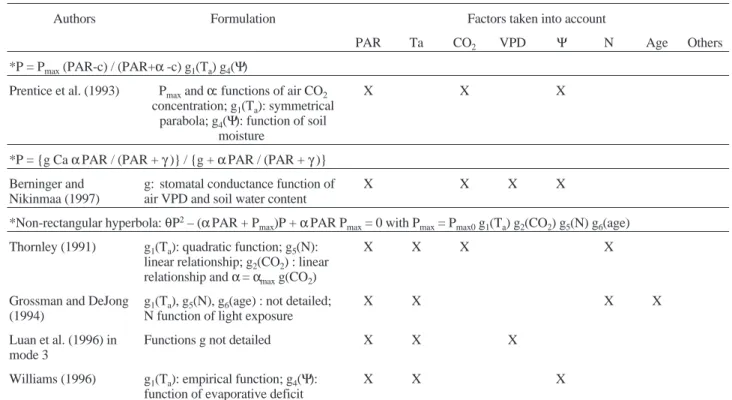
Table II. Formulations used and environmental factors taken into account in the photosynthate production submodels of the carbon-based models of individual tree growth reviewed.

Authors Formulation Factors taken into account

PAR Ta CO2 VPD Ψ N Age Others

Leaf photosynthesis not explicitly described *P =σsW or P =σsA

Promnitz (1975) P =σsWlwith constantσs

Deleuze and Houllier (1995)

id Deleuze and Houllier

(1997)

id Ågren and Axelsson

(1980)

P =σsWlwithσs=σs0f

(age, soil water and Tl)

X X X

Valentine (1985) P =σsWlwithσs=σs0f(PAR) X

Hauhs et al. (1995) id X

Perttunen et al. (1996) id X Tree

age Mäkelä and Hari (1986) P =σsAlwithσs=σs0f (PAR) X

Mäkelä (1997) P =σsWswithσs=σs0f(PAR)f(Hc) X

*P =εcPARa

West (1993) P =εcPARawith constantεc X

Takenaka (1994) id X

Kellomäki and Starndman (1995)

id X

Sorrensen et al. (1993) P =εcPARawithεc= f

(relative tree height)

X Wermelinger et al.

(1991)

P = Dem[1–exp(–εcPARa/Dem)] and

εc= f(age)

X (X) X

*P = WUE E

de Reffye et al. (1997) P = WUE E (X) (X) (X) (X)

Empirical leaf photosynthesis formulation

*Rectangular hyperbola : P = Pmax[αPAR / (αPAR + Pmax)] g1(Ta) g2(CO2) g3(VPD) g4(Ψ) g5(N) g6(age)

Rauscher et al. (1990); see Host et al. (1990b)

g1(Ta): defined for 8 temperature

classes

g6(age):αand Pmaxdefined for each

age class

X X X

Zhang et al. (1994) g1(Ta): parabolic function; g4(Ψ):

linear function under thresholdΨ, g6(age): multiplier for each age class;

(g1, g4and g6applied to Pmax);

α=αmaxg1(Ta)

carbon demand (Dem), PAR absorbed by the foliage, and an age-dependent conversion coefficientεc, as:

P= Dem. [1 – exp(–εcPARa/ Dem)]. (4) In this case, carbon uptake is sink-dependent (i.e. a function of carbon demand). Nitrogen supply indirectly influences photosynthate production in this model be-cause nitrogen restriction would have a negative feed-back on carbon demand.

However, for all these models,σsorεcis not explicitly influenced by environmental variables and rarely by leaf status variables (table II). Generally, such a simple treat-ment of photosynthate production is deliberate since these models were designed (i) to simulate tree growth under well-characterised environmental conditions, or (ii) to address very specific aspects of plant growth, e.g. to test a postulated partitioning function. Nevertheless, such a simple treatment of photosynthate production is

Authors Formulation Factors taken into account

PAR Ta CO2 VPD Ψ N Age Others

*P = Pmax(PAR-c) / (PAR+α-c) g1(Ta) g4(Ψ)

Prentice et al. (1993) Pmaxandα: functions of air CO2

concentration; g1(Ta): symmetrical

parabola; g4(Ψ): function of soil

moisture

X X X

*P = {g CaαPAR / (PAR +γ)} / {g +αPAR / (PAR +γ)} Berninger and

Nikinmaa (1997)

g: stomatal conductance function of air VPD and soil water content

X X X X

*Non-rectangular hyperbola:θP2_{– (}α_{PAR + P}

max)P +αPAR Pmax= 0 with Pmax= Pmax0g1(Ta) g2(CO2) g5(N) g6(age)

Thornley (1991) g1(Ta): quadratic function; g5(N):

linear relationship; g2(CO2) : linear

relationship andα=αmaxg(CO2)

X X X X

Grossman and DeJong (1994)

g1(Ta), g5(N), g6(age) : not detailed;

N function of light exposure

X X X X

Luan et al. (1996) in mode 3

Functions g not detailed X X X

Williams (1996) g1(Ta): empirical function; g4(Ψ):

function of evaporative deficit

X X X

*The Lohammar (1980) formulation: P = (Ca– Cc): (rs+ rm) with rs= rsmaxf1(PAR) g3(VPD) g4(Ψ) and rm= rmmaxf1(PAR) g1(Ta) g5(N)

g6(age) g7(Mg) g8(O3)

Weinstein et al. (1992); Weinstein and Yanai (1994)

g4(Ψ) : actually function of soil water

Determination of Ccnot detailed

X X X X X X Mg, O3

Mechanistic leaf photosynthesis formulation Farquhar’s model P = min (Pc, Pj)

Pc= f (Vcmax, Rd, Ci, T) and Pj= f (Jmax, Rd, PAR, Ci, T) with Vcmax, Jmax, Rdfunction of N and T

Webb et al. (1991) stomatal conductance = f (Ψ, CO2,

VPD, PAR)

X X X X X

Luan et al. (1996) in mode 4

Computation of stomatal conductance not detailed

X X X X

Balandier et al. (2000) Ci/Cc= f (PAR) X X X X

NB: The model of Escobar-Gutiérrez et al. [29] uses measured photosynthesis as an input; Luan et al. [71] in mode 2 use an hyperbolic light response curve but its equation is not detailed.

sometimes not consistent with the objectives of the tree growth models. For instance, the major objective of the model of Deleuze and Houllier [23] was to describe ra-dial and height growth for trees and to extrapolate tree growth to varying conditions. However, such an extrapo-lation to different environments should be done with ex-treme caution since the model uses a constant specific leaf activity that is not influenced by climatic parameters and leaf state.

Only three models reviewed [73, 93, 133] expressly state the effect of an environmental parameter in the con-text of this approach. The leaf specific activity approach was used in these models of Scots pine tree growth to compute photosynthate production as a function of the local radiation regime. In this case, the leaf specific ac-tivity is modulated by a so-called photosynthetic light ra-tio f(PAR) (i.e. the rara-tio between the actual leaf specific activity σs observed in a given shaded environment within the tree foliage and the leaf specific activityσs0 ex-hibited in sunlit conditions), so that:

P=σsWs (5) with:

σs=σs0f(PAR) (6) where f(PAR) is not directly a function of PAR but a function of the leaf area index above a given location.

3.1.1.2. Empirical modelling of leaf photosynthesis

Most tree growth models simulate leaf photosynthesis by empirical relationships that include sensitivity to some environmental variables (table II). Typically, leaf photosynthesis P is represented as:

P = Pmaxf(PAR) g1(Ta) g2(Ca) g3(VPD) g4(Ψ) g5(N) g6(age) (7) where Pmaxis the maximum photosynthetic rate observed at high leaf irradiance PAR and in optimal environmental conditions, f(PAR) is the key empirical function of leaf irradiance, and gi’s are multiplicative functions that ac-count for the effects of air temperature (Ta), air CO2 con-centration (Ca), air water vapour pressure deficit (VPD), plant water potential (Ψ.) or soil moisture, leaf nitrogen content (N) and leaf age. Pmaxgenerally depends on light regime [10]. The most common functions for f(PAR) en-countered in the models reviewed are the rectangular [44, 102, 147] and non rectangular [40, 128] hyperbolae. The parameters used in these relationships (table II) are gen-erally physiologically sound (e.g. the initial slope of the hyperbolic function represents quantum yield).

An alternative, empirical approach is used in the model TREGRO [139]. In this case, leaf photosynthesis

P is computed using the equation form of Lohammar etal.

[70]:

P = (Ca– Cc) / (rs+ rm) (8a) with:

rs= rsmaxf1(PAR) g1(Ψ) g2(VPD) (8b)

rm= rmmaxf1(PAR) g1(Ta) g2(y) g3(N) g4(Mg) g5(ozone) (8c) where Caand Ccare the CO2concentrations in ambient air and at the carboxylation sites, respectively, and rsand

rm are the stomatal and mesophyll resistances to CO2 transfer, respectively. Environmental variables are taken into account when computing stomatal and mesophyll resistances. However, this sole equation is not sufficient to determine P since Ccis not a constant. Because the au-thors do not explain how Ccis computed or prescribed, it is difficult to evaluate whether the use of equation 8a is straightforward.

At least, it should be noted that the empirical photo-synthesis model used in the SICA/SIMFORG model

(ta-ble II) is coupled to a stomatal conductance model that

presents the optimal scheduling of water use during a drought period [8]. This is the sole case where a teleonomic approach is used to compute leaf gas ex-changes in the tree growth models reviewed.

3.1.1.3. Mechanistic modelling of leaf photosynthesis

The photosynthesis model proposed by Farquhar et al. [30] represents the most physiologically sound approach presently available. This model simulates the photosynthetic rate of C3 species as a function of leaf irradiance, intercellular CO2concentration and leaf tem-perature. It distinguishes two factors that can limit leaf photosynthesis P (µmol CO2m

–2_s–1_):

P = min (Pc, Pj) (9) where Pcand Pjare the photosynthetic rates limited by (i) the amount, activation state and/or kinetic properties of Rubisco, or (ii) the rate of RuP2 regeneration, respec-tively. The effect of nitrogen on photosynthesis can be easily introduced in the model because the three key pa-rameters of the model (the maximum carboxylation rate, the light-saturated rate of electron transport, and the dark respiration rate) are proportional to the amount of leaf ni-trogen on an area basis [31, 66, 68]. This latter variable can be linked to local radiation regime experienced by the leaves [67, 68]. However, predicting tree growth ac-cording to soil fertility would imply to account for tree nutrient economy (see Sect. 5.3).

Because the CO2partial pressure in sub-stomatal cavi-ties (Ci) or at the carboxylation sites is an input of Farquhar’s model, an estimate of stomatal conductance is required. The most common modules available are the multiplicative approach proposed by Jarvis [46] and the semi-empirical equation developed by Ball et al. [5] (for a review, see [117]). However, most of published tree growth models that use a mechanistic approach of photo-synthesis exhibit a crude treatment of stomatal function-ing. For instance, Ci is computed by an empirical function of PAR and Cain the model SIMWAL [65], al-though the latest version of the model can also use the Jarvis approach to compute stomatal conductance [4].

3.1.1.4. Choice of a formulation for photosynthate production: implications for model applications, parameterisation and computation requirements

Models using the specific leaf activity approach do not represent explicitly the effects of several important environmental variables and leaf characteristics on photosynthate production (table II). This restricts their ability to predict tree function beyond their initial

do-main of application (i.e. a given species, in a given loca-tion). For instance, the empirical photosynthetic light ra-tio funcra-tion f(PAR) has to be calibrated for each particular stand because it depends on both structural fac-tors (tree architecture and tree density in the stand) and biological factors (shading effect on photosynthesis and respiration for the species studied). Such a calibration would be tedious and time-consuming. Thus, if a carbon-based model of tree growth is to be used for different spe-cies and/or in contrasting environments, an explicit con-sideration of the effects of environmental constraints on leaf photosynthesis is necessary. Empirical leaf photo-synthesis models offer a good potential to analyse tree photosynthate production in response to environmental stimuli. However, when using empirical formulations, the mechanisms involved in response of photosynthetic rates to environmental variables are hidden. This is not a problem in many cases, such as when the tree growth model has been designed for a specific purpose (e.g. management of young trees for a given species under given range of environmental conditions). For other applications, empirical formulations could restrict the

Figure 4. Schematic location of the photosynthate production module of each tree growth model in a space-time domain. Each symbol corresponds to a given approach to represent photosynthate production (n: Farquhar et al.’s photosynthesis model; u: empirical formu-lation of leaf photosynthesis;s: leaf specific activity approach; e: water use efficiency approach). Numbers in symbols refer to models (see legend of figure 3; 19, 19b and 19t refer to FORDYN in its mode 4, 3 and 2, respectively).

predictive capacity of the model beyond its initial scope (e.g. tree functioning in contrasting or changing environ-mental conditions). In this context, a more mechanistic formulation of leaf photosynthesis is probably required. For instance, using the Farquhar approach in the tree seedling model of Webb [138] is consistent with the model’s objective, i.e. predicting seedling growth under increased CO2levels. However, despite its great predic-tive potential, a mechanistic approach of photosynthesis is not the panacea for modelling photosynthate produc-tion by trees. It is only required when a comprehensive understanding of photosynthetic processes is necessary (which can sometimes be the case for generalisation or educational needs) and when a complex formulation of photosynthesis is consistent with the complexity of the other modules used by the tree growth model.

Beyond their ability to explicitly represent environ-mental effect on photosynthesis and to be applied under new environmental conditions, the different formula-tions of photosynthate production have to be evaluated from a pragmatic point of view in the context of compu-tation requirements and model parameterisation. Due to the non-linearity of the leaf photosynthesis-light re-sponse, models that compute leaf photosynthesis cannot be utilised unless a physiologically sensible time step is applied. The different formulations of photosynthate production used by the models reviewed are located in a time-space domain in figure 4: this shows that models us-ing an empirical or biochemically based approach to sim-ulate the effects of environment on leaf photosynthesis are all run at a time step of one hour or less. The only ex-ceptions are the models FORSKA and ARCADIA that compute monthly or annual carbon gain using a formula-tion usually devoted to represent instantaneous leaf pho-tosynthesis. In this case, the model is parameterised from coarse scale data rather than leaf gas exchange data [97], and the formulation has not the same meaning as its origi-nal form. In addition, using an empirical or biochemi-cally based formulation of leaf photosynthesis requires a detailed description of the variations of the environmen-tal driving variables inside the canopy (vertical profiles or 3D distribution of relevant environmental variables according to the spatial representation used). In contrast, models that only assume a dependence of shading on photosynthate production (equation 5) look at longer time scales [133] or situations where the rest of environ-mental variables can be controlled. In this case, the inte-grated effect of the environmental variability can be incorporated in the input parameterσs.

Combining a temporal coarse approach (such as the leaf specific activity or conversion efficiency approach)

to a higher temporal resolution approach representing leaf photosynthesis is a good means to solve this di-lemma. Berninger and Nikinmaa [9] used this method where a high resolution model (flux model SICA) pro-vides annual photoproduction to SIMFORG. The ap-proach used by the model FORDYN [71] to simulate tree carbon gain is even more flexible. A key feature of this model is that users can choose a particular approach, among different available, to simulate photosynthate production (i.e. tree annual photosynthate production by a species-dependent hyperbolic light response curve vs. hourly or instantaneous leaf photosynthesis by a non-rectangular hyperbola or by the Farquhar’s model). Such an approach greatly enhances model versatility.

3.1.2. Representation of the distribution

of photosynthate production within the tree crown, and associated radiation transfer modules

In addition to the various ways of formulating photo-synthesis, carbon-based models simulating the growth of woody plants also differ in their representations of the spatial distribution of carbon gain within tree foliage. This is related to the way tree architecture is accounted for (Sect. 2.3) and implies the use of specific radiation transfer modules.

Whatever the method used for representing leaf distri-bution (that determines the spatial distridistri-bution of simulated carbon gain), models using the compartmental approach cannot assign carbon assimilation rates to individual shoots or leaves (table III). Most of the compartmental models reviewed simulate total carbon gain at the individual tree scale [23, 75, 100, 133], or rep-resent the vertical distribution of carbon sources within the foliage [139]. In the later case, provided that the verti-cal distribution of foliage is known, Beer’s law is applied to compute the vertical distribution of leaf irradiance and then total photosynthate production or the vertical profile of carbon gain. The photosynthetic light ratio approach (equation 5) can also be applied to simulate the effect of PAR on carbon gain as an alternative to traditional mod-ules simulating leaf irradiance effect on photosynthesis [73]. In contrast, even compartmental models would need a very detailed representation of crown structure and a complex radiation interception module if they aim to accurately represent competition between individual trees in complex forest stands (several tree species, several tree sizes). For instance, although West [142] uses a complex submodel of light interception, his compartmental model aims only at computing total car-bon gain by individual trees within a forest stand.

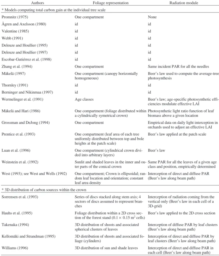
Table III. Foliage representation and radiation module used to compute photosynthetic production and its spatial distribution. Models computing whole tree carbon gain or local carbon gains within the tree crown are distinguished.

Authors Foliage representation Radiation module

* Models computing total carbon gain at the individual tree scale

Promnitz (1975) One compartment None

Ågren and Axelsson (1980) id id

Valentine (1985) id id

Webb (1991) id id

Deleuze and Houllier (1995) id id

Deleuze and Houllier (1997) id id

Escobar-Gutiérrez et al. (1998) id id

Zhang et al. (1994) One compartment Same incident PAR for all the needles

Mäkelä (1997) One compartment (canopy horizontally

homogeneous)

Beer’s law used to compute the average-tree photosynthesis

Thornley (1991) id id

Berninger and Nikinmaa (1997) id id

Wermelinger et al. (1991) Age classes Beer’s law; age-specific photosynthetic

effi-ciencies modulate effective LAI

Mäkelä and Hari (1986) One compartment (foliage distributed within

a cylindrically symetrical crown)

Photosynthetic light ratio function of leaf biomass above a given location

Grossman and DeJong (1994) One compartment Empirical data on daily light interception in

orchards used to adjust an effective LAI

Prentice et al. (1993) One compartment (leaf area of each tree

uniformly distributed between top and bole heights at the patch scale)

Beer’s law applied at the patch scale

Luan et al. (1996) One compartment (cylindrical crown

divi-ded into arbitrary layers)

Beer’s law Weinstein et al. (1992) Sunlit and shaded leaves in the inner and

ou-ter parts of the conical crown

Same PAR for all the leaves of a given age class and position, empirically determined West (1993); see West and Wells (1992) One compartment; Crown is ellipsoidal;

ran-dom leaf location and orientation; constant leaf area density

Interception of direct and diffuse PAR (Beer’s law along beam path) * 3D distribution of carbon sources within the crown

Sorrensen et al. (1993) Series of discs stacked along stem axis; 4 sectors of discs assumed to represent bran-ches

Interception of radiation coming from the vertical only (Beer’s law in each cell of a 3D-grid)

Hauhs et al. (1995) Foliage distribution within a 2D cross

sec-tion of the forest stand (0.1×0.15 m2_cells)

Beer’s law applied to the 2D cross section

Takenaka (1994) 3D distribution of shoots and associated

spherical clusters of leaves

Interception of diffuse PAR by leaf clusters (Beer’s law along beam path)

Kellomäki and Strandman (1995) 3D distribution of shoots and associated fo-liage (cylinders)

Interception of direct and diffuse PAR by leaf clusters (Beer’s law along beam path)

Williams (1996) 3D distribution of sun and shade leaves Interception of direct and diffuse PAR in

Models using the organ-based approach to simulate individual organ growth must simulate carbon gain by different tree parts (branches or growth units and associ-ated foliage clusters, or the individual leaves). Thus, these models include a light interception submodel that computes light regime for each leaf or shoot within the tree crown canopy (e.g. models ECOPHYS, WHORL and SIMWAL, Takenaka’s model, Kellomäki and Strandman’s model) (table III). Most of these models compute incoming direct and diffuse photon flux densi-ties from different elevation angles. PAR interception is then computed by the turbid medium analogy, i.e. apply-ing Beer’s law to leaf cluster volumes associated to each shoot or tree parts according to leaf area density, and leaf orientation and distribution [51, 123]. In the case of the model WHORL, interception of only vertically incoming radiation is considered, which is a deterrent for an accu-rate representation of local radiation regimes within the tree crown [120]. In contrast to models using the turbid medium analogy, the model ECOPHYS simulates direct and diffuse PAR interception by each individual leaf us-ing a geometrical approach. A mixed, turbid me-dium/geometric approach was used in SIMWAL where a geometric model is used for young trees exhibiting a neg-ligible self-shading between leaves, and Beer’s law is ap-plied for bigger trees [4]. Some organ-based models use cruder approaches. In LIGNUM [93], the photosynthetic light ratio approach is used rather than a radiation trans-fer module.

3.1.3. Summary

Tree growth models exhibit different formulations for photosynthate production and different representations of the spatial variability of carbon gain. However, the use of a particular photosynthesis function does not require

or preclude a particular method for representing the spa-tial distribution of carbon gain. For instance, the model LIGNUM [93] uses the empirical photosynthetic light ra-tio approach to simulate annual carbon gain; the model ECOPHYS [102] simulates leaf photosynthesis with a rectangular hyperbola function; and the model SIMWAL [4] uses the mechanistic Farquhar model to simulate the leaf photosynthetic rate. However, all these models use an organ-based approach and represent the 3D–distribu-tion of carbon gain at the shoot- or leaf-level. Thus, de-spite different representations of carbon assimilation, the models all exhibit a good potential to analyse in details structure-function relationships involved in tree architec-ture dynamics. Therefore, model objectives strongly constrain the method used to represent the spatial distri-bution of carbon gain (e.g. computation of total carbon gain for simulating wood production vs. computation of the 3D-distribution of carbon gain at the organ scale for predicting architecture dynamics), and constrain the choice of a photosynthesis formulation to a weaker ex-tent (use of empirical photosynthate production modules to describe the tree functioning in the long term vs. use of mechanistic leaf photosynthesis modules to provide ra-tionales for predicting tree responses to future environ-mental changes).

3.2. Modelling respiration

Net production of plant biomass strongly depends on carbon losses resulting from respiration. For example, in herbaceous plants, respiratory losses were estimated to be 50% of the photosynthetically fixed carbon [3]. Simi-larly, respiration losses may account for 40–60% of gross photosynthesis of cool temperate forests [122]. How-ever, reliable measurements of whole-plant carbon

Authors Foliage representation Radiation module

Perttunen et al. (1996) 3D distribution of tree segments and

associated foliage

PLR function of leaf biomass above a given location

Rauscher et al. (1990) 3D geometric model of tree crown : size,

orientation and area of each leaf specified

Direct and diffuse PAR on both sunlit and shaded leaf portion (geometric model)

Balandier et al. (2000) mixed 3D geometric/turbid medium

approach

Direct and diffuse PAR interception by each leaf (geometric model for young trees ; Beer’s law along beam path for old trees)

NB: The model of de Reffye et al. [103] computes photosynthesis indirectly by a tree hydraulic architecture approach that does not use foliage representa-tion.

balance and its components are scarce. Consequently, most carbon-based models of tree growth use a simpli-fied, theoretical representation of respiratory processes, i.e. either a two-component approach or a global, non-ex-plicit treatment of respiration (table IV).

3.2.1. The two-component model

It is widely accepted that plant respiration has at least two components, growth and maintenance. Growth res-piration is defined as the resres-piration associated with the

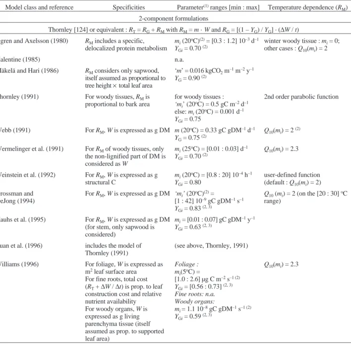
Table IV. The respiration submodels of the 27 models reviewed. W : dry matter (DM); R_T: total respiration; R_Mor R’_M: maintenance-associated component of R_T; R_G, or R’_G: growth-associated component of R_T; P : gross photosynthesis; n.a. : not available. Unless oth-erwise specified, W stands for total DM (living + inert); R_T, R_M, R_G, W and P are expressed as equivalent C units.

Model class and reference Specificities Parameter(1)_{ranges [min : max] Temperature dependence (R} M)

2-component formulations

Thornley [124] or equivalent : RT= RG+ RMwith RM= m · W and RG= [(1 – YG) / YG] · (∆W / t)

Ågren and Axelsson (1980) RMincludes a specific,

delocalized protein metabolism

mi(20oC)(2)= [0.3 : 1.2] 10–3d–1

YGi= 0.70(2)

winter woody tissue : mi= 0;

other cases : Q10(mi) = 2

Valentine (1985) n.a.

Mäkelä and Hari (1986) RMconsiders only sapwood,

itself assumed as proportional to tree height×total leaf area

‘m’ = 0.016 kgCO2m–1m–2y–1

YG= 0.90(2)

Thornley (1991) For woody tissues, RMis

proportional to bark area

for woody tissues :

‘mi’ (20oC) = 0.5 gC m–2d–1

else: mi(20oC) = 0.001 d–1

YGi= 0.75

2nd order parabolic function

Webb (1991) For RM, W is expressed as g DM m (20oC) = 0.33 gC gDM–1d–1

YG= 0.75(2)

Q10(mi) = 2(2)

Wermelinger et al. (1991) For RMof woody tissues, only

the non-lignified part of DM is considered as W

mi(25oC) = [0.01 : 0.03] d–1

YGi= 0.70(2)

Q10(mi) = 2.3

Weinstein et al. (1992) For RM, W is expressed as g

structural C mi(20oC) = [0.8 : 20] 10–4h–1 YGi= 0.80 user-defined function (default : Q10(mi) = 2) Grossman and DeJong (1994) For RM, W is expressed as g DM ‘mi’ (20oC)(2)= [1 : 42] 10–9_{gC gDM}–1_s–1 YGi= 0.83(2, 3) Q10(mi) = 2 (on the [20 : 30]oC range) Hauhs et al. (1995) For RM, W is expressed as g DM

(for stem, only sapwood is considered)

mi= [0.01 : 0.07] gC gDM–1y–1

YGi= 0.63(2, 3)

Luan et al. (1996) includes the model of

Thornley (1991)

(see above, Thornley, 1991)

Williams (1996) For foliage, W is expressed as

m2_{leaf surface area}

For fine roots, total cost (RT+∆W /∆t) is prop. to leaf

construction cost and relative nutrient availability

For woody organs, W is expressed as g living parenchyma tissue (itself assumed as prop. to supported leaf area)

Foliage : mi(5oC) =

[1.0 : 2.6] µg C m–2_s–1 (2)

YGi= [0.56 : 0.73](2, 3)

Fine roots: n.a. Woody organs:

mi= 1.1 10–8gC gDM–1s–1 (2)

YGi= 0.59(2, 3)

synthesis of new biomass, while maintenance respiration is defined as that required for maintenance and turnover of existing biomass [2, 3, 48, 79, 107, 124]. Most of the

tree growth models reviewed here use one of the two formalisms that were developed concurrently in 1970, one by McCree and the other by Thornley. Each formulation

Model class and reference Specificities Parameter(1)_{ranges [min : max] Temperature dependence (R} M)

Deleuze and Houllier (1997) For RM, W is expressed as:

g DM for leaves and roots m2_{bark area for stem;}

RGis ignored for stem

‘mi’ = 0.1 gC gDM–1y–1for

leaves, roots;

‘mi’ = 10 gC m–2y–1for stem

YGi= 0.92(2, 3)for leaves, roots

Berninger and Nikinmaa (1997) mi: n.a.

YGi= 0.80

Q10(mi) = 2

Mäkelä (1997) For RM, W is expressed

as g DM

‘mi’ = [0.02 : 0.2] gC gDM–1y–1

YGi= 0.75(2)

Escobar-Gutiérrez et al. (1998) For RM, W is expressed

as g structural C

mi= 0.016 d–1

YGi= 0.75

Balandier et al. (2000) For RM, W is expressed

as g DM;

Fine root RGimplicitly

includes turnover losses

‘mi’ =

[6 : 50] 10–4_{g CO}

2gDM–1h–1

YGi= 0.50 for fine roots

YGi= 0.75 for other organs

Q10(mi) = 2

McCree (1970) or equivalent RT= R’G+ R’Mwith R’M= c⋅ W and R’G= (1−YG)⋅ P

Promnitz (1975) For R’M, W is expressed

as g DM

‘ci’ = 2 mg CO2gDM–1h–1

YGi: n.a.

Rauscher et al. (1990) diurnal net photosynthesis used in calculation of R’G ci= 0.015 d–1 YGi= 0.75(2) user-defined Zhang et al. (1994) ‘ci’(20oC)(2)= [1.6 : 22] 10–5h–1 YGi= [0.67 : 0.73](2, 3)

simplified Arrhenius function Deleuze and Houllier (1995) For the stem, RMis

proportional to bark area

ci= 0.1 y–1for leaves, roots;

‘ci’ = 10 gC m–2y–1for stem

YGi= 0.81(2)

One-component formulation (RGignored or implicit): R = k⋅ W

Prentice et al. (1993) Only sapwood maintenance respiration computed, using the pipe model

k: n.a. Q10= 2.3

Takenaka (1994) only leaf maintenance cost is

explicitly computed.

kleaf= 0.25 y–1

Perttunen et al. (1996) ki= [0.02 : 0.2] y–1

Respiration ignored or implicitly taken into account in a global light conversion efficiency (see table II) Sorrensen-Cothern et al. (1993)

West (1993)

Kellomäki and Strandman (1995)

De Reffye et al. (1997a,b)

(1)_{Indexed parameters refer to specific tissue components (e.g. branches, stems, coarse roots...).} (2)_{Recalculated from related parameter values.}

(3)_{Recalculated assuming a DM C content of f}

c= 0.42 gC gDM–1.