HAL Id: hal-01112160
https://hal.inria.fr/hal-01112160
Submitted on 2 Feb 2015
HAL is a multi-disciplinary open access
archive for the deposit and dissemination of
sci-entific research documents, whether they are
pub-lished or not. The documents may come from
teaching and research institutions in France or
abroad, or from public or private research centers.
L’archive ouverte pluridisciplinaire HAL, est
destinée au dépôt et à la diffusion de documents
scientifiques de niveau recherche, publiés ou non,
émanant des établissements d’enseignement et de
recherche français ou étrangers, des laboratoires
publics ou privés.
Characterizing polynomial time complexity of stream
programs using interpretations
Hugo Férée, Emmanuel Hainry, Mathieu Hoyrup, Romain Péchoux
To cite this version:
Hugo Férée, Emmanuel Hainry, Mathieu Hoyrup, Romain Péchoux. Characterizing polynomial time
complexity of stream programs using interpretations. Theoretical Computer Science, Elsevier, 2015,
585, pp.41-54. �10.1016/j.tcs.2015.03.008�. �hal-01112160�
Characterizing polynomial time complexity of stream
programs using interpretations
Hugo F´er´eea,c, Emmanuel Hainrya,c, Mathieu Hoyrupb,c, Romain P´echouxa,c
aUniversit´e de Lorraine, Nancy, France bInria Nancy - Grand Est, Villers-l`es-Nancy, France
cProject-team CARTE, LORIA, UMR7503
Abstract
This paper provides a criterion based on interpretation methods on term rewrite systems in order to characterize the polynomial time complexity of sec-ond order functionals. For that purpose it introduces a first order functional stream language that allows the programmer to implement second order func-tionals. This characterization is extended through the use of exp-poly interpre-tations as an attempt to capture the class of Basic Feasible Functionals (bff). Moreover, these results are adapted to provide a new characterization of poly-nomial time complexity in computable analysis. These characterizations give a new insight on the relations between the complexity of functional stream pro-grams and the classes of functions computed by Oracle Turing Machine, where oracles are treated as inputs.
Keywords:
Stream Programs, Type-2 Functionals, Interpretations, Polynomial Time, Basic Feasible Functionals, Computable Analysis, Rewriting
1. Introduction
Lazy functional languages like Haskell allow the programmer to deal with co-inductive datatypes in such a way that co-inductive objects can be evaluated by finitary means. Consequently, computations over streams, that is infinite lists, can be performed in such languages.
A natural question arising is the complexity of the programs computing on streams. Intuitively, the complexity of a stream program is the number of reduction steps needed to output the n first elements of a stream, for any n. However the main issue is to relate the complexity bound to the input structure. Since a stream can be easily identified with a function, a good way for solving such an issue is to consider computational and complexity models dealing with functions as inputs.
In this perspective, we want to take advantage of the complexity results obtained on type-2 functions (functions over functions), and in particular on
set Unary Oracle Turing Machine (uotm), machines computing functions with oracles taking unary inputs, as our main computational model. This model is well-suited in our framework since it manipulates functions as objects with a well-defined notion of complexity. uotm are a refinement of Oracle Turing Machines (otm) on binary words which correspond exactly to the bff algebra in [3] under polynomial restrictions. uotm are better suited than otm to study stream complexity with a realistic complexity measure, since in the uotm model accessing the nth
element costs n transitions whereas it costs log(n) in the otm model.
The Implicit Computational Complexity (ICC) community has proposed characterizations of otm complexity classes using function algebra [3, 4] and type systems [5,6] or recently as a logic [7].
These latter characterizations are inspired by former characterizations of type-1 polynomial time complexity based on ramification [8, 9]. This line of research has led to new developments of other ICC tools and in particular to the use of (polynomial) interpretations in order to characterize the classes of functions computable in polynomial time or space [10,11].
Polynomial interpretations [12,13] are a well-known tool used to show the termination of first order term rewrite systems. This tool has been adapted into variants, like quasi-interpretations and sup-interpretation [14], that allow the programmer to analyze program complexity. In general, interpretations are restricted to inductive data types and [15] was a first attempt to adapt such a tool to co-inductive data types including stream programs. In this paper, we introduce a second order variation of this interpretation methodology in order to constrain the complexity of stream program computation and we obtain a characterization of uotm polynomial time computable functions. Using this characterization, we can analyze functions of this class in an easier way based on the premise that it is practically easier to write a first order functional pro-gram on streams than the corresponding Unary Oracle Turing Machine. The drawback is that the tool suffers from the same problems as polynomial inter-pretation: the difficulty to automatically synthesize the interpretation of a given program (see [16]). As a proof of versatility of this tool, we provide a partial characterization of the bff class (the full characterization remaining open), just by changing the interpretation codomain: for that purpose, we use restricted exponentials instead of polynomials in the interpretation of a stream argument. A direct and important application is that second order polynomial inter-pretations on stream programs can be adapted to characterize the complexity of functions computing over reals defined in Computable Analysis [17]. This approach is a first attempt to study the complexity of such functions through static analysis methods.
This paper is an extended version of [18] with complete proofs, additional examples and corrections.
Outline of the paper.
In Section2, we introduce (Unary) Oracle Turing Machines and their com-plexity. In Section3, we introduce the studied first order stream language. In
Section 4, we define the interpretation tools extended to second order and we provide a criterion on stream programs. We show our main characterization re-lying on the criterion in Section5. Section6develops a new application, which was only mentioned in [18], to functions computing over reals.
2. Polynomial time Oracle Turing Machines
In this section, we will define a machine model and a notion of complexity relevant for stream computations. This model (uotm) is adapted from the Or-acle Turing Machine model used by Kapron and Cook in their characterization of Basic Feasible functionals (bff) [3]. In the following, |x| will denote the size of the binary encoding of x ∈ N, namely dlog2(x)e.
Definition 1 (Oracle Turing Machine). An Oracle Turing Machine (denoted by otm) M with k oracles and l input tapes is a Turing machine with, for each oracle, a state, one query tape and one answer tape.
Whenever M is used with input oracles F1, . . . Fk : N −→ N and arrives on the oracle state i ∈ {1, . . . , k} and if the corresponding query tape contains the binary encoding of a number x, then the binary encoding of Fi(x) is written on the corresponding answer tape. It behaves like a standard Turing machine on the other states.
We now introduce the unary variant of this model, which is more related to stream computations as accessing the n-th element takes at least n steps (whereas it takes log(n) steps in otm. See example2 for details).
Definition 2 (Unary Oracle Turing Machine). A Unary Oracle Turing Ma-chine (denoted uotm) is an otm where numbers are written using unary no-tation on the query tape, i.e. on the oracle state i, if w is the content of the corresponding query tape, then Fi(|w|) is written on the corresponding answer tape.
Definition 3 (Running time). In both cases (otm and uotm), we define the cost of a transition as the size of the answer of the oracle, in the case of a query, and 1 otherwise.
In order to introduce a notion of complexity, we have to define the size of the inputs of our machines.
Definition 4 (Size of a function). The size |F | : N −→ N of a function F : N −→ N is defined by:
|F |(n) = max k≤n|F (k)|
Remark 1. This definition is different from the one used in [3] (denoted here by ||.||). Indeed, the size of a function was defined by ||F ||(n) = max|k|≤n|F (k)|, in other words, ||f ||(n) = |f |(2n− 1). The reason for this variation is that in an
following) than to a function, since it can access easily its first n elements but not its (2n)th element which is the case in an otm. In particular, this makes the size function computable in polynomial time (with respect to the following definitions).
The size of an oracle input is then a type-1 function whereas it is an integer for standard input. Then, the notion of polynomial running time needs to be adapted.
Definition 5 (Second order polynomial). A second order polynomial is a polynomial generated by the following grammar:
P := c | X | P + P | P × P | Y hP i
where X represents a zero order variable (ranging over N), Y a first order variable (ranging over N −→ N), c a constant in N and h−i is a notation for the functional application.
Example 1. P (Y1, Y2, X1, X2) = (Y1hY1hX1i × Y2hX2ii)2 is a second order polynomial.
The following lemma shows that the composition of polynomials is well be-haved.
Lemma 1. If the first order variables of a second order polynomial are replaced with first order polynomials, then the resulting function is a first order polyno-mial.
Proof. This can be proved by induction on the definition of a second order polynomial: this is true if P is constant or equal to a zero order variable and also if P is a sum, a multiplication or a composition with type-1 variable, since polynomials are stable under these operators.
In the following, P (Y1, . . . , Yk, X1, . . . , Xl) will denote a second order poly-nomial where each Yi represents a first order variable, and each Xi a zero order variable.
This definition of running time is directly adapted from the definition of running time for otms.
Definition 6 (Polynomial running time). Anuotm M operates in time T : (N −→ N)k −→ Nl−→ N if for all inputs x
1, . . . xl : N and F1, . . . Fk : N −→ N, the sum of the transition costs before M halts on these inputs is less than T (|F1|, . . . , |Fk|, |x1|, . . . , |xl|).
A function G : (N −→ N)k−→ Nl−→ N is uotm computable in polynomial time if there exists a second order polynomial P such that G is computed by an uotm in time P .
Lemma 2. The set of polynomial time uotm computable functions is strictly included in the set of polynomial time otm computable functions (proved to be equal to the bff algebra [3]):
Proof. In order to transform a uotm into an otm computing the same func-tional, we have to convert the content of the query tape from the word w (rep-resenting |w| in unary) into the binary encoding of |w| before each oracle call. This can be done in polynomial time in |w| and we call Q this polynomial. In both cases, the cost of the transition is |F (|w|)|, so the running time of both machines is the same, except for the conversion time. If the computation time of the uotm was bounded by a second order polynomial P , the size of the con-tent of the query is at most P (|F |) at each query, so the additional conversion time is at most Q(P (|F |)) for each query and there are at most P (|F |) queries. Thus, the conversion time is also a second order polynomial in the size of the inputs, and the computation time of the otm is also bounded by a second order polynomial in |F |. Finally, since ||F || bounds |F |, the computation time is also bounded by the same polynomial in ||F ||, so F is in bff.
Example 2. The function G : (N −→ N) × N −→ N defined by G(F, x) = F (|x|) = F (dlog2(x)e) is uotm computable in polynomial time. Indeed, it is computed by the function which copies the input word representing x on the query tape before entering the query state before returning the content of the answer tape as output. Its running time is bounded by 2 × (|x| + |F |(|x|)).
However H(F, x) = F (x) is not uotm computable in polynomial time, be-cause it would require to write x in unary on the query tape, which costs 2|x|. Nonetheless, H is in bff because an otm only has to write x in binary, and the oracle call costs |F (x)| ≤ ||F ||(|x|).
3. First order stream language 3.1. Syntax
In this section, we define a simple Haskell-like lazy first order functional language with streams.
F will denote the set of function symbols, C the set of constructor symbols and X the set of variable names. A program is a list of definitions D given by the grammar in Figure1:
p ::= x | c p1 . . . pn | p : y (Patterns) e ::= x | t e1 . . . en (Expressions) d ::= f p1 . . . pn= e (Definitions)
where x, y ∈ X , t ∈ C ∪ F , c ∈ C \ {:} and f ∈ F and c, t and f are symbols of arity n.
Throughout the paper, we call closed expression any expression without variables.
The stream constructor : ∈ C is a special infix constructor of arity 2. In a stream expression h : t, h and t are respectively called the head and the tail of the stream.
We might use other infix or postfix constructors or function symbols in the following for ease of readability.
In a definition f p1 . . . pn= e, all the variables of e appear in the patterns pi. Moreover patterns are non overlapping and each variable appears at most once in the left-hand side. This entails that programs are confluent. In a program, we suppose that all pattern matchings are exhaustive. Finally, we only allow patterns of depth 1 for the stream constructor (i.e. only variables appear in the tail of a stream pattern).
Remark 2. This is not restrictive since a program with higher pattern match-ing depth can be easily transformed into a program of this form usmatch-ing extra function symbols and definitions. We will prove in Proposition1that this mod-ification does not alter our results on polynomial interpretations.
3.2. Type system
Programs contain inductive types that will be denoted by Tau. For example, unary integers are defined by:
data Nat = 0 | Nat +1 (with 0, +1 ∈ C), and binary words by:
data Bin = Nil | 0 Bin | 1 Bin.
Consequently, each constructor symbol comes with a typed signature and we will use the notation c :: T to denote that the constructor symbol c has type T. For example, we have 0 :: Nat and +1 :: Nat -> Nat. Note that in the following, given some constants n, k, . . . ∈ N, the terms n, k,. . . denote their encoding as unary integers in Nat.
Programs contain co-inductive types defined by data [Tau] = Tau : [Tau] for each inductive type Tau. This is a distinction with Haskell, where streams are defined to be both finite and infinite lists, but not a restriction since finite lists may be defined in this language and since we are only interested in showing properties of total functions (i.e. an infinite stream represents a total function). In the following, we will write Tkfor T -> T -> ...-> T (with k occurrences of T).
Each function symbol f comes with a typed signature that we restrict to be either f::[Tau]k -> Taul -> Tau or f::[Tau]k -> Taul -> [Tau], with k, l ≥ 0.
Throughout the paper, we will only consider well-typed programs where the left-hand side and the right-hand side of a definition can be given the same type using the simple rules of Figure2 with A, Ai ∈ {Tau, [Tau]}. Γ is a typing basis for every variable, constructor and function symbol (we assume that each variable is used in at most one definition, for the sake of simplicity).
Γ(x) = A Γ ` x :: A x ∈ X ∪ C ∪ F ∀(f p1. . . pn= e) ∈ D, Γ ` e :: A ∀i, Γ ` pi:: Ai Γ ` f :: A1 -> . . . -> An -> A f ∈ F Γ ` t :: A1 -> . . . -> An -> A ∀i ∈ {1, . . . , n}, ei :: Ai Γ ` t e1. . . en:: A t ∈ C ∪ F
Figure 2: Typing rules
3.3. Semantics
Lazy values and strict values are defined in Figure3:
lv ::= e1: e2 (Lazy value) v ::= c v1 . . . vn (Strict value)
Figure 3: Values and lazy values
where e1, e2are closed expressions and c belongs to C \ {:}. Lazy values are stream expressions with the constructor symbol : at the top level whereas strict values are expressions of inductive type where only constructor symbols occur and are used to deal with fully evaluated elements.
Moreover, let S represent the set of substitutions σ that map variables to expressions. As usual the result of applying the substitution σ to an expression e is denoted σ(e).
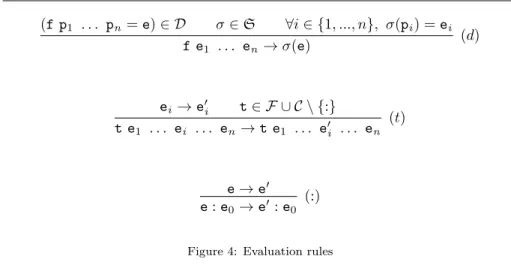
(f p1 . . . pn = e) ∈ D σ ∈ S ∀i ∈ {1, ..., n}, σ(pi) = ei f e1 . . . en→ σ(e) (d) ei→ e0i t ∈ F ∪ C \ {:} t e1 . . . ei . . . en → t e1 . . . e0i . . . en (t) e → e0 e : e0→ e0 : e0 (:)
Figure 4: Evaluation rules
We will write e →n
e0 if there exist expressions e1, . . . , en−1 such that e → e1· · · → en−1 → e0. Let →∗ denote the transitive and reflexive closure of →. We write e →! e0 if e is normalizing to the expression e0, i.e. e →∗ e0 and there is no e00 such that e0 → e00. We can show easily wrt the evaluation rules (and because definitions are exhaustive) that given a closed expression e, if e →! e0 and e :: Tau then e0 is a strict value, whereas if e →!e0 and e :: [Tau] then e0 is a lazy value. Indeed the (t) rule of Figure4 allows the reduction of an expression under a function or constructor symbol whereas the (:) rule only allows reduction of a stream head (this is why stream patterns of depth greater than 1 are not allowed in a definition).
These reduction rules are not deterministic but a call-by-need strategy could be defined to mimic Haskell’s semantic.
The following function symbols are typical stream operators and will be used further.
Example 3. s !! n computes the (n + 1)thelement of the stream s: !! :: [Tau] -> Nat -> Tau
(h:t) !! (n+1) = t !! n (h:t) !! 0 = h
Example 4. tln s n drops the first n + 1 elements of the stream s: tln :: [Tau] -> Nat -> [Tau]
tln (h:t) (n+1) = tln t n tln (h:t) 0 = t
4. Second order polynomial interpretations
In the following, we will call a positive functional any function of type (N −→ N)k −→ Nl
Given a positive functional F : ((N −→ N)k× Nl) −→ T , the arity of F is k + l.
Let > denote the usual ordering on N and its standard extension to N −→ N, i.e. given F, G : N −→ N, F > G if ∀n ∈ N \ {0}, F (n) > G(n) (the comparison on 0 is not necessary since we will only use strictly positive inputs).
We extend this ordering to the set of positive functionals of arity k + l by: F > G if
∀y1, . . . yk ∈ N −→↑N, ∀x1. . . xl ∈ N \ {0}, F (y1, . . . yk, x1, . . . , xl) > G(y1, . . . yk, x1, . . . , xl) where N −→↑N is the set of increasing functions on positive integers.
Definition 7 (Monotonic positive functionals). A positive functional is monotonic if it is strictly increasing with respect to each of its arguments. Definition 8 (Types interpretation). The type signatures of a program are interpreted as types this way:
• an inductive type Tau is interpreted as N • a stream type [Tau] is interpreted as N −→ N
• an arrow type A -> B is interpreted as the type TA−→ TB if A and B are respectively interpreted as TA and TB.
Definition 9 (Assignment). An assignment is a mapping of each function symbol f :: A to a monotonic positive functional whose type is the interpretation of A.
An assignment can be canonically extended to any expression in the program:
Definition 10 (Expression assignment). The assignment is defined on con-structors and expressions this way:
• LcM(X1, . . . , Xn) = Pn i=1Xi+ 1, if c ∈ C \ {:} is of arity n. • ( L:M(X, Y )(0) = X L:M(X, Y )(Z + 1) = 1 + X + Y hZ i
• LxM = X , if x is a variable of type Tau, i.e. we associate a unique zero order variable X in N to each x ∈ X of type Tau.
• LyM(Z ) = Y hZ i, if y is a variable of type [Tau], i.e. we associate a unique first order variable Y : N −→ N to each y ∈ X of type [Tau].
Remark 3. For every expression e,LeM is a monotonic positive functional, since it is true for function symbols, for constructors, and the composition of such functionals is still monotonic positive.
Example 5. The stream constructor : has type Tau -> [Tau] -> [Tau]. Con-sequently, its assignmentL:M has type (N × (N −→ N)) −→ (N −→ N). Let us consider the expression p : (q : r), with p, q, r ∈ X , we obtain that:
Lp : (q : r)M = L:M(LpM, Lq : rM) = L:M(LpM, L:M(LqM, LrM)) = L:M(P, L:M(Q, R)) = F (R, Q, P )
where F ∈ ((N −→ N) × N2
) −→ (N −→ N) is the positive functional such that: • F (R, Q, P )(Z + 2) = 1 + P +L:M(Q, R)(Z + 1) = 2 + P + Q + R(Z ) • F (R, Q, P )(1) = 1 + P +L:M(Q, R)(0) = 1 + P + Q
• F (R, Q, P )(0) = P
Lemma 3. The assignment of an expression e defines a positive functional in the assignment of its free variables (and an additional type-0 variable if e :: [Tau]).
Proof. By structural induction on expressions. This is the case for variables and for the stream constructor, the inductive constructors are additive, and the assignments of function symbols are positive (the composition of a positive functional with positive functional being a positive functional).
Definition 11 (Polynomial interpretation). An assignment L−M of the function symbols of a program defines an interpretation if for each definition f p1. . . pn = e ∈ D,
Lf p1. . . pnM > LeM.
Furthermore,LfM is polynomial if it is bounded by a second order polynomial. In this case, the program is said to be polynomial.
The following programs will be used further and have polynomial interpre-tations:
Example 6. The sum over unary integers: plus :: Nat -> Nat -> Nat
plus 0 b = b
plus (a+1) b = (plus a b)+1
plus admits the following (polynomial) interpretation: LplusM(X1, X2) = 2 × X1+ X2
Indeed, we check that the following inequalities are satisfied: Lplus 0 bM = 2 + B > B = LbM
Example 7. The product of unary integers: mult :: Nat -> Nat -> Nat
mult 0 b = 0
mult (a+1) b = plus b (mult a b)
The following inequalities show thatLmultM(X1, X2) = 3 × X1× X2 is an inter-pretation for mult:
Lmult 0 bM = 3 × L0M × LbM = 3 × B > 1 = L0M Lmult (a+1) bM = 3 × A × B + 3 × B
> 2 × B + 3 × A × B =Lplus b (mult a b)M
Note that these interpretations are first order polynomials because plus and mult only have inductive arguments.
Example 8. The function symbol !! defined in Example3admits an interpre-tation of type ((N −→ N) × N) −→ N defined by:
L!!M(Y , N ) = Y hN i.
Indeed, we check that:
L(h:t) !! (n+1)M = Lh:tM(LnM + 1) = 1 + LhM + LtM(LnM) > LtM(LnM) = Lt !! nM L(h:t) !! 0M = Lh:tM(L0M) = Lh:tM(1) = 1 + LhM + LtM(0) > LhM
Example 9. The function symbol tln defined in Example 4 admits an inter-pretation of type ((N −→ N) × N) −→ (N −→ N) defined by:
LtlnM(Y , N )(Z ) = Y hN + Z + 1i.
Indeed:
Ltln (h:t) (n+1)M(Z ) = 1 + H + T (N + Z ) > T (N + Z ) = Ltln t nM(Z ) Theorem 1. The synthesis problem, i.e. does a program admit a polynomial interpretation, is undecidable.
Proof. It has already been proved in [19] that the synthesis problem is unde-cidable for usual integer polynomials and such term rewriting systems without streams. Since our programs include them, and that their interpretations are necessarily first order integer polynomials, the synthesis problem for our stream programs is also undecidable.
Now that we have polynomial interpretations for !! and tln, we can prove that restricting to stream patterns of depth 1 was not a loss of generality. Proposition 1. If a program with arbitrary depth on stream patterns has a polynomial interpretation, then there exists an equivalent depth-1 program with
Proof. If f has one stream argument using depth k + 1 pattern matching in a definition of the shape f(p1 : (p2 : . . . (pk+ : t) . . . )) = e, we transform f in a new equivalent program using !! and tln defined in Examples3and4, and an auxiliary function symbol f1
f s = f1 (tln s k) (s !! 0) ... (s !! k) f1 t p1 ... pk +1 = e
This new definition of f is equivalent to the initial one, and if it admitted a polynomial interpretation P , then the equivalent function symbol f1 can be interpreted by:
Lf1M(T , X1, . . . , Xk +1)(Z) = P ( X
1≤i≤k+1
Xi+ T hZi + k + 1).
Then, we redefineLfM by:
LfM(S )(Z ) = 1 + Lf1M(S, S h1i, S h2i, . . . S hk + 1i)(Z ) which is greater than:
Lf1M(LsM, Ls !! 0M, . . . , Ls !! (k)M)(Z) so it is indeed a polynomial interpretation for this modified f.
Lemma 4. If e is an expression of a program with an interpretationL−M and e → e0, thenLeM > Le0M.
Proof. If e → e0 using:
• the (d) rule, then there are a substitution σ and a definition f p1. . . pn = d such that e = σ(f p1. . . pn) and e0 = σ(d). We obtain LeM > Le
0 M by definition of an interpretation and sinceL·M > L·M is stable by substitution. • the (t)-rule, then Lt e1. . . ei. . . enM > Lt e1. . . e
0
i . . . enM is obtained by definition of > and sinceLtM is monotonic, according to Remark3. • the (:)-rule, then e = d : d0 and e0 = d0 : d0, for some d, d0 such that
d → d0. By induction hypothesis, LdM > Ld0M , so: ∀Z ≥ 1,Ld : d0M(Z ) = 1 + LdM + Ld0M(Z − 1)
> 1 +Ld0M + Ld0M(Z − 1) = Ld 0
: d0M(Z ) Notice that it also works for the base case Z = 0 by definition ofL:M. Proposition 2. Given a closed expression e :: Tau of a program with an inter-pretation L−M, if e →n e0 then n ≤
LeM. In other words, every reduction chain starting from an expression e of a program with interpretation has its length bounded byLeM.
Corollary 1. Given a closed expression e :: [Tau] of a program with an inter-pretationL−M, if e !! k →n e0 then n ≤Le !! kM = LeM(LkM) = LeM(k + 1), i.e. at most LeM(k + 1) reduction steps are needed to compute the kth element of a stream e.
Productive streams are defined in the literature [20] as terms weakly nor-malizing to infinite lists, which is in our case equivalent to:
Definition 12 (Productive stream). A stream s is productive if for all value n :: Nat, s !! n evaluates to a strict value.
Corollary 2. A closed stream expression admitting an interpretation is pro-ductive.
Proof. This is a direct application of Corollary1.
Corollary 3. Given a function symbol f :: [Tau]k -> Taul -> Tau of a pro-gram with a polynomial interpretation L−M, there is a second order polynomial P such that if f e1. . . ek +l →n! v then n ≤ P (Le1M, . . . , Lek +lM), for al l closed expressions e1, . . . , ek +l. This polynomial is precisely LfM.
The following lemma shows that in an interpreted program, the number of evaluated stream elements is bounded by the interpretation.
Lemma 5. Given a function symbol f :: [Tau]k -> Taul -> Tau of a pro-gram with interpretationL−M, and closed expressions e1, . . . , el :: Tau, s1, . . . , sk :: [Tau], if f s1. . . sk e1. . . el →! v and ∀n :: Nat, si !! n →! vni then for all closed expressions s0 1. . . s0k :: [Tau] satisfying: ∀n :: Nat ifLnM ≤ Lf s1. . . sk e1. . . elM + 1 then s 0 i !! n →!vni we have: f s01. . . s0k e1. . . el →!v.
Proof. Let N = Lf s1. . . sk e1. . . elM. Since pattern matching on stream arguments has depth 1, the Nthelement of a stream cannot be evaluated in less than N steps. f s1. . . sk e1. . . el evaluates in less than N steps, so at most the first N elements of the input stream expressions can be evaluated, so the reduction steps of f s1. . . sk e1. . . el and f s01. . . s0k e1. . . el are exactly the same.
5. Characterizations of polynomial time
In this section, we provide a characterization of polynomial time uotm com-putable functions using interpretations. We also provide a partial characteriza-tion of Basic Feasible Funccharacteriza-tionals using the same methodology.
• an expression e :: Bin computes an integer n if e evaluates to a strict value representing the binary encoding of n.
• an expression e :: [Bin] computes a function f : N −→ N if e !! n computes f (n).
• a function symbol f computes a function F : (N −→ N)k −→ Nl −→ N if f s1 . . . sk e1 . . . el computes F (g1, . . . gk, x1, . . . xl) for all expressions s1, . . . sk, e1, . . . el of respective types [Bin] and Bin computing some functions g1, . . . gk and integers x1, . . . xl.
Theorem 2. A function F : (N −→ N)k −→ Nl−→ N is computable in poly-nomial time by a uotm if and only if there exists a program f computing F , of type [Bin]k -> Binl -> Bin which admits a polynomial interpretation.
To prove this theorem, we will demonstrate in Lemma 6 that second or-der polynomials can be computed by programs having polynomial interpreta-tions. We will then use this result to get completeness in Lemma7. Soundness (Lemma9) consists in computing a bound on the number of inputs to read in order to compute an element of the output stream and then to perform the computation by a classical Turing machine.
5.1. Completeness
Lemma 6. Every second order polynomial can be computed in unary by a poly-nomial program.
Proof. Examples 6 and 7 give polynomial interpretations of unary addition (plus) and multiplication (mult) on unary integers (Nat). Then, we can define a program f computing the second order polynomial P by f y1. . . ykx1. . . xl = e where e is the strict implementation of P :
• Xi is implemented by the zero order variable xi. • YihP1i is computed by yi!! e1, if e1 computes P1.
• The constant n ∈ N is implemented by the corresponding strict value n :: Nat.
• P1+ P2 is computed by plus e1 e2, if e1 and e2 compute P1 and P2 respectively.
• P1× P2 is computed by mult e1 e2, if e1 and e2 compute P1 and P2 respectively.
Since plus, mult and !! have a polynomial interpretation,LeM is a second order polynomial Pe inLy1M, . . . LykM, Lx1M, . . . , LxlM and we just set LfM = Pe+ 1. Lemma 7 (Completeness). Every polynomial time uotm computable func-tion can be computed by a polynomial program.
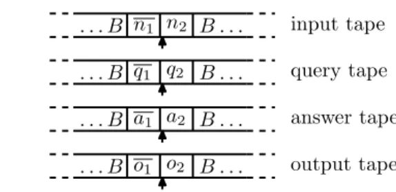
. . . B o1 o2 B . . . output tape . . . B a1 a2 B . . . answer tape . . . B q1 q2 B . . . query tape . . . B n1 n2 B . . . input tape
Figure 5: Encoding of the content of the tapes of an otm (or uotm). w represents the mirror of the word w and the arrows represent the positions of the heads.
Proof. Let f : (N −→ N)k −→ Nl−→ N be a function computed by a uotm M in time P , with P a second order polynomial. Without loss of generality, we will assume that k = l = 1. The idea of this proof is to write a program whose function symbol f0computes the output of M after t steps, and to use Lemma6to simulate the computation of P .
Let f0be the function symbol describing the execution of M: f0 :: [Bin] -> Nat -> Nat -> Bin8 -> Bin
The arguments of f0 represent respectively the input stream, the number of computational steps t, the current state and the 4 tapes (each tape is rep-resented by two binary numbers as illustrated in Figure 5). The output will correspond to the content of the output tape after t steps.
The function symbol f0 is defined recursively in its second argument: • if the timer is 0, then the program returns the content of the output tape
(after its head):
f0 s 0 q n1 n2 q1q2a1 a2o1 o2 = o2 • for each transition of M, we write a definition of this form:
f0 s (t+1) q n1 n2 q1 q2 a1 a2 o1 o2 = f0 s t q0 n01 n02 q 0 1 q02 a 0 1 a02 o 0 1 o02
where n1 and n2represent the input tape before the transition and n01and n02 represent the input tape after the transition, the motion and writing of the head being taken into account, and so on for the other tapes. Since the transition function is well described by a set of such definitions, the function f0produces the content of o2(i.e. the content of the output tape) after t steps on input t and configuration C (i.e. the state and the representations of the tapes).
f0 admits a polynomial interpretationLf0M. Indeed, in each definition, the state can only increase by a constant, the length of the numbers representing the various tapes cannot increase by more than 1. The answer tape La2M can undergo an important increase: when querying, it can increase by LsM(Lq2M), that is the interpretation of the input stream taken in the interpretation of the query.
Then we can provide a polynomial interpretation to f0: Lf0M(Y , T , Q, N1, N2, Q1, Q2, A1, A2, O1, O2) =
(T + 1) × (Y hQ2i + 1) + Q + N1+ N2+ Q1+ A1+ A2+ O1+ O2 Lemma 6 shows that the polynomial P can be implemented by a program p with a polynomial interpretation. Finally, consider the programs size, max, maxsize and f1 defined below:
size :: Bin -> Nat size Nil = 0
size (0 x) = (size x)+1 size (1 x) = (size x)+1 max :: Nat -> Nat -> Nat max 0 0 = 0
max 0 (k+1) = k+1 max (n+1) 0 = n+1
max (n+1) (k+1) = (max n k)+1 maxsize :: [Bin] -> Nat -> Nat maxsize (h:t) 0 = size h
maxsize (h:t) (n+1) = max (maxsize t n) (size h) f1 :: [Bin] -> Bin -> Bin
f1 s n = f0 s (p (maxsize s) (size n)) q0 Nil n Nil ... Nil
where q0is the index of the initial state, size computes the size of a binary number, and maxsize computes the size function of a stream of binary numbers. f1 computes an upper bound on the number of steps before M halts on input n with oracle s (i.e. P (|s|, |n|)), and simulates f0 within this time bound. The output is then the value computed by M on these inputs. Define the following polynomial interpretations for max, size and maxsize:
LsizeM(X ) = 2X
LmaxM(X1, X2) = X1+ X2 LmaxsizeM(Y , X ) = 2 × Y hX i
Finally f1 admits a polynomial interpretation since it is defined by compo-sition of programs with polynomial interpretations.
Adapting the proof of Lemma 7 in the case of an uotm without type-1 input (i.e. an ordinary Turing machine) allows us to state a similar result for type-1 functions (which can already be deduced from well known results in the literature).
Corollary 4. Every polynomial time computable type-1 function can be com-puted by a polynomial stream-free program.
5.2. Soundness
In order to prove the soundness result, we need to prove that the polynomial interpretation of a program can be computed in polynomial time by a uotm in this sense:
Lemma 8. If P is a second-order polynomial, then the function: F1, . . . , Fk, x1, . . . xl 7→ 2P (|F1|,...,|Fk|,|x1|,...,|xl|)− 1 is computable in polynomial time by a uotm.
Proof. The addition and multiplication on unary integers, and the function x 7→ |x| are clearly computable in polynomial time. Polynomial time is also stable under composition, so we only need to prove that the size function |F | is computable in polynomial time by a uotm. This is the case since it is a max over a polynomial number of elements of polynomial length. Note that this would not be true with the size function ||.|| as defined in [3] since is not computable in polynomial time.
Lemma 9 (Soundness). If a function symbol f :: [Bin]k -> Binl -> Bin admits a polynomial interpretation, then it computes a type-2 function f of type (N −→ N)k
−→ Nl
−→ N which is computable in polynomial time by a uotm. Proof. From the initial program (which uses streams), we can build a program using finite lists instead of streams as follows.
For each inductive type Tau, let us define the inductive type of finite lists over Tau:
data List(Tau) = Cons Tau List(Tau) | []
The type of each function symbol is changed from [Bin]k -> Binl -> Bin to List(Bin)k -> Binl -> Nat -> Bin (or from [Bin]k -> Binl -> [Bin] to List(Bin)k -> Binl -> Nat -> List(Bin)): streams are replaced by lists, and there is an extra unary argument. We also add an extra constructor Err to each type definition.
For each definition in the program, we replace the stream constructor (:) with the list constructor (Cons). We also add extra definitions matching the cases where some of the list arguments match the empty list ([]). In this case, the left part is set to Err. Whenever a function is applied to this special value, it returns it. This defines a new program with only inductive types, which behaves similarly to the original one.
app :: List(Bin) -> [Bin] app (Cons h t) = h : (app t) app [] = 0 : (app [])
It is easy to verify thatLappM(X)(Z) = X + 3Z is a correct interpretation. On strict values, the new program:
f’ v1 ... vk vk+1 vk+l
reduces as the original one with lists completed with app: f (app v1) ... (app vk) vk+1 vk+l.
The only differences are the additional reductions steps for app, but there is at most one additional reduction step for each stream argument each time there is a definition reduction ((d) rule in Figure4), so the total number of reductions is at most multiplied by a constant. The evaluation may also terminate earlier if the error value appears at some point.
The number of reduction steps is then bounded (up to a multiplicative con-stant) by:
LfM(Lapp v1M, . . . Lapp vkM, Lvk +1M, . . . Lvk +lM)
SinceLapp viM is a first order polynomial in the interpretation of vi, Lemma1 proves that the previous expression is a first order polynomial in the interpre-tation of its inputs. Several results in the literature (for example [21, 22]) on type-1 interpretations allow us to state that this new program computes a poly-nomial type-1 function (in particular because it is an orthogonal term rewriting system).
Let us now build a uotm which computes f. According to Lemma 8, given some inputs and oracles, we can computeLfM applied to their sizes and get a unary integer N in polynomial time. The uotm then computes the first N values of each type-1 input to obtain finite lists (of polynomial size) and then compute the corresponding list function on these inputs. According to Lemma5, since the input lists are long enough, the result computed by the list function and the stream function are the same.
5.3. Basic feasible functionals
In the completeness proof (Lemma 7), the program built from the uotm deals with streams using only the !! function to simulate oracle calls. This translation can be easily adapted to implement otms with stream programs. Because of the strict inclusion between polynomial time uotm computable func-tions and bff (cf. Lemma2) and the Lemma9, it will not always be possible to provide a polynomial interpretation to this translation, but a new proof provides us with a natural class of interpretation functions.
Definition 14 (exp-poly). Let exp-poly be the set of functions generated by the following grammar:
The interpretation of a program is exp-poly if each symbol is interpreted by an exp-poly function.
Example 10. P (Y, X) = Y h2X2+1i is in exp-poly, whereas 2X× Y h2Xi is not. Theorem 3. Every bff functional is computed by a program which admits an exp-poly interpretation.
Proof. Let f be a function computed by an otm M. We can reuse the con-struction from the proof of lemma7 to generate a function symbol f0(and its definitions) simulating the machine. Since we consider an otm and no longer a uotm, we should note that when querying, the query tape now contains a binary word, which we have to convert into unary before giving it to the !! function using an auxiliary function natofbin:
natofbin :: Bin -> Nat natofbin Nil = 0
natofbin (0 x) = plus (natofbin x) (natofbin x) natofbin (1 x) = (plus (natofbin x) (natofbin x)) +1
Its interpretation should verify, using the interpretation of plus given in Exam-ple6:
LnatofbinM(X + 1) > 3 × LnatofbinM(X ) + 1
This can be fulfilled with LnatofbinM(X ) = 22X. Note that this conversion function has no implementation with sub-exponential interpretation since the size of its output is exponential in the size of the input.
Now, in the new program, oracle calls are translated intos !! (natofbin a2), and the increase inLa2M is now bounded by LsM(2L2q2M).
We can define the interpretation of f0by:
Lf0M(Y , T , . . . , Q2, . . . ) = (T +1)×(Y h2
2Q2i+1)+Q+N
1+N2+Q1+A1+A2+O1+O2
Exp-poly functions are also computed by exp-poly programs using the same composition of natofbin and !!. Finally, the adaptation of the initial proof shows that f1will also have an exp-poly interpretation.
Remark 4. The soundness proof (Lemma9) does not adapt to bff and exp-poly programs, because the required analogue of Lemma8(where P is an exp-poly and the function is computable by a exp-polynomial time otm) is false (in particular, x, F 7→ 22F (x) is not basic feasible). Still, we conjecture that the converse of Theorem 3 holds. That is exp-poly programs only compute bff functionals.
6. Link with polynomial time computable real functions
Until now, we have considered stream programs as type-2 functionals in their own rights. However, type-2 functionals can be used to represent real functions. Indeed Recursive Analysis models computation on reals as computation on con-verging sequences of rational numbers [23, 17]. Note that there are numerous other possible applications, for example Kapoulas [24] uses uotm to study the complexity of p-adic functions and the following results could be adapted, since p-adic numbers can be seen as streams of integers between 1 ands p − 1.
We will require a given convergence speed to be able to compute effectively. A real x is represented by a sequence (qn)n∈N∈ QNif:
∀i ∈ N, |x − qi| < 2−i.
This will be denoted by (qn)n∈N x. In other words, after a query of size n, an uotm obtains an encoding of a rational number qn approaching its input with precision 2−n.
Definition 15 (Computable real function). A function f : R −→ R will be said to be computed by an uotm if:
(qn)n∈N x ⇒ (M(qn))n∈N f (x). (1) We will restrict to functions over the real interval [0, 1] (or any compact set). Hence a computable real function will be computed by programs of type [Q] -> [Q] in our stream language, where Q is an inductive type describing the set of rationals Q. For example, we can define the data type of rationals with a pair constructor /:
data Q = Bin / Bin
Only programs encoding machines verifying the implication (1) will make sense in this framework. Following [17], we can define polynomial complexity of real functions using polynomial time uotm computable functions.
The following theorems are applications of Theorem2 to this framework. Theorem 4 (Soundness). If a program f :: [Q] -> [Q] with a polynomial interpretation computes a real function, then this function is computable in poly-nomial time.
Proof. Let us define g from f :: [Q] -> [Q]: g :: [Q] -> Nat -> Q
g s n = (f s) !! n
If f has a polynomial interpretationLfM, then g admits the polynomial inter-pretationLgM(Y, N) = LfM(Y, N) + 1 (using the usual interpretation of !! defined in Example8).
The type of rational numbers can be seen as pairs of binary numbers, so Theorem2can be easily adapted to this framework. A machine computes a real function in polynomial time if and only if it outputs the nthelement of the result
in polynomial with respect to the size of the input (as defined in Definition4) and n. In this sense, the machine constructed from g using Theorem2computes the real function computed by f.
Example 11. The square function over the real interval [0, 1] can be imple-mented in our stream language, provided we already have a function symbol bsqr :: Bin -> Bin implementing the square function over binary integers: Rsqr :: [Q] -> [Q]
Rsqr (h : t) = Ssqr t Ssqr :: [Q] -> [Q]
Ssqr ((a / b) : t) = (bsqr a / bsqr b) : (Ssqr t)
Ssqr squares each element of its input stream. Rsqr removes the head of its input before applying Ssqr because the square function requires one additional precision unit on its input:
∀n ∈ N, |qn− x| ≤ 2−n⇒ ∀n ∈ N, |qn+12 − x2| ≤ 2−n
This allows us to prove that the output stream converges at the right speed and that Rsqr indeed computes the real square function on [0, 1]. Now, set the polynomial interpretations:
LSsqrM(Y, Z) = 2 × Z × LbsqrM(YhZi)
LRsqrM(Y, Z) = 2 × Z × LbsqrM(YhZ + 1i) They are indeed valid:
LSsqr ((a / b) : t)M(Z + 1) = 2(Z + 1)LbsqrM(2 + A + B + T(Z)) > 2 +LbsqrM(A) + LbsqrM(B) + 2ZLbsqrM(T(Z − 1)) =L(bsqr a / bsqr b) : (Ssqr t)M and LRsqr (h : t)M(Z) = 2Z LbsqrM(1 + H + T(Z − 1 + 1) > 2ZLbsqrM(T(Z)) = LSsqr tM
Theorem 5 (Completeness). Any polynomial-time computable real function can be implemented by a polynomial program.
Proof. Following [17], we can describe any computable real function f by two functions fQ : N × Q −→ Q and fm : N −→ N where fQ(n, q) computes an approximation of f (q) with precision 2−n:
∀q, (fQ(n, q))n∈N f (q) and fmis a modulus of continuity of f defined as follows:
For a polynomial-time computable real function, those fm and fQ are discrete functions computable in polynomial time. Corollary4 ensures that these func-tions can be implemented by programs fQ and fm with polynomial interpreta-tions. Then, we can easily derive a program that computes f by first finding which precision on the input is needed (using fm) and computing with fQ an approximation of the image of the input.
faux :: Nat -> [Q] -> [Q]
faux n y = (fQ n (y !! (fm n))) : (faux (n+1) y) f :: [Q] -> [Q]
f y = faux 0 y
with Q an inductive type representing rational numbers. We can easily check that these interpretations work:
LfauxM(Y, N, Z) = (Z + 1) × (1 + LfQM(N + Z, YhLfmM(N + Z)i))
LfM(Y, Z) = 1 + LfauxM(Y, 1, Z)
7. Conclusion
We have provided a characterization of polynomial time stream complexity using basic polynomial interpretations and this the first characterization of this kind. More complex and finer interpretation techniques on first order complex-ity classes (e.g. sup-interpretations or quasi-interpretations) could probably be adapted to stream languages.
This work also provides a partial characterization of bff and shows that it is not the right feasible complexity class for functions over streams. Our framework also adapts well to applications like computable analysis. We have indeed characterized the class of polynomial time real functions, and this is again the first time that this class is characterized using interpretations.
As a whole, this work is a first step toward higher order complexity. We have used second order interpretations, but higher order interpretations could also be used to characterize higher order complexity classes. The main difficulty is that the state of the art on higher order complexity rarely deal with orders higher than two.
References
[1] R. L. Constable, Type two computational complexity, in: Proc. 5th annual ACM STOC, 108–121, 1973.
[2] K. Mehlhorn, Polynomial and abstract subrecursive classes, in: Proceedings of the sixth annual ACM symposium on Theory of computing, ACM New York, NY, USA, 96–109, 1974.
[3] B. M. Kapron, S. A. Cook, A new characterization of type-2 feasibility, SIAM Journal on Computing 25 (1) (1996) 117–132.
[4] A. Seth, Turing machine characterizations of feasible functionals of all finite types, Feasible Mathematics II (1995) 407–428.
[5] R. J. Irwin, J. S. Royer, B. M. Kapron, On characterizations of the basic feasible functionals (Part I), J. Funct. Program. 11 (1) (2001) 117–153. [6] R. Ramyaa, D. Leivant, Ramified Corecurrence and Logspace, Electronic
Notes in Theoretical Computer Science 276 (0) (2011) 247 – 261, ISSN 1571-0661.
[7] R. Ramyaa, D. Leivant, Feasible Functions over Co-inductive Data, in: Logic, Language, Information and Computation, vol. 6188 of Lecture Notes in Computer Science, Springer Berlin / Heidelberg, ISBN 978-3-642-13823-2, 191–203, 2010.
[8] S. Bellantoni, S. A. Cook, A New Recursion-Theoretic Characterization of the Polytime Functions, Computational Complexity 2 (1992) 97–110. [9] D. Leivant, J.-Y. Marion, Lambda Calculus Characterizations of
Poly-Time, Fundam. Inform. 19 (1/2) (1993) 167–184.
[10] G. Bonfante, J.-Y. Marion, J.-Y. Moyen, Quasi-interpretations a way to control resources, Theoretical Computer Science 412 (25) (2011) 2776 – 2796, ISSN 0304-3975.
[11] P. Baillot, U. D. Lago, Higher-Order Interpretations and Program Com-plexity, in: P. C´egielski, A. Durand (Eds.), CSL, vol. 16 of LIPIcs, Schloss Dagstuhl - Leibniz-Zentrum fuer Informatik, ISBN 978-3-939897-42-2, 62– 76, 2012.
[12] Z. Manna, S. Ness, On the termination of Markov algorithms, in: Third Hawaii international conference on system science, 789–792, 1970.
[13] D. Lankford, On proving term rewriting systems are Noetherian, Tech. Rep., Mathematical Department, Louisiana Technical University, Ruston, Louisiana, 1979.
[14] J.-Y. Marion, R. P´echoux, Sup-interpretations, a semantic method for static analysis of program resources, ACM Trans. Comput. Logic 10 (4) (2009) 27:1–27:31, ISSN 1529-3785.
[15] M. Gaboardi, R. P´echoux, Upper Bounds on Stream I/O Using Semantic Interpretations, in: E. Gr¨adel, R. Kahle (Eds.), CSL, vol. 5771 of Lecture Notes in Computer Science, Springer, ISBN 978-3-642-04026-9, 271–286, 2009.
[17] K.-I. Ko, Complexity theory of real functions, Birkhauser Boston Inc. Cam-bridge, MA, USA, 1991.
[18] H. F´er´ee, E. Hainry, M. Hoyrup, R. P´echoux, Interpretation of Stream Programs: Characterizing Type 2 Polynomial Time Complexity, in: Algo-rithms and Computation, vol. 6506 of Lecture Notes in Computer Science, Springer Berlin / Heidelberg, ISBN 978-3-642-17516-9, 291–303, 2010. [19] R. P´echoux, Synthesis of sup-interpretations: A survey, Theor. Comput.
Sci. 467 (2013) 30–52.
[20] J. Endrullis, C. Grabmayer, D. Hendriks, A. Isihara, J. W. Klop, Produc-tivity of stream definitions, Theor. Comput. Sci. 411 (4-5) (2010) 765–782. [21] G. Bonfante, A. Cichon, J.-Y. Marion, H. Touzet, Algorithms with polyno-mial interpretation termination proof, Journal of Functional Programming 11 (01) (2001) 33–53.
[22] U. Lago, S. Martini, Derivational Complexity Is an Invariant Cost Model, in: M. Eekelen, O. Shkaravska (Eds.), Foundational and Practical Aspects of Resource Analysis, vol. 6324 of Lecture Notes in Computer Science, Springer Berlin Heidelberg, ISBN 978-3-642-15330-3, 100–113, 2010. [23] K. Weihrauch, Computable analysis: an introduction, Springer Verlag,
2000.
[24] G. Kapoulas, Polynomially Time Computable Functions over p-Adic Fields, in: J. Blanck, V. Brattka, P. Hertling (Eds.), Computability and Complex-ity in Analysis, vol. 2064 of Lecture Notes in Computer Science, Springer Berlin Heidelberg, ISBN 978-3-540-42197-9, 101–118, 2001.