HAL Id: hal-01695076
https://hal.univ-reims.fr/hal-01695076
Submitted on 15 Feb 2018
HAL is a multi-disciplinary open access
archive for the deposit and dissemination of
sci-entific research documents, whether they are
pub-lished or not. The documents may come from
teaching and research institutions in France or
abroad, or from public or private research centers.
L’archive ouverte pluridisciplinaire HAL, est
destinée au dépôt et à la diffusion de documents
scientifiques de niveau recherche, publiés ou non,
émanant des établissements d’enseignement et de
recherche français ou étrangers, des laboratoires
publics ou privés.
Implicit component-graph: A discussion
Nicolas Passat, Benoît Naegel, Camille Kurtz
To cite this version:
Nicolas Passat, Benoît Naegel, Camille Kurtz. Implicit component-graph: A discussion.
Interna-tional Symposium on Mathematical Morphology (ISMM), 2017, Fontainebleau, France. pp.235-248,
�10.1007/978-3-319-57240-6_19�. �hal-01695076�
Nicolas Passat1, Benoˆıt Naegel2, and Camille Kurtz3
1Universit´e de Reims Champagne-Ardenne, CReSTIC, France
2Universit´e de Strasbourg, CNRS, ICube, France
3Universit´e Paris-Descartes, LIPADE, France
Abstract. Component-graphs are defined as the generalization of component-trees to images taking their values in partially ordered sets. Similarly to compo-nent-trees, component-graphs are a lossless image model, and can allow for the development of various image processing approaches (e.g., antiextensive filter-ing, segmentation by node selection). However, component-graphs are not trees, but directed acyclic graphs. This induces a structural complexity associated to a higher combinatorial cost. These properties make the handling of component-graphs a non-trivial task. We propose a preliminary discussion on a new way of building and manipulating component-graphs, with the purpose of reaching reasonable space and time costs. Tackling these complexity issues is indeed re-quired for actually involving component-graphs in efficient image processing ap-proaches.
Keywords: component-graph, algorithmics, data-structure.
1
Introduction
In mathematical morphology, connected operators [1] are often defined from hierarchi-cal image models, namely trees, that represent an image by considering simultaneously its spatial and spectral properties. Among the most popular tree structures modelling images, one can cite the component-tree (CT) [2], the tree of shapes (ToS) [3], and the binary partition tree (BPT) [4]. The CT and ToS —by contrast with the BPT, that de-rives from both an image and extrinsic criteria— are intrinsic models, that depend only on the image pixel values, and are built in a deterministic way.
Initially, the CT and the ToS (which can be seen as an autodual version of the CT) were defined for grey-level images, i.e. images whose values are totally ordered. Di ffer-ent ways to extend the notions of CT and ToS to multivalued images, i.e. images whose values are partially ordered, were investigated during the last years. The purpose was, in particular, to allow for the use of such image models in a wider range of image process-ing applications. The first attempt of extendprocess-ing the notion of CT to partially-ordered values was proposed in [5], leading to the pioneering notion of component-graph (CG). The main structural properties of CGs were further established [6]. From an algorithmic point of view, first strategies for building CGs were investigated. Except in a specific case —where the partially ordered set of values is structured itself as a tree [7]— these first attempts emphasised the high computational cost of the construction process, and the high spatial cost of the directed acyclic graph (DAG) explicitly modelling a CG [8,
9]. By relaxing certain constraints, leading to an improved complexity, the notion of CG was successfully involved in the development of an efficient extension of ToS to multivalued images [10]. From an applicative point of view, the notion of CG, coupled with the recent notion of shaping [11], also led to preliminary, yet promising, results for multimodal image processing [12].
In this paper, we propose a preliminary discussion on a new way of building and manipulating CGs. A CG is complex due to its size (i.e. its number of nodes and edges) and its structural complexity (as a DAG), which both induce high space and time com-putational costs. Our strategy is to take advantage of the structural properties of a CG in order to build dedicated data-structures gathering information useful for handling it, without explicitly computing its whole DAG. We then hope to obtain a reasonable trade-off between the cost of modelling the CG, and the cost of navigating within it for further image processing purposes.
The following discussion is mainly theoretical, providing preliminary ideas; in par-ticular, we will present neither experimental studies nor application cases. The remain-der of the paper is organized as follows. Sections 2 and 3 provide notations and re-call basic notions on CGs. In Section 4, we enumerate the different functionalities that should be offered by implicit CG data-structures. Sections 5–11 constitute the core of the paper, where we develop our discussion. Section 12 provides concluding remarks.
2
Notations
The used notations are the same as in [6–9]. We only recall here the non-standard ones. For any symbol further used to denote an order relation (⊆,6, E, etc.), the inverse symbol (⊇,>, D, etc.) denotes the associated dual order, while the symbol without lower bar (⊂, <,C, etc.) denotes the associated strict order.
If (X,6) is an ordered set and x ∈ X, we note x↑ = {y ∈ X | y > x} and x↓ = {y ∈ X | y6 x}, namely the sets of the elements greater and lower than x, respectively. If Y ⊆ X, the sets of all the maximal and minimal elements of Y are noted`6Yanda6Y, respectively.
3
Basic Notions on Component-Graphs
Let Ω be a nonempty finite set. Let V be a nonempty finite set equipped with an or-der (i.e. reflexive, transitive, antisymmetric) relation6. We assume that (V, 6) admits a minimum, noted ⊥.
We call an image any function I: Ω −→ V x 7−→ v (1)
Without loss of generality, we assume that I−1({⊥})= {x ∈ Ω | I(x) = ⊥} , ∅. For any v ∈ V, the thresholding function at value v is defined by
λv: VΩ−→ 2Ω I 7−→ {x ∈Ω | v 6 I(x)} (2)
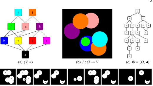
a d b c e f g h j i (a) (V, ≺) (b) I : Ω → V A G H C B D E F S Q R I J K M N O L P (c) G= (Θ, J) B F (d) λb(I) D E C (e) λc(I) G M (f) λd(I) H N (g) λe(I) I O X X (h) λf(I) J K (i) λg(I) Q L (j) λh(I) R X X (k) λi(I) P S (l) λj(I)
Fig. 1. (a) The Hasse diagram (V, ≺) of an ordered set (V,6), with V = {a, b, c, d, e, f, g, h, i, j} (for the sake of readability, each value of V is associated to an arbitrary colour). (b) An image
I : Ω → V. (c) The component-graph G of I. (d–l) Thresholded images λv(I) for v ∈ V (the
threshold image λa(I) is not depicted: it is composed of an unique connected component A equal
to Ω). The letters (A–S) in nodes (c) correspond to the associated connected components in (d–l).
Leta be an adjacency (i.e. irreflexive, symmetric) relation on Ω (the restriction of a to any subset of Ω is also noteda). For any X ⊆ Ω, the set of the connected components of the graph (X,a), i.e. the equivalence classes of X with respect to the connectedness relation (i.e. the reflexive–transitive closure) induced bya, is noted C[X]. Without loss of generality, we assume that (Ω,a) is connected, i.e. C[Ω] = {Ω}.
Definition 1 (Valued connected component) Let v ∈ V and X ∈ C[λv(I)]. The couple K= (X, v) is called a valued connected component; X is the support of K while v is its value. We define the set Θ of all the valued connected components of I as
Θ =[ v∈V
C[λv(I)] × {v} (3)
From the order relation6 on V, and the inclusion relation ⊆ on 2Ω(the power-set of Ω), we define the order E on Θ as
(X1, v1)E (X2, v2) ⇐⇒ (X1⊂ X2) ∨ (X1= X2∧ v2 6 v1) (4) In other words, we enrich the standard inclusion relation, by considering the order on V whenever two valued connected components have the same support. We noteJ the cover relation associated toE, i.e. for all K1 , K2 ∈Θ, we have K1 J K2iff K1 E K2 and there is no K3∈Θ distinct from K1, K2such that K1E K3 E K2.
Definition 2 (Component-graph [5, 6]) TheΘ-component-graph (or simply, the com-ponent-graph) of I is the Hasse diagram G = (Θ, J) of the ordered set (Θ, E). The elements ofΘ are called nodes; the elements of J are called edges; (Ω, ⊥) is called the root; the elements ofaEΘ are called the leaves of the component-graph.
The component-graph G of I is then the Hasse diagram of the ordered set (Θ,E) (see Figure 1, for an example). Two other (simpler) variants1of CGs were also proposed in [6]. They will not be considered in this study for the sake of concision.
4
Problem Statement
Let I : Ω → V be an image defined on a set Ω endowed with an adjacencya, and taking its values in a set V equipped with an order6. Our purpose is to build dedicated data-structures that model the component-graph G of I without explicitly building its whole DAG, and to be able to use them in an efficient way for further image processing purposes. In particular, the main questions that should be easily answered thanks to such data-structures are the following:
(i) Who are the nodes of G (i.e. how to identify them)? (ii) What is a node of G (i.e. what are its support and its value)?
(iii) Is a node of G lower, greater, or non-comparable to another, with respect toE? The following sections aim at discussing about the construction of ad hoc data-struc-tures that could allow for answering these questions.
5
Flat Zones and Leaves
5.1 Flat Zone Image
Let x, y ∈ Ω be two points of the image I. If x and y are adjacent, i.e. xa y, and share the same value, i.e. I(x)= I(y), then it is plain that they belong the same valued connected components of G, i.e. for any K = (X, v) ∈ Θ, we have x ∈ X iff y ∈ X. As an immediate corollary, the component-graph obtained from I is isomorphic to the component-graph of the flat zone image2associated to I.
A linear time cost O(|a|) flat zone computation can then allow us to simplify the image I into its flat zone analogue, thus reducing the space complexity of the image. From now on, and without loss of generality, we will work on such flat zone images, still noted I : Ω → V for the sake of readability, and since they are indeed equivalent for CG building. In particular, under this hypothesis, we have the following property. Property 3 Let x, y ∈ Ω. If x and y are adjacent, then their values are distinct, i.e. xa y ⇒ I(x) , I(y).
1These two variants, called ˙Θ- and ¨Θ-component-graphs, rely on sets of nodes defined as subsets
of Θ. A ¨Θ-component graph only contains nodes that are necessary to model I in a lossless
way, while the ˙Θ-component-graph contains nodes with maximal values for a given support.
2The image where each flat zone (i.e. maximal connected region of constant value) is replaced
by a single point, and where the adjacency relation between these flat zones is inherited froma (i.e. two flat zones are adjacent iff one point of the first is adjacent to one point of the second).
5.2 Detection of the Leaves
Since Ω is finite and6 is antisymmetric, there exist n ≥ 1 points x ∈ Ω such that for all ya x, we have I(x) ≮ I(y), i.e. I(x) ∈ V is a locally maximal value of the image I. Then, it is plain that Kx= ({x}, I(x)) is a node of G, i.e. Kx ∈Θ. More precisely, Kxis a minimal element of G, i.e. Kx∈aEΘ, and is then a leaf of G (see Definition 2). As an example, the leaves of the component-graph G depicted on Figure 1(c) correspond to the nodes I, S, R, and P.
The characterization of the leaves relying on a local criterion, we can then detect all of them by an exhaustive scanning of Ω, with a linear time cost3 O(|a|). In the sequel, we will denote by Λ ⊆ Ω the set of all the points of Ω that correspond to supports of leaves. In other words, we haveaEΘ = {Kx= ({x}, I(x)) | x ∈ Λ}.
6
Node Encoding
Let K = (X, v) ∈ Θ be a node of G. If K is not a leaf, i.e. K < aEΘ, then there exists a leaf Kx = ({x}, I(x)) ∈ aEΘ such that Kx E K. In particular, Equation (4) implies that x ∈ X and I(x) > v. In [6, Property 1], we observed that for a given leaf Kx = ({x}, I(x)) ∈ aEΘ, and for any value v 6 I(x), there exists exactly one node K= (X, v) ∈ Θ such that x ∈ X.
This allows us to define the function4 κ : Λ × V −→ Θ ∪ {K>} (x, v) 7−→ K= (X, v) ∈ Θ s.t. x ∈ X if v 6 I(x) (x, v) 7−→ K> otherwise (5)
This function encodes each node (X, v) ∈ Θ of G based on two kinds of information: (1) the value v of the node, and (2) a point x ∈ Λ ∩ X of locally maximal value, lying within the support of the node.
The function κ is obviously surjective5: each node K= (X, v) ∈ Θ corresponds to a couple (x, v) ∈ Λ × V such that κ((x, v))= K. This justifies the following property. Property 4 The setΘ of the nodes of G is defined as Θ = κ(Λ × V) \ {K>}.
However, κ is generally not injective. It is then necessary to handle the synonymy of nodes with respect to κ.
3In digital imaging, we have |a| = O(|Ω|) (e.g. with 4-, 8-, 6- and 26-adjacencies on Z2and Z3,
we have |a| ' k.|Ω|, with k = 2, 4, 3 and 13, respectively), and this generally still holds for the induced flat zone images. Under such hypotheses, the detection of leaves can be performed in linear time O(|Ω|) with respect to the size of the image. For the sake of concision, we will assume, from now on, that we have indeed |a| = O(|Ω|).
4By convention, we define a supplementary node K
>for handling the cases when the considered
value v is greater than (or non-comparable with) the value I(x) associated to x, in order to define κ on the whole Cartesian set Λ × V. This does not induce any algorithmic nor structural issue.
5Actually, it is surjective iff κ−1({K
>}) , ∅. If κ−1({K>})= ∅, we can simply define κ : Λ × V →
7
Node Synonymy Handling
Let K1 = (X1, v1), K2 = (X2, v2) ∈ Θ be nodes of G. From Property 4, there exist x1, x2 ∈ Λ such that κ((x1, v1)) = K1 and κ((x2, v2)) = K2. If v1 , v2, it is plain that K1 , K2. However, when v1 = v2, we may have x1, x2while K1= K2, i.e. X1= X2.
In other words, a node K = (X, v) ∈ Θ —and more precisely its support X— can be represented by any point x ∈ Λ ∩ X, that also corresponds to the support of a leaf Kx= ({x}, I(x)) ∈ aEΘ. In order to provide an actual modelling of the nodes of G from κ, we then have to gather the elements of Λ × V that encode a same node.
To this end, we define the equivalence relation ∼ on Λ × V as (x1, v1) ∼ (x2, v2) ⇔ κ((x1, v1))= κ((x2, v2)). From this relation and the function κ, we derive a new function
κ∼: (Λ × V)/∼ −→ Θ ∪ {K>} [(x, v)]∼ 7−→κ((x, v)) (6) that inherits the surjectivity of κ while guaranteeing, by construction, injectivity. In order to obtain a modelling of the set of nodes Θ of G based on a Λ × V encoding, it is then sufficient to compute the equivalence classes induced by the relation ∼.
It is plain that for any (x, v) ∈ Λ × V, the equivalence class [(x, v)]∼is composed of elements (x0, v) with different x0∈Λ, but a same value v. Then, it is possible to partition the set of equivalence classes of ∼ with respect to the different values of V. Indeed, for any v ∈ V, we can define the equivalence relation ∼von Λ as x1 ∼v x2 ⇔κ((x1, v)) = κ((x2, v)). In particular, we have [(x, v)]∼= [x]∼v× {v}.
Another important property is the increasingness of these equivalence classes with respect to the decreasingness of6, that is the fact that for any x ∈ Λ, we have v16 v2⇒ [x]∼v2 ⊆ [x]∼v1. This property can also be written as
v16 v2=⇒ ((x ∼v2y) ⇒ (x ∼v1 y)) (7)
then justifying the following property.
Property 5 The characterization of ∼ only requires to define, for each v ∈ V, the rela-tions x ∼vy such that for ∀v0> v, x v0y.
Practically, this property states that the issue of synonymy between nodes could take advantage of the monotony of ∼v (v ∈ V) with respect to6, to avoid the storage of information already carried by the structure of (V,6) (see Section 12).
The next step is now to define a way to actually build these equivalence classes.
8
Reachable Zones
In order to build the equivalence relation ∼, let us come back to the image I and its adjacency graph (Ω,a). Each point x ∈ Ω has a given value I(x) ∈ V. It is also adjacent to other points y ∈ Ω (i.e. x a y) with values I(y). From Property 3, we have either I(x) < I(y) or I(x) > I(y) or I(x), I(y) non-comparable.
From a point x ∈ Λ, we can reach certain points y ∈ Ω by a descent paradigm. More precisely, for such points y, there exists a path x= x0 a . . . a xia . . . a xt= y (t ≥ 0) in Ω such that for any i ∈ [[0, t − 1]], we have I(xi) > I(xi+1). In such case, we note x & y. This leads to the following notion of a reachable zone.
Definition 6 (Reachable zone) Let x ∈ Λ. The reachable zone of x (in I) is the set ρ(x) = {y ∈ Ω | x & y}.
When a point y ∈ Ω belongs to the reachable zone ρ(x) of a point x ∈ Λ, the adjacency path from x to y and the > relation between its successive points imply that the node (Y, I(y)) ∈ Θ with y ∈ Y satisfies x ∈ Y. This justifies the following property.
Property 7 Let x ∈Λ. Let v ∈ V such that v 6 I(x). Let K = κ((x, v)) = (X, v) ∈ Θ. We have
{y ∈ρ(x) | v 6 I(y)} ⊆ X (8) This property states that the supports of the nodes K= (X, v) ∈ Θ of G can be partially computedfrom the reachable zones of the points of Λ. These computed supports may be yet incomplete, since X can lie within the reachable zones of several points of Λ within a same equivalence class [x]∼v.
However, the following property, that derives from Definition 6, guarantees that no point of Ω will be omitted when computing the nodes of Θ from unions of reachable zones.
Property 8 The set {ρ(x) | x ∈ Λ} is a cover of Ω. The important fact of this property is thatS
x∈Λρ(x) = Ω. However, the set of reachable zones is not a partition of Ω, in general, due to possible overlaps. For instance, let x1, x2 ∈Λ, y ∈ Ω, and let us suppose that x1 a y a x2and x1 > y < x2; then we have y ∈ρ(x1) ∩ ρ(x2) , ∅.
Remark 9 The computation of the reachable zones can be carried out by a seeded region-growing, by considering Λ as set of seeds. The time cost is output-dependent, since it is linear with respect to the ratio of overlap between the different reachable zones. More precisely, it is O(P
x∈Λ|ρ(x)|) = O((1 + γ).|Ω|), with γ ∈ [0, |Ω|/4] ⊂ R the overlap ratio6, varying between0 (no overlap between reachable zones, i.e. {ρ(x) | x ∈ Λ} is a partition of Ω) and |Ω|/4 (all reachable zones are maximally overlapped).
The fact that two reachable zones may be adjacent and/ or overlap will allow us to complete the construction of the nodes K ∈ Θ of G.
9
Reachable Zone Graph
9.1 Reachable Zone Adjacency
When two reachable zones are adjacent —a fortiori when they overlap— they contribute to the definition of common supports for nodes of the component-graph.
Let x1, x2 ∈Λ (x1, x2), and let us consider their reachable zones ρ(x1) and ρ(x2). Let y1 ∈ρ(x1) and y2 ∈ρ(x2) be two points such that y1 a y2. Let us consider a value v ∈ V such that v 6 I(y1) and v 6 I(y2). Since we have y1 a y2, and from the very definition of reachable zones (Definition 6), there exists a path x1 = z0 a . . . a zi a . . . a zt = x2 (t ≥ 1) within ρ(x1) ∪ ρ(x2) such that v 6 I(zi) for any i ∈ [[0, t]]. This justifies the following property.
Property 10 Let x1, x2 ∈Λ with x1, x2. Let us suppose that there exists y1 a y2with y1 ∈ ρ(x1) and y2 ∈ ρ(x2). Then, for any v ∈ V such that v6 I(y1) and v6 I(y2), we haveκ((x1, v)) = κ((x2, v)), i.e. (x1, v) ∼ (x2, v), i.e. x1∼vx2.
This property provides a way to build the equivalence classes of ∼v (v ∈ V) and then ∼. In particular, we can derive a notion of adjacency between the points of Λ or, equivalently, between their reachable zones, leading to a notion of reachable zone graph.
Definition 11 (Reachable zone graph) Let aΛ be the adjacency relation defined on Λ ⊆ Ω as
x1aΛx2⇐⇒ ∃(y1, y2) ∈ ρ(x1) × ρ(x2), y1 a y2 (9) The graph R= (Λ, aΛ) is called reachable zone graph (of I).
9.2 Reachable Zone Graph Valuation
The structural description provided by the reachable zone graph R of I is necessary, but not sufficient for building the equivalence classes of ∼, and then actually building the nodes of the component-graph G via the function κ. Indeed, as stated in Property 10, we also need information about the values of V associated to the adjacency links. This leads us to define a notion of valuation onaLor, more generally7, on Λ × Λ.
Definition 12 (Valued reachable zone graph) Let R= (Λ, aΛ) be the reachable zone graph of an image I: Ω → V. We define the valuation function σ on the edges of R as
σ : Λ × Λ −→ 2V
(x1, x2) 7−→ {v | ∃(y1, y2) ∈ ρ(x1) × ρ(x2), y1a y2∧ I(y1)> v 6 I(y2)} if x1aΛx2
(x1, x2) 7−→ ∅ if x16aΛx2
(10) The couple(R, σ) is called valued reachable zone graph (of I).
Remark 13 For any x1, x2 ∈Λ, we have σ((x1, x1))= ∅ and σ((x1, x2))= σ((x2, x1)). Actually, the definition of σ only requires to consider the couples of points located at the bordersof reachable zones, as stated by the following reasoning. Let x1, x2 ∈Λ (x1, x2). Let v ∈ σ((x1, x2)). Then, there exist y1 ∈ρ(x1) and y2 ∈ρ(x2) with y1a y2, such that I(y1) > v 6 I(y2). Now, let us assume that we also have y1 ∈ρ(x2) and y2 ∈ ρ(x1), i.e. y1, y2∈ρ(x1) ∩ ρ(x2). There exists a path x1 = z0 a . . . a zia . . . a zt = y1 (t ≥ 1) within ρ(x1), with I(zi) > I(zi+1) for any i ∈ [[0, t − 1]]. Let j= max{i ∈ [[0, t]] | zi < ρ(x2)} (we necessarily have j < t). Let v0 = I(zj+1). By construction, we have (zj, zj+1) ∈ ρ(x1) × ρ(x2), zj a zj+1and I(zj) > v0 > v 6 v0 6 I(zj+1). Then v could be characterized by considering a couple of points (zj, zj+1) with zj ∈ρ(x1) \ ρ(x2) and zj+1∈ρ(x2), i.e. with zj+1at the border of ρ(x2). This justifies the following property.
7The adjacency relation
aL is indeed a subset of the Cartesian product Λ × Λ; so it would
be sufficient to define the function σ : aL → 2V. However, such notation is unusual and
probably confusing for many readers; then, we prefer to define, without loss of correctness, σ : Λ × Λ → 2V, with useless empty values for the couples (x
Property 14 Let x1, x2 ∈ Λ. Let v ∈ V. We have v ∈ σ((x1, x2)) iff there exists y1 ∈ ρ(x1) \ ρ(x2) and y2∈ρ(x2) such that y1a y2and I(y1)> v 6 I(y2).
Based on this property, the construction of the sets of values σ((x1, x2)) ∈ 2V for each couple (x1, x2) ∈ Λ × Λ can be performed by considering only a reduced subset of edges ofa, namely the couples y1 a y2such that y1 ∈ρ(x1) \ ρ(x2) and y2 ∈ρ(x2), i.e. the border of the reachable zone of x2 adjacent to/ within the reachable zone of x1. In particular, these specific edges can be identified during the computation of the reachable zones, without increasing the time complexity of this step.
Now, let us focus on the determination of the values v ∈ V to be stored in σ((x1, x2)), when identifying a couple y1 a y2such that y1∈ρ(x1)\ρ(x2) and y2∈ρ(x2). Practically, two cases, can occur. Case 1: I(y1) > I(y2), i.e. y2∈ρ(x1) ∩ ρ(x2). Then all the values v6 I(y2) are such that I(y1)> v 6 I(y2); in other words, we have I(y2)↓ ⊆σ((x1, x2)). Case 2: I(y2) and I(y1) are non-comparable, i.e. y2∈ρ(x2) \ ρ(x1). Then, the values that belong to σ((x1, x2)) with respect to this specific edge are those simultaneously below I(y1) and I(y2); in other words, we have (I(y1)↓∩ I(y2)↓) ⊆ σ((x1, x2)).
Remark 15 Instead of exhaustively computing the whole set of valuesσ((x1, x2)) ∈ 2V associated to the edge x1aΛ x2, it is sufficient to determine the maximal values of such a subset of V. We can then consider the functionσO : Λ × Λ → 2V, associated toσ, and defined byσO((x1, x2)) = `6σ((x1, x2)). In particular for any x1 aΛ x2, we have v ∈σ((x1, x2)) iff there exists v0∈σO((x1, x2)) such that v6 v0.
10
Algorithmic Sketch
Based on the above discussion, we now recall the main steps of the algorithmic process for the construction of data-structures allowing us to handle a component-graph.
10.1 Input/ Output
The input of the algorithm is an image I, i.e. a function I : Ω → V, defined on a graph (Ω,a) and taking its values in an ordered set (V, 6). Note that I is first preprocessed in order to obtain a flat zone image (see Section 5.1); this step presents no algorithmic dif-ficulty and allows for reducing the space cost of the image without altering the structure of the component-graph to be further built.
The output of the algorithm, i.e. the set of data-structures required to manipulate the component-graph implicitly modelled, is basically composed of:
– the ordered set (V,6) (and / or its Hasse diagram (V, ≺)); – the initial graph (Ω,a), equipped with the function I : Ω → V; – the set of leaves Λ ⊆ Ω;
– the function ρ : Λ → 2Ω that maps each leaf to its reachable zone (and/ or its “inverse” function ρ−1 : Ω → 2Λthat indicates, for each point of Ω, the reachable zone(s) where it lies);
– the reachable zone graph R= (Λ, aΛ);
– the valuation function σ : Λ × Λ → 2V (practically, σ :aΛ→ 2V) or its “compact” version σO.
10.2 Algorithmics and Complexity
The initial graph (Ω,a) and the ordered set (V, 6) are provided as input. The space cost of (Ω,a) is O(|Ω|) (we assume that |a| = O(|Ω|)). The space cost of (V, 6) is O(|V|) (by modelling6 via its Hasse diagram, i.e. its transitive reduction, we can assume that |6| = O(|V|)). The space cost of I is O(|Ω|).
As stated in Section 5.2, the set of leaves Λ ⊆ Ω is computed by a simple scanning of Ω, with respect to the image I. This process has a time cost O(|Ω|). The space cost of Λ is O(|Ω|) (with, in general, |Λ| |Ω|).
As stated in Section 8, the function ρ (and equivalently, ρ−1) is computed by a seeded region-growing. This process has a time cost which is output-dependent, and in particular equal to the space cost of the output; this cost is O(|Ω|α) with α ∈ [1, 2]. One may expect that, for standard images, we have α ' 1.
The adjacencyaΛcan be computed on the fly, during the construction of the reach-able zones. By assuming that, at a given time, the reachreach-able zones of Λ+ are already constructed while those of Λ−are not yet (Λ+∪Λ−= Λ), when building the reachable zone of x ∈ Λ−, if a point y ∈ Ω is added to ρ(x), we add the couple (x, x0) toaΛif there exists z ∈ ρ(x0) in the neighbourhood of y, i.e. za y. This process induces no extra time cost to that of the above seeded region-growing. The space cost ofaΛis O(|Λ|β) with β ∈ [1, 2]. One may expect that, for standard images, we have β ' 1.
The valuation function σ : Λ × Λ → 2V is built by scanning the adjacency links ofa located on the borders of the reachable zones8. This subset of adjacency links has a space cost O(|Ω|δ), with δ ∈ (0, 1]. One may expect that δ 1, due to the fact that we consider borders of regions9. For each adjacency link of this subset ofa, one or several values (their number can be expected to be, in average, a low constant value k) are stored in σ. This whole storage then has a time cost O(k.|Ω|δ). Then, some of these values are removed, since they do not belong to σO. If we assume that we are able to compare the values of (V,6) in constant time10 O(1), this removal process, that finally leads to σO, has in average, a time cost of O((k.|Ω|δ)2/|Λ|β). The space cost of σO is O(k.|Ω|δ).
11
Data-Structure Manipulation
Once all these data-structures are built, it is possible to use them in order to manipu-late an implicit model of component-graph. In particular, let us come back to the three questions stated in Section 4, that should be easily answered for an efficient use of component-graphs.
Who are the nodes of G (i.e. how to identify them)? A node K = (X, v) ∈ Θ can be identified by a leave Kx ∈aEΘ (i.e. a flat zone x ∈ Λ) and its value v ∈ V, by con-sidering the κ encoding, that is “κ((x, v)), the node of value v whose support contains the
8Actually, half of these borders, due to the symmetry of the configurations, see Property 14. 9For instance, for a digital images in Z3(resp. Z2) of size |Ω|= N3(resp. N2), we may expect a
space cost of O(N2) (resp. O(N1)), i.e. δ= 2/3 (resp. δ = 1/2).
flat zone x”. More generally, since the ρ−1function provides the set of reachable zones where each point of Ω lies, it is also possible to identify the node K= (X, v) ∈ Θ by any point of X and its value v, that is “the node of value v whose support contains x”.
What is a node of G (i.e. what are its support and its value)? A node K= (X, v) ∈ Θ is identified by at least one of the flat zones x ∈ Λ within its support X, and its value v. The access to v is then immediate. By contrast, the set X is constructed on the fly, by first computing the set of all the leaves forming the connected component Λx
v3 x of the thresholded graph (Λ, λv(aΛ)), where λv(aΛ)= {x1 aΛ x2 | v ∈ σ((x1, x2))}. This process indeed corresponds to a seeded region-growing on a multivalued map. Once the subset of leaves Λx
v ⊆Λ is obtained, the support X is computed as the union of the threshold sets of the corresponding reachable zones, i.e. X= Sy∈Λx
vλv(I|ρ(y)).
Is a node of G lower, greater, or non-comparable to another, with respect toE? Let us consider two nodes defined as K1 = κ(x1, v1) and K2 = κ(x2, v2). Let us first suppose that v1 6 v2. Then, two cases can occur: (1) κ(x1, v1) = κ(x2, v1) or (2) κ(x1, v1) , κ(x2, v1). In case 1, we have K2 E K1; in case 2, they are non-comparable. To decide between these two cases, it is indeed sufficient to compute —as above— the set of all the leaves forming the connected component Λx1
v1 of the thresholded graph
(Λ, λv1(aΛ)), and to check if x2 ∈ Λ
x1
v1 to conclude. Let us now suppose that v1and v2
are non-comparable. A necessary condition for having K2 E K1is that Λxv22 ⊆Λ
x1
v1. We
first compute these two sets; if the inclusion is not satisfied, then K1and K2 are non-comparable, or K1 E K2. If the inclusion is satisfied, we have to check, for each leaf x ∈Λx2
v2, whether λv2(I) ∩ ρ(x2) ⊆ λv1(I) ∩ ρ(x1); this iterative process can be interrupted
as soon as a negative answer is obtained. If all these inclusions are finally satisfied, then we have K2E K1.
Remark 16 By contrast with a standard component-graph —that explicitly models all the nodesΘ and edges J of the Hasse diagram— we provide here an implicit represen-tation of G that requires to compute on the fly certain information. This compurepresen-tation is however reduced as much as possible, by subdividing the support of the nodes as reachable regions, and manipulating them in a symbolic way, i.e. via their associated leaves and the induced reachable region graph, whenever a —more costly— handling of the “real” regions ofΩ is not required. Indeed, the actual use of these regions of Ω is considered only when spatial information is mandatory, or when the comparison between nodes no longer depends on information related to the value part ofE, i.e. 6, but to its spatial part, i.e. ⊆ (see Equation(4)).
12
Concluding Remarks
This paper has presented a preliminary discussion about a way to handle component-graphs without explicitly building them. In previous works, we had observed that the computation of a whole component-graph led not only to a high time cost, but also to a data-structure whose space cost forbade an efficient use for image processing. Based on these considerations, our purpose was here to build, with a reasonable time cost, some
data-structures of reasonable space cost, allowing us to manipulate an implicit model of component-graph, in particular by computing on the fly, the required information.
This is a work in progress, and we do not yet pretend that the proposed solu-tions are relevant. We think that the above properties are correct, and that the pro-posed algorithmic processes lead to the expected results (implementation in progress). At this stage, our main uncertainty is related to the real space and time cost of these data-structures, their construction and their handling. It is plain that these costs are input/output-dependent, and in particular correlated with the nature of the order 6, and the size of the value set V. Further experiments will aim at clarifying these points.
Our perspective works are related to (i) the opportunities offered by our paradigm to take advantage of distributed algorithmics (in particular via the notion of reachable zones, that subdivide Ω); (ii) the development of a cache data-structure (e.g., based on the Hasse diagram (V, ≺)), in order to reuse some information computed on the fly, tak-ing advantage in particular of Property 5; and (iii) investigation of the links between this approach and the concepts developed on directed graphs [13], of interest with respect to the notion of descending path used to build reachable zones.
References
1. Salembier, P., Wilkinson, M.H.F.: Connected operators: A review of region-based morpho-logical image processing techniques. IEEE Signal Processing Magazine 26 (2009) 136–157 2. Salembier, P., Oliveras, A., Garrido, L.: Anti-extensive connected operators for image and
sequence processing. IEEE Transactions on Image Processing 7 (1998) 555–570
3. Monasse, P., Guichard, F.: Scale-space from a level lines tree. Journal of Visual Communi-cation and Image Representation 11 (2000) 224–236
4. Salembier, P., Garrido, L.: Binary partition tree as an efficient representation for image processing, segmentation and information retrieval. IEEE Transactions on Image Processing 9 (2000) 561–576
5. Passat, N., Naegel, B.: An extension of component-trees to partial orders. In: ICIP. (2009) 3981–3984
6. Passat, N., Naegel, B.: Component-trees and multivalued images: Structural properties. Jour-nal of Mathematical Imaging and Vision 49 (2014) 37–50
7. Kurtz, C., Naegel, B., Passat, N.: Connected filtering based on multivalued component-trees. IEEE Transactions on Image Processing 23 (2014) 5152–5164
8. Naegel, B., Passat, N.: Toward connected filtering based on component-graphs. In: ISMM. Volume 7883 of Lecture Notes in Computer Science., Springer (2013) 350–361
9. Naegel, B., Passat, N.: Colour image filtering with component-graphs. In: ICPR. (2014) 1621–1626
10. Carlinet, E., G´eraud, T.: MToS: A tree of shapes for multivariate images. IEEE Transactions on Image Processing 24 (2015) 5330–5342
11. Xu, Y., G´eraud, T., Najman, L.: Connected filtering on tree-based shape-spaces. IEEE Transactions on Pattern Analysis and Machine Intelligence 38 (2016) 1126–1140
12. Grossiord, ´E., Naegel, B., Talbot, H., Passat, N., Najman, L.: Shape-based analysis on
component-graphs for multivalued image processing. In: ISMM. Volume 9082 of Lecture Notes in Computer Science., Springer (2015) 446–457
13. Perret, B., Cousty, J., Tankyevych, O., Talbot, H., Passat, N.: Directed connected operators: Asymmetric hierarchies for image filtering and segmentation. IEEE Transactions on Pattern Analysis and Machine Intelligence 37 (2015) 1162–1176