Fair Innings? The Utilitarian and Prioritarian Value of Risk Reduction over a Whole Lifetime

HAL Id: hal-03097444

https://hal.archives-ouvertes.fr/hal-03097444

Submitted on 5 Jan 2021

HAL is a multi-disciplinary open access

archive for the deposit and dissemination of sci-entific research documents, whether they are pub-lished or not. The documents may come from teaching and research institutions in France or abroad, or from public or private research centers.

L’archive ouverte pluridisciplinaire HAL, est destinée au dépôt et à la diffusion de documents scientifiques de niveau recherche, publiés ou non, émanant des établissements d’enseignement et de recherche français ou étrangers, des laboratoires publics ou privés.

Distributed under a Creative Commons Attribution| 4.0 International License

Fair Innings? The Utilitarian and Prioritarian Value of

Risk Reduction over a Whole Lifetime

Matthew Adler, Maddalena Ferranna, James K. Hammitt, Nicolas Treick

To cite this version:

Matthew Adler, Maddalena Ferranna, James K. Hammitt, Nicolas Treick. Fair Innings? The Utili-tarian and PrioriUtili-tarian Value of Risk Reduction over a Whole Lifetime. Journal of Health Economics, Elsevier, 2021, 75, pp.1-59. �10.1016/j.jhealeco.2020.102412�. �hal-03097444�

1

Fair Innings? The Utilitarian and Prioritarian Value of Risk Reduction over a Whole Lifetime

Matthew D. Adler,1 _{Maddalena Ferranna,}2 _{James K. Hammitt,}3 _{Nicolas Treich}4

Abstract

The social value of risk reduction (SVRR) is the marginal social value of reducing an individual’s fatality risk, as measured by some social welfare function (SWF). This Article investigates SVRR, using a lifetime utility model in which individuals are differentiated by age, lifetime income profile, and lifetime risk profile. We consider both the utilitarian SWF and a “prioritarian” SWF, which applies a strictly increasing and strictly concave transformation to individual utility.

We show that the prioritarian SVRR provides a rigorous basis in economic theory for the “fair innings” concept, proposed in the public health literature: as between an older individual and a similarly situated younger individual (one with the same income and risk profile), a risk reduction for the younger individual is accorded greater social weight even if the gains to expected lifetime utility are equal. The comparative statics of prioritarian and utilitarian SVRRs with respect to age, and to (past, present, and future) income and baseline survival probability, are significantly different from the conventional value per statistical life (VSL). Our empirical simulation based upon the U.S. population survival curve and income distribution shows that prioritarian SVRRs with a moderate degree of concavity in the transformation function conform to widely held views regarding lifesaving policies: the young should take priority but income should make no difference.

Key Words

Social welfare function (SWF), benefit-cost analysis (BCA), value of statistical life (VSL), fair innings, social value of risk reduction (SVRR), utilitarian, prioritarian, risk regulation

1 _{Corresponding author. Richard A. Horvitz Professor of Law and Professor of Economics, Philosophy, and Public}

Policy, Duke University. adler@law.duke.edu. The authors are grateful for the comments of the editor, two anonymous reviewers, and commentators and audience members at presentations of this work, in workshops or conferences at: Duke University, EAERE, the European Group of Risk and Insurance Economists, LSE, NYU, Oxford Global Priorities Institute, the Society for Benefit Cost-Analysis, Society for Risk Analysis, Université Catholique de Lille, and the University of Warwick.

2 _{Research Associate, Harvard T.H. Chan School of Public Health, Harvard University.}

mferranna@hsph.harvard.edu. Ferranna thanks the Bill and Melinda Gates Foundation through the Value of Vaccination Research Network for financial support.

3 _{Professor of Economics and Decision Sciences, Harvard University. jkh@hsph.harvard.edu. Hammitt thanks Idex}

Chair AMEP at Toulouse School of Economics and the Bill and Melinda Gates Foundation through the Value of Vaccination Research Network for financial support.

4 _{Research Faculty, INRAE; Toulouse School of Economics, University Toulouse Capitole. nicolas.treich@inra.fr.}

2 1. Introduction

Is it socially more important to save the lives of younger individuals, than to save the lives of the old? It seems hard to dispute that younger individuals should take priority with respect to lifesaving measures to the extent that age inversely correlates with life expectancy remaining, at least if the younger and older individuals are similarly situated with respect to the other determinants of well-being (health, income, etc.).5 _{If Anne is similarly situated to Bob,}

except for being younger, and a given reduction in Anne’s current mortality risk produces a larger increase in her life expectancy than the same reduction in Bob’s, the risk reduction for Anne seems socially more valuable.

But some have argued that the young should take priority with respect to lifesaving measures, and health policy more generally, on fairness grounds—not merely on the utilitarian basis that lifesaving measures directed at the young tend to yield a greater increase in life expectancy and expected lifetime well-being. Harris (1985, p. 91) introduced the idea of “fair innings” into the public health literature: “The fair innings argument requires that everyone be given an equal chance to have a fair innings, to reach the appropriate threshold but, having reached it, they have received their entitlement. The rest of their life is the sort of bonus which may be canceled when this is necessary to help others reach the threshold.” Others who have endorsed some version of the fair innings concept include Williams (1997); Daniels (1988); Lockwood (1988); Nord (2005); Bognar (2008, 2015); Ottersen (2013). The notion that the young should receive priority with respect to lifesaving measures is reflected, not merely in the academic literature on fair innings, but also in surveys of citizen preferences regarding health policy. (Bognar 2008; Dolan et al. 2005; Dolan and Tsuchiya 2012).

Bognar (2015, p. 254) uses the following thought experiment to crystallize the fair innings concept.

[Y]ou have only one drug and there are two patients who need it. The only difference between the two patients is their age. . . . You have to choose between saving: (C) a 20-year old patient who will live for 10 more years if she gets the drug; or (D) a 70-year old patient who will live for 10 more years if she gets the drug.

Both patients would spend the remaining ten years of their life in good health. So there is no difference in expected benefit. The only difference is how much they have already lived when they receive the benefit. … [According to] the fairness-based argument for the fair innings view, you should … prefer C to D.

5 _{More precisely, this proposition is hard to dispute for those who endorse welfarism: who believe that governmental}

policies should be evaluated in light of the sum total and distribution of individual well-being. By contrast, non-welfarists might argue that everyone has an equal right to life, and that governments should not differentially value lifesaving on the basis of any individual characteristics (including age).

This Article presupposes welfarism. Welfarism is the dominant ethical view in economics, and both of the assessment frameworks we consider in this article—the social-welfare-function framework and benefit-cost-analysis—are versions of welfarism. (On welfarism, see generally Adler [2012, 2019].)

3

We’ll build on the suggestion of Bognar (2015) in using the term “fair innings” to mean the following: as between a policy that produces a given gain in expected lifetime well-being for a younger person, and an otherwise-identical policy that produces the same gain in expected lifetime well-being for an older person, it is ethically better for society to undertake the first policy.

While fair innings in this sense is an intuitively appealing idea, it is not supported by the current economic literature regarding the valuation of lifesaving. That literature generally focuses on benefit-cost analysis (BCA), which is the dominant tool in governmental practice for assessing fatality risk-reduction policies. The methodology of BCA does not support the idea that gains to the young are socially more valuable than equal gains for the old.6

In this Article, we examine the fair innings concept as part of a broader analysis of the use of social welfare functions (SWFs) to value risk reduction, and a comparison of the SWF framework to BCA. We show, in particular, that “prioritarian” SWFs place greater weight on gains to expected lifetime well-being accruing to younger rather than older individuals. We thus demonstrate that the fair innings concept has a rigorous basis in welfare economics—specifically in the SWF framework, not BCA.

BCA appraises government policies by summing individuals’ monetary equivalents—an individual’s monetary equivalent for a policy being the amount of money she is willing to pay or accept for it, relative to the status quo. In turn, the value per statistical life (VSL) is the concept that captures how BCA values fatality risk reduction. VSL is the marginal rate of substitution between an individual’s material resources (wealth, income, or consumption) and survival probability in a period. Put differently, VSL is the coefficient that translates a change in

someone’s survival probability into a monetary equivalent. Individual i’s willingness to pay for a small improvement Δpi in survival probability is approximately VSLi  Δpi.

BCA, although now widespread, is controversial. A different framework for evaluating policy—one that has strong roots in economic theory and plays a major role in various bodies of scholarship within economics—is the social welfare function (SWF). The SWF framework measures policy impacts in terms of interpersonally comparable well-being, not monetary equivalents. Each possible outcome is a vector of individual well-being numbers, and a given policy is a probability distribution over such vectors. The SWF, abbreviated W(ꞏ), assigns a social value to a policy P, W(P), in light of the probability distribution over outcomes and, thus, well-being vectors that P corresponds to. On the SWF framework, see generally Adler (2012, 2019); Blackorby, Bossert and Donaldson (2005, chs. 2-4); Bossert and Weymark (2004); Weymark (2016).

In previous work (Adler, Hammitt and Treich [2014]), we analyzed the application of the SWF framework to risk policies and compared how it values risk reduction to VSL. The key

4

construct in our analysis was the social value of risk reduction (SVRR). The SVRR for

individual i is the social value per unit of risk reduction to individual i, calculated for a marginal such reduction—social value as captured by the SWF W(ꞏ). SVRRi is just

i

W p



 , and the change in the SWF that occurs with a change Δpi in individual i’s survival probability pi is

approximately SVRRi Δpi..

Using the simple, one-period model that is often employed in the literature on VSL, Adler, Hammitt and Treich (2014) calculated SVRRi for different types of SWFs: the utilitarian,

“ex ante prioritarian,” and “ex post prioritarian” SWFs. (Utilitarianism ranks outcomes by summing well-being numbers, while prioritarianism does so by summing a strictly increasing and strictly concave transformation of being, thereby giving priority to those at lower well-being levels. The idea of utilitarianism dates back hundreds of years to the writings of Jeremy Bentham; prioritarianism is a more recent concept, pioneered by the moral philosopher Derek Parfit [2000]. The ex ante and ex post prioritarian SWFs are two distinct specifications of prioritarianism for the case of uncertainty.) We analyzed the comparative statics of SVRRi and

VSLi with respect to individual wealth and baseline risk.

The current Article significantly expands the analysis of Adler, Hammitt and Treich (2014). We use a much richer model of individual resources and survival. An individual’s life has multiple periods, up to a maximum T (e.g., 100 years). Each individual is characterized by a lifetime risk profile (a probability of surviving to the end of each period, conditional on her being alive at its beginning); a lifetime income profile (an income amount which she earns in each period if she survives to its end); and a current age. This multi-period setup permits a more nuanced analysis of SVRRi and VSLi. In particular, we can now examine the comparative statics

of SVRRi and VSLi with respect to an individual’s age as well as with respect to (past, present

and future) income and baseline fatality risk.

The SWF framework is widely used in some areas of economics, such as optimal tax theory and climate economics. (Overviews of the use of the SWF framework in these two literatures are provided by Tuomala [2016] and Botzen and van den Bergh [2014] respectively.) It is also employed in health economics, with the SWF here typically being applied to a

population characterized in terms of longevity and health states. (Bleichrodt, Diecidue and Quiggin 2004; Dolan 1998; Hougaard, Moreno-Ternero, and Østerdal 2013; Østerdal 2005; Williams 1997.) However, little research has been undertaken applying the SWF framework to the policy domain of fatality risk reduction—a major arena of governmental policymaking (Graham 2008). We aim to make headway in exploring this important and understudied topic, and to raise its profile in the research community.

Section 2 sets forth the model and the SWFs we will consider. Section 3 analyzes the comparative statics of SVRRi and VSLi with respect to age. We provide a formal statement of

5

Priority for the Young.” We show that the ex ante prioritarian SVRRi and ex post prioritarian

SVRRi both display Priority for the Young and indeed the logically stronger property of “Ratio

Priority for the Young.” By contrast, VSLi does not have either property. 7

Section 4 analyzes the comparative statics of SVRRi and VSLi with respect to income

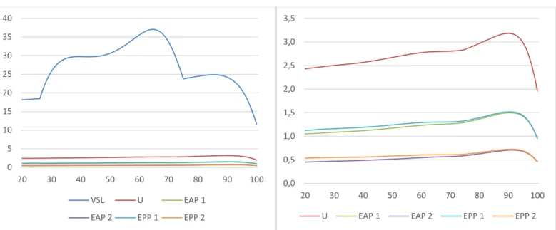
and baseline risk. Section 5 undertakes an empirical exercise, based on the U.S. population survival curve and income distribution, to illustrate the SVRRi concept and to estimate the

impact of age and income on SVRRi and VSLi.

Our headline results are as follows. First, we demonstrate that the SWF framework—by contrast with BCA—provides a rigorous basis for the “fair innings” concept. The social value of risk reduction (SVRR), as calculated using an ex ante or ex post prioritarian SWF, gives extra social weight to risk reduction for younger individuals above and beyond the additional weight they receive in virtue of greater life expectancy remaining. (In an important article, Williams [1997] proposes to operationalize the “fair innings” concept via a non-utilitarian SWF applied to individuals’ quality-adjusted life expectancies; but Williams does not develop this proposal formally, as we do here.)

Second, we show that the manner in which BCA values risk reduction is significantly different from the SWF framework, regardless of which SWF is used (utilitarian, ex ante prioritarian, ex post prioritarian). These differences are multifold. The prioritarian SVRRs display Priority for the Young and Ratio Priority for the Young, while VSL does not. Further, as established in Section 4, the comparative statics of VSL with respect to income and baseline risk are different not only from the ex ante and ex post prioritarian SVRRs, but also from the

utilitarian SVRR. Finally, Section 5 demonstrates that these analytic differences may be empirically quite significant. In particular, VSL increases much more steeply with income in each age group than the utilitarian SVRR, while the prioritarian SVRRs are flat or decrease with income.8

The text of the Article sets forth our analytic apparatus, defines relevant concepts, states our analytic results (as numbered propositions), and interprets these findings or explains the intuition behind them. However, so as to limit the length of the Article and increase readability, we do not include proofs of these propositions in the text. Instead, proofs are provided in an on-line Appendix.

This Article was drafted prior to the coronavirus pandemic of 2020. How to choose fatality-risk-reduction policies was an important topic before the pandemic, and will remain so

7 _{The utilitarian SVRR also does not display Priority for the Young and Ratio Priority for the Young, but this is true}

by definition—since these properties are defined relative to a utilitarian baseline. See Section 3.

8 _{The properties of the ex ante prioritarian and ex post prioritarian SVRRs depend, to some extent, on which concave}

transformation function is used—embodying the degree of priority for the worse off. Thus, in Section 5, the prioritarian SVRRs with a moderately concave transformation function are flat with income, while the prioritarian SVRRs with a more concave transformation decrease with income.

6

after the pandemic abates. But the terrible events of 2020 underscore the significance of the questions we address here. One issue that quickly became salient as Covid-19 cases exploded was risk allocation. Which Covid-19 patients should take priority in receiving scarce medical equipment that would reduce the risk of dying from the disease, such as ventilators? Which uninfected individuals should go to the front of the line in receiving scarce protective equipment, such as N95 masks? The SWF framework provides a systematic methodology for answering such questions. It gives guidance in determining how the social value of reducing an

individual’s fatality risk (in these cases, her risk of dying from Covid-19) should vary, or not, depending upon her age, income, and other characteristics. Understanding these relative social valuations, for three major SWFs—utilitarian, ex ante prioritarian, and ex post prioritarian—is precisely the topic of this Article.

2. Conceptual Framework

2.1 Model of the Population

There is a population of N individuals. The life of a given individual i is divided into periods 1, 2, …, t, …, T, with T the maximum number of periods that any individual can live. Each individual is characterized by an age, risk profile, and income profile, to be explained momentarily.

Calendar time is divided into the present time (also referred as the “current” time), earlier times (“the past”), and later times (“the future”). This enables us to endow each individual i with an “age,” denoted as Ai. We assume that individuals’ periods are synchronized, such that the

present time is the beginning of some period for each of the N individuals. Ai is the number of

the present period for individual i. For example, if Betty has already lived 4 periods, and the present time is the beginning of period 5 of Betty’s life, then ABetty = 5, i.e., Betty’s “age” is 5.9 Ai ≤ T and we also assume that Ai ≥ 2.10

Death and survival are conceptualized as follows. Consider a given individual i and some period t in her life. Assuming the individual is alive at the beginning of period t, she may either die before the period ends, or survive to the end of the period (equivalently, be alive at the beginning of the following period). Let pi(t) denote individual i’s probability of surviving to the

end of period t, conditional on being alive at the beginning of period t. We’ll generally refer to

pi(t) as a “survival probability.” Individual i is characterized by a vector of such probabilities,

one for each period up to T—for short, her “risk profile.”

9 _{Note that our definition of individual i’s “age” as A}

i is slightly different from the colloquial use of the term “age.”

If Betty is at the beginning of the period 5 of her life, then (colloquially) we would say that her age is 4, not 5. However, we need a natural-language term to refer to Ai, and “age” is the most natural choice. The issue here is

purely semantic. Referring to Ai as individual i’s “age” rather than “age plus one” makes no difference to our

analytic results.

10 _{See below, note 22, for an explanation why we assume that A}

7

In our model, these probabilities do not change as the individual ages. Individual i is endowed at birth with survival probabilities for each period t = 1, …, T; and pi(t) at the present

time, the beginning of period Ai, is this at-birth probability.11

Let πi(t; t*) denote individual i’s probability of surviving to the end of period t of her life,

conditional on being alive at the beginning of period t*. In particular, πi(t; Ai) is individual i’s

probability of surviving to the end of period t of her life, conditional on being alive at the

beginning of period Ai—that is, her probability of surviving to the end of period t, conditional on

her current age (Ai). If t < Ai, πi(t; Ai) = 1. If t ≥ Ai, ( ; ) ( )

i t i i i s A t A p s   



Finally, let μi(t; t*) denote individual i’s probability of living exactly t periods,

conditional on being alive at the beginning of period t*. That is, μi(t; t*) is the probability,

conditional on being alive at the beginning of period t*, of surviving through the end of period t and then dying before the end of the next period. In particular, μi(t; Ai) is the individual’s

probability of living exactly t periods, conditional on being alive at the beginning of period Ai—

conditional on her current age.

If t < (Ai – 1), μi(t; Ai) = 0. If t = (Ai −1), μi(t; Ai) is the individual’s probability,

conditional on her current age, of not surviving the current period and instead living exactly (Ai –

1) periods. That is μi(Ai − 1; Ai) = 1 – pi(Ai). Finally, if t ≥ Ai, we have that:

( ; ) ( ; )(1 ( 1)) i t Ai i t Ai p ti

    .

The earnings process is as follows: if an individual survives to the end of period t, she earns an income amount yi(t) > 0. Individual i, thus, is characterized by a vector of incomes,

(yi(1), …, yi(T))—her “income profile.” An individual’s income profile, like her risk profile, is

(in our model) given to the individual at birth and does not change as she ages.12

Period consumption, like period income, is modelled as occurring only if the individual survives to the end of the period. An individual’s consumption during period t, if she survives to the end of period t, is denoted ci(t). We assume “myopic” consumption: ci(t) = yi(t). The

11 _{A different way to model an individual’s fatality risks over the life course would be to conceptualize p}

i(t) as the

currently known conditional probability of i’s surviving period t, given that she is alive at the beginning of that period. On this approach, pi(t) = 1 for t < Ai, since i knows she has survived to the beginning of period Ai.

Modelling fatality risks this way would not change our results, since the formulas for the utilitarian, ex ante prioritarian, and ex post prioritarian SVRRs, and for VSL, do not depend upon past survival probabilities; and because currently known survival probabilities for the present and future periods are the same as at-birth survival probabilities (see Appendix).

We assume 0 < pi(t) < 1 for all t such that 1 < t ≤ T; and that pi(1) = 1. As discussed below, note 22, we

assume that Ai ≥ 2 for all i—that is, that every individual has survived to the end of the first period of her life—and

to ensure this we assume pi(1) = 1. Finally, pi(T + 1) = 0. (This is the probability that i survives one more period,

given that she has survived to the end of period T, the maximum number of possible periods.)

12 _{Of course, if t and t* are distinct periods, then it may well be the case that y}

i(t) ≠ yi(t*). But the profile of incomes

(yi(1), …, yi(T))—specifying, for each period, what the individual will earn at the end of that period if she survives

8

individual consumes in each period whatever she earns then, rather than saving earnings for future consumption or financing consumption by borrowing against future earnings.

“Myopic” consumption might occur because of imperfect markets—the individual lacks access to the financial instruments enabling her to save and borrow—or because of myopic thinking on the individual’s part. Given length constraints, we do not here analyze SVRRi with

a multiperiod model and individual saving and borrowing. This is an important topic for future research.13

Individuals have a common lifetime utility function U(∙), defined as the discounted sum of period utility. Let u(∙) be the common period utility function and β = 1/(1 + φ), φ ≥ 0 the constant utility discount rate. Ui(s) denotes the individual’s lifetime utility if she lives exactly s

periods. 1 ( ) s t ( ( )) i i t U s







Note that the above formula for lifetime utility includes a term for a given period t iff15

the individual survives to the end of the period. If she doesn’t survive to the end of a given period, her period utility is zero. Further, our analysis presupposes that, if i does survive to the end of period t, with consumption ci(t) in that period, u(ci(t)) > 0. Note that if u(ci(t)) < 0,

increasing pi(t) may have the effect of lowering i’s expected lifetime utility. We wish to focus

here on the case in which risk reduction is beneficial to individuals—not the unusual case in which it may be harmful.16

We use Vi to denote the expected lifetime utility of individual i, given his age, risk

profile, and income profile.

1 ( ; ) ( ) i T i i i i t A V  t A U t  





Given that i is alive at the beginning of period Ai, the possible lifespans for him are (Ai −1), Ai,

…, T. The immediately preceding formula aggregates over these possible lifespans, calculating the lifetime utility for each possible lifespan and multiplying each possible lifetime utility Ui (t)

by its probability. A different formula for Vi, useful in calculations, can also be derived (see

Appendix). 1 1 ( ( )) ( ; ) ( ( )) i i A T t t i i i i i t t A V  u y t  t A  u y t   







13 _{In the working paper upon which the current Article is based, we do address the topic of SVRR}

i with saving and

borrowing, although do not undertake a comprehensive analysis. See Adler, Ferranna, Hammitt and Treich (2019).

14 _{Since consumption occurs at the end of each period, the discount factor β is raised to the power t rather than (t−1).} 15 _{“iff” means “if and only if.”}

16 _{In order to ensure that u(c}

i(t)) > 0 for all i and t, we assume that there is a “subsistence” level of consumption czero

such that u(czero_{) = 0 and that y}

9

of i surviving to the end of that period, conditional on his current age;17 _{and sums up over all the}

periods.

2.2 Social Welfare Functions (SWFs)

We’ll use the term “policy” to mean some course of action or inaction by the government. The status quo, therefore, is a “policy”: government chooses not to change individuals’ risk profiles or income profiles. A policy intervention, relative to the status quo, is also a “policy”: government changes individuals’ risk profiles and/or income profiles,

specifically by changing present survival probabilities, future survival probabilities, present income amounts, and/or future income amounts. An individual’s risk profile or income profile with a given policy P is denoted with the superscript “P.” Thus P( )

i

p t is i’s survival probability

in period t with policy P and P( ) i

y t is her period t income with policy P.

The SWF framework has three components: an interpersonally comparable well-being measure, which converts each possible outcome (a possible social consequence) into a vector of well-being numbers, one for each of the persons in the population; a rule for ranking well-being vectors; and an uncertainty module, namely a procedure for applying the rule to policies

understood as probability distributions across outcomes. (Adler 2012, 2019.) If individuals have a common utility function, then the well-being measure can be equated with that utility function (which is the approach we follow here). (Adler 2019, ch. 3, app. D.) In what follows, we use “SWF” to mean the combination of a rule for ranking well-being vectors and an uncertainty module for that rule.

We consider three SWFs: the utilitarian SWF, the ex ante prioritarian SWF, and the ex post prioritarian SWF. Each assigns a score (a real number) to a given policy P, and ranks policies in the order of these scores. We’ll denote the utilitarian SWF as WU_{(∙), the ex ante}

prioritarian SWF as WEAP_{(∙), and the ex post prioritarian SWF as W}EPP_{(∙)—or, more compactly,}

as WU_{, W}EAP_{, and W}EPP_{. We’ll use W(∙) as a generic term to indicate any SWF, with W(∙) then}

specified as WU_{, W}EAP_{, W}EPP_{, or as some other SWF.}18

The utilitarian rule ranks well-being vectors according to the sum of well-being. The standard procedure for applying the utilitarian rule under uncertainty is to sum individuals’ expected well-being. This yields the utilitarian SWF.

Definition 1a: The Utilitarian SWF. U( ) N₁ P i i W P 



i for a given W(∙) is the partial derivative of W(∙) with respect to i’s current survival probability. See Section

2.3. In order for this partial derivative to be well-defined, the SWF needs to be score-based, as are WU_{, W}EAP_{, and}

WEPP _{(assigning a real number to each policy and ranking policies in the order of those numbers), and indeed}

10

The prioritarian rule ranks well-being vectors according to the sum of a strictly increasing and strictly concave transformation of individual well-being. Let g(∙) denote some strictly

increasing and strictly concave function. By summing g(∙)-transformed well-being numbers, the prioritarian rule has the effect of giving greater weight to well-being changes affecting worse-off individuals. Assume that in well-being vector w a better-off individual is at well-being level wH,

and a worse-off individual is at well-being level wL, with wH > wL. Let ∆w > 0 be a change in

being. Well-being vector w* is identical to w, except that the better-off person is at well-being level wH + ∆w. Well-being vector w** is identical to w, except that the worse-off person

is at well-being level wL + ∆w. The utilitarian rule is indifferent between w* and w**, while the

prioritarian rule prefers w**, by virtue of the strict concavity of g(∙). It prefers to give a fixed increment in well-being to a worse-off person rather than to a better-off one.

The two main approaches to applying the prioritarian rule under uncertainty are ex ante prioritarianism and ex post prioritarianism.19 _{(Adler 2012, ch. 7; Adler 2019, app. J; Adler}

Hammitt and Treich 2014.) Ex ante prioritarianism assigns a score to a given policy by

calculating expected well-being for each individual; applying the transformation function, g(∙), to each individual’s expected well-being; and then summing up these g(∙)- transformed well-being expectations. Ex post prioritarianism assigns a score to a given policy by taking the expected value, for each individual, of her g(∙)-transformed well-being; and summing up these expected transformed well-being numbers.20 _{In a nutshell, the ex ante prioritarian formula is the sum}

across individuals of transformed expected well-being, while the ex post prioritarian formula is the sum across individuals of expected transformed well-being.

Ex ante and ex post prioritarianism each have a central place in the literature on

prioritarianism because each has axiomatic advantages compared to the other. It can be shown that no procedure for applying the prioritarian rule under uncertainty can satisfy both the ex ante Pareto axioms, and a very plausible axiom of stochastic dominance. Ex ante prioritarianism satisfies the ex ante Pareto axioms, but violates stochastic dominance; ex post prioritarianism satisfies stochastic dominance, but violates the ex ante Pareto axioms.21 _{(Utilitarianism satisfies}

19 _{The choice between ex ante and ex post approaches to equity has also been discussed in health economics.}

(Bleichrodt 1997).

20 _{The rule for ex post prioritarianism is often stated in a different way: as the expected value of the sum of}

individuals’ transformed well-being. But this is mathematically equivalent to the rule stated in the text: the expected value of the sum of individuals’ transformed being equals the sum of individuals’ expected transformed well-being. (Adler 2019, app. J).

21 _{The ex ante Pareto axioms are Ex Ante Pareto Indifference and Ex Ante Strong Pareto. Ex Ante Pareto}

Indifference: If each person’s expected well-being with policy P is equal to her expected well-being with policy P*, then P and P* are equally good. Ex Ante Strong Pareto: If each person’s expected well-being with policy P is greater than or equal to her expected well-being with policy P*, and at least one person’s expected well-being is strictly greater, then P is better than P*. Stochastic Dominance: If, for each possible state of nature, the well-being vector produced by policy P in that state is better than the well-being vector produced by policy P*, then P is better than P*. On the axiomatic properties of utilitarianism and prioritarianism under uncertainty, see generally Adler 2012 ch. 7; Adler 2019 ch. 3-4, apps. I-L.

11

the ex ante Pareto axioms and stochastic dominance, but lacks the extra weighting for the worse off that is characteristic of prioritarianism, and that its proponents find to be ethically attractive.)

In the model here, the formulas for ex ante and ex post prioritarianism are as follows. Definition 1b: The Ex Ante Prioritarian SWF.

1 ( ) N ( ) EAP P i i W P 



Definition 1c: The Ex Post Prioritarian SWF.

1 1 ( ) ( ; ) ( ( )) i N T EPP P P i i i i t A W P  t A g U t    

 

with g(∙) a strictly increasing and strictly concave function.

The utilitarian SWF is a specific SWF (a specific formula for ranking policies as a function of individuals’ ages, risk profiles, and income profiles) while the ex ante prioritarian SWF and ex post prioritarian SWF are, each, families of SWFs. The choice of a particular strictly increasing and strictly concave g(∙) defines a specific WEAP _{and W}EPP_{. Our analysis will}

be generic, holding true for any g(ꞏ). We do assume that g(ꞏ) is twice differentiable, so that g′(ꞏ) > 0 and g′′(ꞏ) < 0.22

Note that all three SWFs are defined in terms of individuals’ lifetime well-being. WU

calculates each individual’s expected lifetime well-being, and sums across individuals. WEAP

calculate each individual’s transformed expected lifetime well-being, and sums across individuals. WEPP _{calculates each individual’s expected transformed lifetime well-being, and}

sums across individuals. The application of SWFs to lifetime well-being has a strong ethical justification. (Adler 2012, ch. 6). While much of the SWF literature uses one-period models for reasons of tractability, there is also a significant body of work using multiperiod or lifetime numbers as the input to an SWF.23 _{(For discussion of this literature, see Adler [2012, p. 245];}

Boadway [2012, pp. 86-106]; Tuomala [2016, pp. 360-64].)

2.3 The Social Value of Risk Reduction (SVRR)

22 _{The “Atkinson” family of g(∙) functions—g(u) = (1−γ)}−1_u1−γ_{, γ > 0, γ ≠ 1; and g(u) = ln u if γ = 1—have attractive}

axiomatic properties and are regularly used in the economic literature on prioritarianism. See Adler (2012, ch. 5). (Indeed our empirical exercise in Section 5 uses an Atkinson g(∙) function.) The Atkinson g(∙) is such that g(0) is undefined for γ ≥ 1. In order for our analysis to accommodate the possibility that g(0) is undefined, we assume that

Ai ≥ 2 for all i. (Note that the expression for the ex post prioritarian SWF in Definition 1c includes the g(∙) value of

individual i’s lifetime well-being if she lives exactly (Ai −1) periods. If Ai = 1, the individual’s lifetime well-being if

she lives exactly Ai – 1 periods is 0.) Because the period length can be arbitrarily short, the assumption that Ai ≥ 2

is not significantly restrictive.

23 _{Similarly, while much empirical work on income inequality focuses on annual income, there is also a significant}

body of work that looks at the inequality of lifetime income. See, for example, Bönke et al. (2015), Bowlus and Robin (2004), Guvenen et al. (2017), Huggett et al. (2011), Nilsen et al. (2012).

12

We’ll use the “O” superscript to denote an individual’s status quo income and risk profiles: piO(t) is individual i’s status quo survival probability for period t and yiO(t) her status

quo income for period t.

Assume that government enacts a policy intervention, relative to the status quo, at the beginning of the current period. Among other effects, the policy may change individual i’s current survival probability. Let Δpi be this change: i’s current survival probability in the status

quo is piO(Ai) and her current survival probability after the intervention is piO(Ai) + Δpi.

We can now define SVRRi, which will be useful in understanding the impact of this

policy intervention on social welfare.

Definition 2: The Social Value of Risk Reduction (SVRRi). SVRRi for a given SWF W(∙) is the partial derivative

( ) i i

W p A



 evaluated at i’s status quo risk and income profile.24 By the total differential approximation from calculus, the change in social welfare resulting from Δpi is approximately SVRRi Δpi.25

Intuitively, SVRRi is the change in social welfare per unit of current risk reduction for

individual i, as calculated for a marginal such reduction. To be sure, a governmental policy intervention may well have effects other than changing individuals’ current survival

probabilities. It may also change their survival probabilities in future periods. And a risk-reduction intervention will surely have costs, which will be reflected in a change to individuals’ current and/or future incomes. The total effect of a policy intervention on social welfare will be approximately equal to the sum, across individuals, of SVRRi Δpi plus corresponding terms for

changes to future survival probabilities and to incomes. SVRRi captures that portion of a policy

intervention’s total impact on social welfare that results from the change to individual i’s current survival probability. 24 _{Formally, ( (1),..., ( ); (1),..., ( ))} ( ) O O O O i i i i i i i W SVRR p p T y y T p A  

 . Since all three SWFs are additively separable across individuals, ( ) i i W p A 

 can be expressed just as a function of i’s risk and income profiles; the value of this partial derivative does not depend upon other individuals’ risks and incomes.

25 _{Assume that a policy intervention changes individual i’s current survival probability by ∆p}

i; her survival

probability in period t by ∆pit, with t > Ai; and her income in period t by ∆yit, with t ≥ Ai. Then, by the

total-differential approximation from calculus, ∆W is approximately equal to:

1 ( (1),..., ( ); (1),..., ( )) ( (1),..., ( ); (1),..., ( )) ( ) ( ) i i T T O O O O t O O O O t i i i i i i i i i i i i i t A _i t A _i W W SVRR p p p T y y T p p p T y y T y p t y t                _     







13

Further, by comparing SVRRi to SVRRj, for two individuals i and j—as we do below—

we can determine the relative social impact of risk reductions for the two. Consider a change ∆p to someone’s current survival probability. That risk change, if accruing to individual i, results in a change of social welfare by approximately SVRRi Δp. If accruing to individual j, it results in

a change of social welfare by approximately SVRRj Δp. Thus (for a small ∆p) the first social

welfare change is larger than/smaller than/equal to the second iff SVRRi is larger than/smaller

than/equal to SVRRj.

SVRRi is defined (Definition 2) as the partial derivative of the SWF with respect to

individual i’s current survival probability, with this partial derivative evaluated at individual i’s status quo risk and income profiles. This reference to the status quo doesn’t limit the generality of the definition. For any assignment of income and risk profiles to individuals, we can take that assignment as the status quo and consider the social welfare impact of policy interventions relative to that baseline.

As a notational matter, we’ll also denote SVRRi for a generic SWF W(∙) as Si; and SVRRi

for WU_{, W}EAP_{, and W}EPP _{specifically as (respectively)} U i S , EAP i S , and EPP i S .

Using the definition of SVRRi and of the SWFs (Definitions 1a, 1b, 1c), it is

straightforward to calculate U i S , EAP i S , and EPP i S .26 Proposition 1a. ( 1) ( ; ) ( ) ( ) i O T U O i i O i i i O i t A i i t A S U A U t p A









We can provide intuitive explanations for these formulas, beginning with the utilitarian SVRRi. Observe that S is equal to the difference between (1) individual i’s expected lifetime U_i

well-being conditional on surviving the current period, i.e., ( ; ) ( ) ( ) i O T O i i i O t A i i t A U t p A  



realized lifetime well-being if she dies during the current period (does not survive it), i.e., ( 1)

O i i

U A .

Consider the simple case in which individual i would die for certain during the current period, absent governmental intervention, and intervention ensures that she survives the period. In this case, clearly, the change in utilitarian social welfare that results from the intervention is

14

the difference between individual i’s expected lifetime well-being conditional on surviving the current period, and her realized lifetime well-being if she dies during the current period. For short, let’s term this difference the “utilitarian gain from saving individual i.”

More generally, consider a policy which increases individual i’s current survival probability by ∆pi. The change in utilitarian social welfare that results from the ∆pi increase is

just ∆pi multiplied by the utilitarian gain from saving individual i. ThusS , the marginal change _iU

in utilitarian social welfare per unit of current-period risk reduction for individual i, is nothing

other than ( 1) ( ; ) ( ) ( ) i O T O i i O i i O i t A i i t A U A U t p A



  



The formula for the ex ante prioritarian SVRRi, S_iEAP, is the utilitarian SVRRi multiplied

by a weighting factor, ( O) i

g V . This weighting factor is a function of the individual’s expected lifetime well-being, and decreases as expected lifetime well-being increases. It reflects the priority given by the ex ante prioritarian SWF to individuals at lower levels of expected lifetime well-being.

Finally, the formula for the ex post prioritarian SVRRi, S_iEPP, is the same as that for the

utilitarian SVRRi, except that transformed lifetime well-being, g(Ui), is substituted for lifetime

well-being Ui. Consider the case in which individual i would die for certain during the current

period, absent governmental intervention, and intervention ensures that she survives the period. In this case, the change in ex post prioritarian social welfare that results from the intervention is the difference between individual i’s expected transformed lifetime well-being conditional on surviving the current period, ( ; ) ( ( ))

( ) i O T O i i i O t A i i t A g U t p A





i i

g U A

  . For short, let’s term this difference the “ex post prioritarian gain from saving individual i.”

More generally, consider a policy which increases individual i’s current survival probability by ∆pi. The change in ex post prioritarian social welfare that results from the ∆pi

increase is just ∆pi multiplied by the ex post prioritarian gain from saving individual i. Thus

EPP i

S , the marginal change in ex post prioritarian social welfare per unit of current-period risk reduction for individual i, is nothing other than the ex post prioritarian gain from saving individual i.

Note that our assumption that u(yi(t)) > 0 for all i, t—it is always better to survive a

period than to die before its end—ensures that U i

S , EAP

i

S , and EPP i

S > 0 for all i. Risk reduction is always a social benefit—whether social benefits are calculated using a utilitarian, ex ante prioritarian, or ex post prioritarian SWF.

15

It would be of interest to consider the relation between SVRRi as defined here and the

partial derivative of the SWF with respect to future survival probability. Given space

constraints, we do not address this topic, and instead focus in this Article on how the marginal social welfare impact of changes to current survival probability varies among individuals as a function of their ages, income profiles, and risk profiles.

2.4 Benefit-Cost Analysis (BCA) and the Value of Statistical Life (VSL)

BCA is an evaluation methodology that assigns a score to each policy by summing up individuals’ monetary equivalents for that policy. (Adler 2012, pp. 88-114; Boadway 2016). In the model here, MEi(P), individual i’s monetary equivalent for policy P, is the change to her

current status quo income that equalizes her expected utility as between the policy and the status quo. We use B(∙) to denote the BCA methodology. B(P) is the score assigned by BCA to policy

P: the sum of monetary equivalents for P.

Definition 3: Benefit-Cost Analysis. B P( )



defined in the accompanying footnote.27

The value of statistical life (VSL) is standardly defined as the marginal rate of

substitution between an individual’s material resources (wealth, income, or consumption) and survival probability. (Eeckhoudt and Hammitt 2001; Evans and Smith 2006; Kaplow 2005; Hammitt 2007.)

Consistent with this general approach, we define VSLi in our model as follows.

Definition 4: The Value of Statistical Life (VSLi). / ( )

/ ( ) i i i i i i i V p A VSL V y A      , with these partial derivatives evaluated at i’s status quo risk profile and income profile.28

27 _{Let ( (1),..., ( ); (1),..., ( ))}

i i i i i

V p p T y y T denote individual i’s expected lifetime utility as a function of risk profile

(pi(1), …, pi(T)) and income profile (yi(1), …, yi(T)). That is,

1 1 ( ; ) ( (1),..., ( ); (1),..., ( )) ( ( )) ( ( )) i i T i i t A A t i i i i i i t t i t A V p p T y y T u y t   u y t    







= ∆y such that:

( O(1),..., O( ); O(1),..., O( 1), O( ) , O( 1),..., O( )) ( P(1),..., P( ); P(1),..., P( ),..., p( ))

i i i i i i i i i i i i i i i i i i

V p p T y y A y A  y y A  y T V p p T y y A y T

.

Note that MEi(P), thus defined, is individual i’s “equivalent variation” for policy P. Sometimes, BCA is

defined instead as the sum of “compensating variations.” (Boadway 2016; Freeman 2003, ch. 3.) There are theoretical advantages to conceptualizing monetary equivalents for purposes of BCA as equivalent variations rather than compensating variations. (Adler, Hammitt and Treich 2014, n. 8.) However, that choice is not significant for purpose of this Article. Whether monetary equivalents are defined as equivalent variations or compensating variations, ( ) i i i B VSL p A    . See Appendix.

16

The relation between VSLi and B is directly analogous to the relation between SVRRi and W. Just as ( ) i i i W SVRR p A    , so i _i( )_i B VSL p A  

 . This was true in the one-period model analyzed in Adler, Hammitt and Treich (2014), and remains true in the lifetime model under consideration here. Proposition 2a. ( ) i i i B VSL p A    , with _i( )_i B p A 

 evaluated at i’s status quo income and risk profiles.

Intuitively, VSLi is the marginal change in the sum of monetary equivalents per unit of

current risk reduction for individual i, just as SVRRi is the marginal change in social welfare per

unit of current risk reduction for individual i. Assume that a policy intervention changes individual i’s current survival probability by ∆pi. While the change in social welfare resulting

from this risk change is approximately SVRRi Δpi, the change in the sum of monetary

equivalents is approximately VSLi ∆pi.29

From Definition 4, plus the formulas above for Vi and the utilitarian SVRRi, it is

straightforward to derive that VSLi equals the utilitarian SVRRi (S ) divided by the expected _iU

marginal utility of i’s current income.

Proposition 2b. ( ) i ( ( )) U i i O A O i i i i S VSL p A  u y A  

28 _{To state this definition more formally, let V}

i be expressed as a function of individual i’s risk profile and income

profile, as in note 24 immediately above. V_i V p_i( _i(1),...,p T y_i( ); _i (1),...,y T_i ( )). Then VSLi =

( (1),..., ( ); (1),..., ( )) ( (1),..., ( ); (1),..., ( )) ( ) ( ) O O O O O O O O i i i i i i i i i i i i i i V V p p T y y T p p T y y T p A y A     .

Adler, Hammitt and Treich (2014), using a one-period model, defined VSL as the marginal rate of substitution between survival probability and wealth. In the multi-period model with myopic consumption that we use in this Article, an individual’s wealth in each period is zero—she consumes what she earns and saves nothing— and so VSL is here defined as the marginal rate of substitution between survival probability and income or, equivalently, consumption.

29 _{As in note 23 above, consider a policy intervention that changes individual i’s current survival probability by ∆p}

i;

her survival probability in period t by ∆pit, with t > Ai; and her income in period t by ∆yit, with t ≥ Ai. Again using

the total-differential approximation from calculus, ∆B is approximately equal to:

1 ( (1),..., ( ); (1),..., ( )) ( (1),..., ( ); (1),..., ( )) ( ) ( ) i i T T O O O O t O O O O t i i i i i i i i i i i i i t A _i t A _i B B p p p T y y T p p p T y y T y p t y t VSL                     







. The terms in this equation for the partial derivative of B(∙) with respect to survival probability in a future period

t—that is ( ) i B p t 

 , t > Ai—can also be related to VSLi. It can be shown that each such term equals VSLi multiplied by the marginal rate of substitution with respect to Vi between present survival probability and survival probability

17

Given the formula for VSLi stated in Proposition 2b, it can be observed that the

comparative statics of VSLi and the utilitarian SVRRi will be the same in the special case where

all individuals in the status quo have the same expected marginal utility of current income. In that case, the denominator in this formula will be the same for all individuals, and VSLi then

equals U i

S multiplied by a common positive constant. In general, however, relative to a generic

status quo, VSLi and S do not have the same comparative statics—as our analysis in Sections 3 _iU

and 4 below will demonstrate.

If we posit a perfect tax system that redistributes income so as to equalize individuals’ expected marginal utilities of (after-tax) present income, then the comparative statics of VSLi

and U i

S will be the same. Observe, here, that equalizing incomes does not necessarily equalize

expected marginal utilities of after-tax present income—since, for example, two individuals of the same age with the same after-tax present income but differing survival probabilities for the current period will have different expected marginal utilities.

A terminological note. We use the terms “SVRRi” and “VSLi” as the names for the

concepts defined in Definitions 2 and 4 so as to emphasize that SVRRi and VSLi values are

individual-specific. In general, given two distinct individuals i and j, it need not be the case that SVRRi = SVRRj and it need not be the case VSLi =VSLj. However, in what follows, so as to

reduce clutter, we regularly drop the “i” subscript and use “SVRR” and “VSL” as shorthand, respectively, for “SVRRi” and “VSLi.”

3. Age Effects and “Priority for the Young”

The effect of age on the SVRR has never been addressed by the academic literature. In this Section, we analyze what our model implies with respect to age effects on SVRR as well as VSL by considering two individuals i and j, with identical risk profiles and income profiles, but the first older than the second (Ai > Aj).

Both SVRRi and VSLi are determined by individual i’s status quo income profile and risk

profile. (See Propositions 1a, 1b, 1c, 2b.) Thus, in analyzing the properties of SVRRi and VSLi

in this Section as well as Section 4, we will not need to refer to incomes or probabilities, or to utilities as a function of incomes and probabilities, other than status quo values. We therefore remove the “O” superscript on incomes, probabilities, and utilities, which is implicit. yi(t)

denotes O( )

i

y t , pi(t) denotes p t , V_iO( ) i denotes V , and so forth. Further, we often drop _iO

subscripts on incomes or probabilities where these are the same for i and j, e.g., y(t) indicates

yi(t) =yj(t).

18 What are the relative magnitudes of U

i

S andSUj , for two individuals of different ages (Ai

> Aj) but with identical risk and income profiles? In other words, how does the utilitarian gain

from saving an individual depend upon her age? It can be shown that SU_j S_iUequals:









Thus the utilitarian SVRR decreases/is unchanged/increases with age iff the value of this formula is positive/zero/negative.

The first term in this formula (for short, the “duration term”) is positive. By increasing the younger individual’s current survival probability, we increase her chance of surviving the periods Aj, Aj +1, …, Ai – 1 in her life, and that probability change for each such period yields an

increment in expected lifetime well-being (by increasing her chance of accruing consumption utility with respect to that period). This increment to expected lifetime well-being with respect to periods Aj, Aj +1, …, Ai – 1 does not occur if we increase the older individual’s survival

probability, since he has already survived those periods.

The second term in the formula above (for short, the “risk term”) is negative. By

increasing either individual’s current survival probability, we increase that individual’s chance of surviving periods Ai, Ai + 1, …, T in his or her life, and thereby increase his or her chance of

accruing consumption utility with respect to those periods. The risk term captures the difference between the magnitude of this benefit for the younger individual and its magnitude for the older one. Since the older individual is sure to be alive at the beginning of period Ai, while the

younger individual is not, this difference is negative.

Clearly, if income can increase with age, the magnitude of the risk term may exceed that of the duration term, and thus the utilitarian gain from saving the older individual i may be greater than that of saving the younger one. What if constant income is assumed? With a constant income profile and a constant risk profile, the duration term predominates and the utilitarian SVRR decreases with age. More generally, it can be shown that if the income and risk profiles are such that income does not increase with age and survival probabilities do not

increase with age, then the utilitarian SVRR decreases with age. (See Appendix.) 3.2 Age Effects and the Ex Ante Prioritarian SVRR

A simple manipulation shows that EAP EAP ( )









j i j j i i j i

S S  g V S S S g V g V .

We noted immediately above in discussing the utilitarian SVRR that the quantity( U U)

j i

S S

19 namely ( )





j j i

g V S S , incorporates those terms. This part is positive iff ( U U)

j i

S S is

positive. The second part of the formula here, U





i j i

S g V g V , is a third term (“priority for the young”), which is always positive. Because Vi > Vj (the older individual has greater expected

lifetime well-being) and g(ꞏ) is strictly concave, g′(Vi) < g′(Vj).

The intuition behind the formula is as follows. Ex ante prioritarian social welfare, WEAP_,

is the sum of individuals’ transformed expected lifetime well-beings— transformed by a strictly increasing and strictly concave g(ꞏ) function. The effect of this transformation is to give greater social weight to changes in expected lifetime well-being that accrue to individuals at a lower level of expected lifetime well-being. The differential ex-ante-prioritarian benefit of saving a younger rather than older individual reflects the differential gains to expected lifetime well-being of saving the younger one ( U U)

j i

S S . But it also reflects the fact that the younger individual has a lower level of expected lifetime well-being and thus takes priority ( ( )g V _j g V( )_i ).

We now define “Priority for the Young” more formally.

Definition 5: Priority for the Young. Consider any two individuals i and j with identical risk profiles and income profiles (pi(t) = pj(t) and yi(t) = yj(t) for all t), and such that Ai > Aj. SVRRfor a given SWF W(∙) displays “Priority for the Young” iff the following is

true for any such i and j: U U 0 0

j i j i

S S   S S  . Similarly, VSL displays Priority for the Young iff the following is true for any such i and j: U U 0 0

j i j i

S S  VSL VSL  .

Priority for the Young is a precise expression, using the SVRR formalism, of the fair innings concept. Recall our informal definition of “fair innings” in the Introduction (Section 1): As between a policy that produces a given gain in expected lifetime well-being for a younger person, and an otherwise-identical policy that produces the same gain in expected lifetime well-being for an older person, it is ethically better for society to undertake the first policy. Recall too (Section 3.1) that the utilitarian SVRRi, S , is equal to the per-unit gain to expected lifetime _iU

well-being from reducing i’s current fatality risk. If i’s current survival probability increases by ∆pi, his expected lifetime well-being increases by  p_i S_iU.

If SVRRi for a given SWF W(∙) displays Priority for the Young, then it never assigns a

smaller or equal value to risk reduction for the younger individual if the utilitarian risk-reduction value is larger for the younger than for the older individual. (If the SWF displays Priority for the Young, it follows that: U U 0 0

j i j i

S S  S S  .) Further, if the utilitarian risk-reduction values are equal, the SWF places a larger value on risk reduction for the younger individual. (If the SWF displays Priority for the Young, it also follows that: U U 0 0

j i j i

20

Proposition 3a. The Ex Ante Prioritarian SVRR displays Priority for the Young. We can illustrate why ex ante prioritarianism satisfies Priority for the Young using the Bognar (2015) thought experiment presented in the Introduction. Consider two patients, a young patient j and an older patient i, who are respectively at the beginning of periods two and three of their lives. The maximum lifespan is three periods. The patients have a common risk profile, with p2 the common survival probability for period two and p3 the common survival probability

for period three. Assume also that the patients are equally well off, materially. Each faces the same, constant, income profile, with period utility normalized to 1 and a zero utility discount rate.

Finally, assume that p3 is close to zero, so that SU_j S_iU 1(as shown in note 27). Thus,

if we have one dose of a drug that can increase a patient’s current survival probability by some fixed increment, utilitarianism is indifferent between giving the drug to the younger or the older patient; the utilitarian SVRRs are approximately equal. However, we easily obtain that

2

(1 ) (2)

EAP EAP

j i

S   g p S  g , by the concavity of g(ꞏ).30 _{Ex ante prioritarianism tells us to}

give the drug to the younger individual, who has a lower expected lifetime well-being (it is uncertain whether she will survive the second period, while the older patient will definitely live at least two periods). Ex ante prioritarianism gives greater weight to a given increase in expected lifetime well-being if it accrues to an individual at a lower level of expected lifetime well-being, and so the younger patient takes priority.

Not only does ex ante prioritarianism satisfy Priority for the Young. We can prove a logically stronger result, namely that the relative social value of risk reduction for young versus old individuals is always greater with ex ante prioritarianism than with utilitarianism.

( EAP/ EAP) ( U/ U)

j i j i

S S  S S . If utilitarianism prefers to reduce the younger individual’s risk (the utilitarian gain from saving her is greater), ex ante prioritarianism has a yet greater degree of priority for the young. If utilitarianism is indifferent (the utilitarian gains are equal), ex ante prioritarianism gives priority to the young. Finally, although ex ante prioritarianism may prefer to reduce the risk of the older individual (if the utilitarian gain from saving her is sufficiently greater), in this case it always gives less priority to the older individual than utilitarianism does.

Definition 6: Ratio Priority for the Young. Consider any two individuals i and j with identical risk profiles and income profiles (pi(t) = pj(t) and yi(t) = yj(t) for all t), and such

that Ai > Aj. SVRRfor a given SWF W(∙) displays “Ratio Priority for the Young” iff the

30 _V

j, the expected lifetime well-being of the younger individual, is (1 – p2) (1) + p2(1 – p3) (2) + p2p3(3) = 1 + p2 +

p2p3; while Vi, the expected lifetime well-being of the older individual, is (1 – p3) (2) + p3(3) = 2 + p3. Thus,

3 2 1 j U j V S p p      , while ₃ 1 U i i V S p     . (1 2 2 3)(1 3) EAP j S g p p p p and EAP (2 ₃) i S g  p .