Collision avoidance via laser rangefinding

(1)

Collision Avoidance via Laser Rangefinding

By

Long N. Phan

Submitted to the Department of Mechanical Engineering In Partial Fulfillment of the Requirements for the Degree of

Bachelor of Science in Mechanical Engineering

and

Master of Science in Mechanical Engineering

at the

Massachusetts Institute of Technology

May 1999 _{autohrby 9r0sd1to M}

Ct*)ronic copies of thS the-si documentn wholo or In pcAs

Author

Obepartment of Mechanical Engineering

Certified by

Paul A. DeBitetto Senior Member of Technical Staff, Charles Stark Draper Laboratory

Certified by

Thesis Supervisor

Sanjay E. Sarma Professor of Mechanical Engineering, Massachusetts Institute of Technology

Th iwarvisor

Accepted by

Ain A. Sonin Chairman, Department Committee on Graduate Theses

SSACHUSETTS IN TI

(2)

Collision Avoidance via Laser Rangefinding

By

Long N. Phan

Submitted to the Department of Mechanical Engineering On May 1, 1999 in Partial Fulfillment of the

Requirements for the Degree of Bachelor of Science

And Master of Science In Mechanical Engineering

Abstract

This thesis describes the design of a prototyped collision avoidance sensor for small autonomous vehicles. The system is based on laser rangefinding using time-of-flight, and built using small, low-cost, off-the-shelf components. The key requirement is for terrain mapping in an urban environment on small autonomous vehicles although it can potentially be used for any application that requires rangefinding. The completed scanning laser rangefinding system includes a high power pulsed laser, high-speed time-of-flight measurement device, optical receiver, some optics, high-speed servo, and a

microcontroller. System performance was characterized for both rangefinding and

scanning functions. The final system design provides operational flexibility and technical knowledge for designing similar rangefinding systems.

Thesis Supervisor: Paul A. DeBitetto

Title: Senior Member of Technical Staff, Charles Stark Draper Laboratory

Thesis Supervisor: Sanjay Sarma

(3)

Acknowledgements

This thesis was prepared at The Charles Stark Draper Laboratory, Inc., under Internal Research & Development No. 18598.

Publication of this thesis does not constitute approval by Draper or the sponsoring agency of the findings or conclusions contained herein. It is published for the exchange and stimulation of ideas.

Permission is hereby granted by the Author to the Massachusetts Institute of Technology to reproduce any or all of this thesis.

Long N. Phan

The work that is described in this document was by no means done all by myself. There are many people that I would like to thank for their support of my education here at MIT and Draper Laboratory during the many years.

First, I would like to thank all the members of the Draper helicopter team. I have been involved with the team for almost five years now and my development as an engineer was largely attributed by members of the team; Paul DeBitetto, Bill Hall, Bob Butler, former Draper Fellow Christian Trott, Michael Bosse, and Rusty Sammon. Big thanks goes to Paul DeBitetto for his support of my wild endeavors, no matter how difficult or challenging the task may be and for guiding my personal growth. Bob Butler provided a lot of electrical engineering help to a young mechanical engineer. Christian Trott and Michael Bosse were student members of the winning 1996 International Aerial Robotics competition and we spent the whole summer sweating and working together under the most extreme of conditions. Rusty Sammon is my partner in the collision avoidance sensor business and supported me technically in every way. Without him, the

sensor would not have been completed.

Other Draper fellows and students in the autonomous vehicle lab include Bill Kaliardos, Charles Tung, Mohan Gurunathan, Anthony Lorusso, and the many others who have come and gone. Bill Kaliardos is a fellow mechanical engineer and mentor with many many years of experience to draw from. His nightly moral support and jokes will be missed. I would like to take this time to thank all the guys in the original unmanned vehicle lab for "lending" me the "tools" over the years and not charging me a premium for it.

From MIT, I would like to thank my good friend, Amy Yu, for helping me get through my years of hardship to get to where I am today. Professor Sarma has been one hell of a professor for helping me in every way a professor could. His excellence and enthusiasm has been absolutely inspiring.

Finally, I would like to thank my entire family for years of encouragement and support. It is to my mother, father, brother, and sister that I dedicate all my effort.

Long N. Phan May, 1999

(4)

Biographical Note

Long N. Phan was born on June 13, 1976 in Saigon Vietnam. He spent two years in his home country before his parents and uncle left the country as boat refugees traveling from country to country to escape the communist state of Vietnam. In December of

1979, his entire family made it safely to the United States where they resided in the

tropical islands of Hawaii. After years of hardship, Long graduated from McKinley High School in Honolulu in 1994 and attended the Massachusetts Institute of Technology studying mechanical engineering as an undergraduate and graduate student. During his years, he was active as a varsity volleyball player, member of the Beta Chapter of the Chi Phi Fraternity, and a competitive engineering student who competed in over three

international engineering competitions. During all his summers, he worked on the

autonomous aerial vehicle project at Draper Laboratory where he focused on electromechanical systems engineering. This work was the focus of his research for almost two years, from the beginning of his senior year to the end of his graduate year. Contingent upon this acceptance of this thesis, Long will be awarded a Bachelor of Science and Master of Science degree in mechanical engineering and minor in economics. His future career plan is to work on Wall Street as a trader for Lehman Brothers.

(5)

List of Figures

FIGURE 2.1 DISPERSION PATTERN FOR POLAROID SONAR... 16

FIGURE 2.2 A TYPICAL SONAR SETUP... 18

FIGURE 2.3 TIMING DIAGRAM FOR ULTRASONIC SONAR ... 18

FIGURE 2.4 POLAROID 6500 SERIES MODULE AND TRANSDUCER ... 19

FIGURE 2.5 MULTISPECTRAL UWB RADAR SYSTEM BLOCK DIAGRAM... 23

FIGURE 2.6 MULTISPECTRAL UWB RADAR SYSTEM ... 23

FIGURE 2.7 MEASURED TIME AND FREQUENCY RESPONSE OF MULTISPECTRAL UWB RADAR ... 24

FIGURE 2.8 M IR M OTION SENSOR ... 27

FIGURE 2.9 M IR M ODULAR RANGEFINDER ... 28

FIGURE 2.10 D IFFUSE REFLECTIONS ... 31

FIGURE 2.11 M IRROR-LIKE REFLECTIONS... 31

FIGURE 2.12 R ETROREFLECTIONS ... 31

FIGURE 2.13 TRIANGULATION TECHNIQUE ... 34

FIGURE 2.14 OBSTRUCTION IN TRIANGULATION... 35

FIGURE 2.15 PULSED LASER SYSTEM ... 36

FIGURE 2.16 CONTINUOUS WAVE PHASE SHIFT LASER RANGEFINDING ... 38

FIGURE 2.17 LEICA OEM COMPARISON TABLE ... 40

FIGURE 2.18 LEICA MRF2000 MONOCULAR RANGEFINDER (LEFT) AND STANDALONE UNIT (RIGHT) ... 40

FIGURE 2.19 RIEGL LASER DISTANCE SENSOR LD90-3GF HEAD UNIT W/O ELECTRONICS... 41

FIGURE 2.20 ACCUITY RESEARCH ACCUIRANGE 4000... 42

FIGURE 2.21 RIEGL MINIATURIZED 2D LASER SCANNER HEAD (LEFT) AND SYSTEM LAYOUT (RIGHT) ... 43

FIGURE 2.22 ACCUITY ACCURANGE 4000 2D LINE SCANNER ... 44

FIGURE 2.23 RIEGL LASER MIRROR SCANNER LMS-Q140-60/80... 46

FIGURE 3.1 SCANNING LASER RANGEFINDING SYSTEM LAYOUT... 49

FIGURE 3.2 SOLAR RADIATION NOISE SPECTRUM ... 50

FIGURE 3.3 POWER TECHNOLOGY PACKAGED PULSE LASER SYSTEMS ... 52

FIGURE 3.4 DIMENSION DRAWINGS OF POWER TECHNOLOGY'S PULSED LASERS... 52

FIGURE 3.5 O PTICAL R ECEIVER ... 55

FIGURE 3.6 BASIC SILICON PHOTODIODE PRINCIPLE... 55

FIGURE 3.7 E-O DEVICES ERX1B OPTICAL RECEIVER... 56

FIGURE 3.8 TYPICAL SILICON PHOTODIODE RESPONSIVITY VS WAVELENGTH ... 57

FIGURE 3.9 SILICON PIN PHOTODIODE ... 58

FIGURE 3.10 IM RA RC 1202 BLOCK DIAGRAM ... 60

FIGURE 3.11 EVALUATION BOARD DIAGRAM ... 60

FIGURE 3.12 MICROCHIP PIC 16C73A MICROCONTROLLER ... 67

FIGURE 3.13 INDUSTRY STANDARD RS-232 LAYOUT ... 68

FIGURE 3.14 M AXIM M AX232 TRANSCEIVER ... 69

FIGURE 3.15 STANDARD R C SERVO ... 70

FIGURE 3.16 PLANO CONVEX LENS FOR LIGHT STRUCTURING WITH DETECTOR ... 72

FIGURE 3.17 INTERFERENCE FILTER PATTERN SPECTRUM ... 73

FIGURE 3.18 COMPLETE LASER SCANNING RANGEFINDING SYSTEM ... 74

FIGURE 3.19 CONTROL W ORD FORM AT ... 76

FIGURE 3.20 C OM PLETED SYSTEM ... 76

FIGURE 3.21 COMPLETED SYSTEM WITH RS-232 INTERFACE ... 77

FIGURE 3.22 COMPLETED SYSTEM OPERATING AT VARIOUS ANGLES ... 77

FIGURE 3.23 COMPLETE ELECTRONICS CIRCUIT BOARD... 77

FIGURE 4.1 LASER RANGEFINDER CALIBRATION CHART ... 79

FIGURE 4.2 PROBABILITY DENSITY FUNCTION OF RANGE ACCURACY, MEAN=0, STD=1.606 IN ... 80

FIGURE 4.3 SCANNER A NGLE D ATA VS TIM E... 81

FIGURE 4.4 RAW ANGLE DATA FOR A SINGLE FULL SCAN... 82

FIGURE 4.5 PROBABILITY DENSITY FUNCTION OF SCANNER SYSTEM PERFORMANCE ... 83

FIGURE 4.6 LASER SCANNED DATA FOR HALLWAY ... 84

(8)

FIGURE 4.8 TRANSPOSED HALL PLOT OF ACTUAL ANGLE AND RANGE INFORMATION ... 85

F IGURE 4.9 K NOW N SURFACE ... 85

FIGURE 4.10 LASER SCANNED DATA FOR KNOWN SURFACE ... 86

FIGURE 4.11 FOUR FULL SCANS MERGED FOR KNOWN SURFACE... 86

FIGURE 4.12 TRANSPOSED KNOWN SURFACE PLOT OF ACTUAL ANGLE AND RANGE ... 87

FIGURE 4.13 TRANSPOSED SURFACE PLOT OVERLAID WITH KNOWN SURFACE ... 87

FIGURE 4.14 EXTERNAL ROOFTOP TEST WITH SUNLIGHT... 88

FIGURE 4.15 FOUR FULL SCANS FOR EXTERNAL ROOFTOP TEST WITH SUNLIGHT... 88

(9)

(10)

Chapter 1

1 Introduction 1.1 Introduction

The concept of a machine that can navigate in a completely unknown environment has been around for many years. It has been a source of fascination and research for scientists, engineers, students, and just about everyone interested in the field of robotics. The term "robot" is generally described as a machine that can intelligently interact with people and the environment.

Over the years, technology has helped machines evolve into robots by providing various improvements and inventions to implement ideas that help makes a robot into how we view them today. Faster computers, betters sensors, more advanced intelligent machine theory, and improved mechanical and electrical components are some of the things that has propelled robotics into what we know them as today. From manufacturing to artificial intelligence, ideas and technology have merged and coupled to help bring us closer to the concept of an ideal robot, one that approaches human or better than human abilities.

From this, the term autonomous is often used to depict the idea of a robot that interacts intelligently with the environment. Today, we are beginning to see a new breed

of autonomous vehicles whether it be ground, air, or sea. The vehicles can come in the

form of a car, an airplane, helicopter, boat, or just about any other platform typically controlled and operated by humans. For some platforms, it is easier to be autonomous than others because of how it interacts with the environment and how technology is used to support important issues. An airplane for example needs to control speed, attitude, heading, and pitch angles to help guide it from one destination to another. The supporting technologies for an airplane are things such as GPS, inertial measurement unit, compass, altimeter, and radar. These devices help the airplane to maneuver and

guide itself without significant input from the human operator.

Relatively, an airplane can fly autonomously in the air easier than car in the city or a helicopter in an urban area. With proper path planning, airplanes can easily avoid

(11)

mountains and buildings and can detect other airplanes via radar. Unfortunately, for ground vehicles and helicopters interested in flying in an unknown urban area, autonomy is much harder to achieve. Not only will the vehicle need to move with confidence but also detect objects and obstacles with confidence. This has long been an ongoing problem for many engineers and scientists developing autonomous ground and air vehicles operating in completely unknown environments. They want to be able to not only move in those environments but also detect and avoid potentially hazardous paths along the way.

It would be a lot easier to navigate through an environment if it were completely known. Unfortunately, this is generally not the case when we view how we wish to

operate autonomous vehicles. Ideally, an autonomous vehicle can operate fully

independent of an operator in any condition or environment. For this to be possible, the vehicle must not only know it's current state but the state of the surrounding environment. There are many types of state sensors on the market used to assess the active state of an autonomous vehicle. However, environmental state information is a lot more difficult to achieve. Optical cameras, sonars, radars, and lasers are some of the methods used to determine environment states. Each has their benefits and costs.

For many years, researching and producing autonomous vehicles has been a major goal for The Charles Stark Draper Laboratory. A few examples of their autonomous research include both ground rover and helicopter vehicles. The goal of this thesis is to provide a basis for producing an efficient collision avoidance sensor for such vehicles.

(12)

1.2 Objective of This Thesis Document

1.2.1 Decision Making Process

There are many types of sensors on the market that can be used to help autonomous vehicles gain situation awareness of the surrounding environment. Each type of sensor has positives and negative aspects, which includes range, resolution, accuracy, speed, and weight. The goal of this thesis is to decide on a single type of sensor and create a platform for its use on autonomous ground rover and helicopter support at Draper Laboratory.

1.2.2 Description of Design Process

It is the primary goal of this thesis to outline a process that can be used to re-create the production of a scanning laser rangefinding system that fits the desired goals. The technique provided in this section will be used to design a very flexible rangefinding system and modifiable in the future for just about any application. The result is optimal compared to purchasing an off-the-shelf system because the intellectual property gained during through this thesis provides extreme flexibility in design and goals, something that

is extremely costly and difficult when dealing with a manufacturer.

1.2.3 Analysis of Performance

In order to determine how valuable the laser rangefinding sensor is, the performance will be tested in various conditions including indoor and outdoor tests.

1.2.4 Conclusion and Future W ork

A total development time of 1.5 years has been placed through the study and

development of the laser rangefinder. A great deal has been accomplished during this time period. However, there are areas for potential future improvements. Some of the

(13)

1.3 Autonomous Vehicles

Autonomous vehicles come in all forms: aerial, space, land, and sea. The two areas of autonomous vehicles that we are most interested in applying this collision avoidance laser rangefinding is aerial and land vehicles although there is a possibility that it can be used in space applications as well. Despite the desire of most researchers to develop fully autonomous vehicles, the military believes in mostly "unmanned" vehicles. That is, the military does not foresee immediate applications in which there is zero human control over the vehicles. The most realistic scenario would involve in a semi-autonomous vehicle traveling point-point movements with a remote human operator giving high level instructions and perhaps even giving feedback or control for any visual obstacles.

1.3.1 Land Rover Vehicles

Land rover vehicles have advantages that make them good for certain applications. First, they can carry a heavier payload than other forms of autonomous vehicles and second, they have contact with the ground which means it is easier for them to perform tasks that are inside small confined areas. The most difficult task for an autonomous ground vehicle is naturally, collision avoidance. The task would be a lot easier if it were just a plane empty field but problems arises when there are objects such as buildings, trees, doors, and even other vehicles in the way.

1.3.2 Aerial Vehicles

Aerial vehicles, particularly helicopters, have many advantages over ground vehicles for certain applications. They have three translational degrees of freedom that

gives them an advantage for avoiding direct obstacles. Besides better movement

abilities, aerial vehicles have better searching and surveillance because they are able to "look" at a wider field of view. Finally, they have ability to travel at high speeds and hover accurately in a stationary position.

(14)

1.4 Challenges

The primary challenge in creating a collision avoidance sensor for aerial and rover vehicles is to create one that is low powered, lightweight, accurate, and fast. Even though weight is not as important to a land vehicle compared to an aerial vehicle, it is still important when you look at the opportunity cost of the situation. Heavier and larger systems means you will have to sacrifice space and energy that could alternatively be used to carry other payloads such as equipment, fuel, ordinance, or anything else that may be of interest.

1.5 Conclusion

The rest of this document will describe the design process for making a collision avoidance sensor via laser rangefinding. Chapter 2 will go through the decision making process for why this laser system is superior to other laser systems, radar, and sonar technology. Chapter 3 goes through the process for making and integrating various off the shelf parts to make a flexible scanning laser rangefinder. Chapter 4 analyzes the performance of the prototype system. Finally, Chapter 5 will include suggestions for future systems and the conclusion.

(15)

Chapter 2 2 Sensors on the Mark et and Decision Making Process

There are many types of sensors on the market that could be used to help autonomous vehicles achieve situation awareness of the environment. These include, but are not limited to, optical image processing, laser, radar, and sonar. Of these techniques, optical image processing is the newest and most difficult because it requires a lot of computational power and an extremely sophisticated expert system to handle object detection for an unknown environment. Thus, we will concentrate on the tradeoffs between laser, radar, and sonar technology in deciding which is the best technique for collision avoidance.

2.1 Ultrasonic Sonar Technology

Ultrasonic sonar technology has been used for rangefinding for quite awhile now. The reason for its popularity for use in the robotics field is because it is small, simple to use, inexpensive, and relatively reliable at close ranges. This technology has been around since the late 70's, used originally in Polaroid cameras, and is still being used today for many robotic type projects. The major disadvantage of ultrasonic sonar is the limited range and relatively speed. Since it is classified as a "sonar" rangefinder, the ECHO signal emitted travels as the speed of sound (- 330 m/s for dry air at STP) and the return

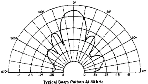
signal is limited to the type of surface the ECHO signal is reflected off of. Some surfaces provide good sonic reflections while others absorb sonic waves easily, limiting the operational range of the sonar rangefinder. Another negative aspect of sonar technology is that the signal sent is not a focused beam, but rather, a wide-angle beam that disperses in a large pattern. Figure 2.1 shows how a typical dispersed signal sent from a Polaroid

(16)

Typici Beam Patarn At s kHz

Figure 2.1 Dispersion Pattern for Polaroid Sonar

Polaroid, Inc. continues to manufacture ranging modules and ultrasonic transducers, the essential sonar components, even though their line of sonar cameras is out-of-date. The newest version of the ranging module is the 6500 Series Sonar Ranging Module (Part #615077). It is used in conjunction with the Polaroid high voltage electrostatic transducer to send and receive acoustic signals modulated by the ranging module and controlled by external sources, typically a computer or a microcontroller.

The 6500 series ranging module from Polaroid is the standard model used for sonar rangefinding. Some of the module's useful features include:

e accurate sonar ranging from 6" to 35 ft. (dependent upon the operating conditions) e operates on a single supply source in the range of 4.5 - 6.8 volts

* accurate clock output using a 420 kHz ceramic resonator (2.38 gs output resolution)

" variable data sampling rate

The ultrasonic ranging module is operated by controlling two signals, INIT and

BINH, and reading one signal, ECHO. INIT is the initializing signal which tells the

ranging module to start sending a ping. INIT will remain a high signal for the entire length of the maximum desired distance. BINH is a the blanking inhibit controller signal. The ranging module has an internal blanking inhibit time of 2.38 ms. ECHO is the signal

(17)

from the module indicates the length of time between the return signal and the end of the

INIT signal. It is from the difference in time of INIT and ECHO that the total time of

sound travel, At, is determined.

In actual operation, there is a series of 16 pulses that is sent to the electrostatic transducer after an INIT signal is received. The pulses are modulated at 49.4 kHz with a 400 volt amplitude that excites the transducer to generate an acoustic sound wave. After the pulses are sent, a 200 volt bias will remain on the transducer as the transducer waits for the return echo from the traveling sound waves. During a pulse cycle, a maximum current draw of 2 Amp can be expected.

To eliminate the ringing of the transducer from being detected as a return signal during a pulse, a pre-selected blanking inhibit time of 2.38 ms is automatically selected

by the ranging module. The blanking inhibit time in actuality is the time between the INIT signal going high and when ECHO can go high. This places a minimum on the

distance that can be detected. This blanking inhibit time can be adjusted by feeding a

BINH signal to the transducer. The BINH signal goes high after a the INIT goes high

and remains high for as long as INIT remains high. The difference in total time between INIT and BINH is the blanking inhibit time.

The purpose of a microcontroller is to provide the necessary signals to drive the ranging modules and measure the signal output, which is a function of the actual distance measured. The process is initiated when a signal is fed into the ranging board to initialize a 'ping', the term used to indicate a pulse of modulated sound. Once initialized, the ranging board automatically sends the ping and waits for a return 'echo', a term used to indicate the reception of the modulated sound. During this process, the micro controller measures the elapsed time between a ping and an echo. This interval is a direct function of the distance traveled by the modulated sound wave at the speed of sound in air. The speed of sound in air is:

V, r = ₍₁₎

where y is the ratio of specific heats(cp/c,) for air (= 1.4), R is the gas constant for air

(287.1 J/kg-K) , and T is the temperature in Kelvin.

The limited range, 30 ft. maximum range at optimal operating conditions and -15 ft. at nominal conditions, of sonar rangefinders are well suited for indoor and close range

(18)

operations. However, outdoor usage is limited by the constraints imposed by the limits of sonar technology. Ranges on ultrasonic sonars are determined by timing the time of flight of the ultrasonic sonic pulse between the time you send the pulse (ECHO) and when you receive a signal return (RECV). Figure 2.2 shows a diagram of an ultrasonic sonar. The time of flight (TOF) between the ECHO and RECV indicates the total flight time of the ultrasonic pulse. Distance is determined by the Equation 2:

1

d =-vxTOF

2 (2)

d = distance

v = velocity of travelling signal TOF = time of flight

Electrostatic Transducer

_Sonar Modulated Sound Wave s Object/

Micro Controller -.. Ranging ' Solid

Module : @Surface

1/2

Figure 2.2 A Typical Sonar Setup

ECHF 2

R ECV

TOF

(19)

A source of error in computing this distance is the temperature difference between

different operating environments. The temperature variance between a hot day and a cold day can be as high as fifty degrees Fahrenheit. This error can be estimated by:

Cerror = yiRT - VyRT2 (3)

where Ti and T2 are the different temperatures of the 2 operating environments. Given a variance of fifty degrees (1000 F for hot and 500 F for cold), this error would be 16.2 m/s. Thus, temperature should be a parameter or variable that can be changed based on the actual operating temperature of the sonar.

Distance resolution is limited by the timing resolution of whichever method is used to time the TOF signal. It has been determined over time however that anything better than %" resolution is unrealistic because of random noise and errors. Microcontrollers such as the Microchip's PIC microprocessor and Parallax's BASIC stamp are typical controllers used to control the signals and for timing of the sonar rangefinder.

(20)

2.2 Ultra Wide Band High Frequency Radar

One of the uses UWB technology is radar systems, permitting the precise measurement of distances, the detection of objects within a defined range of distances, or high resolution imaging of objects that are behind or under other surfaces. When combined with appropriate modulation techniques, UWB devices also may be used for communications purposes, such as the transmission of voice, control signals, and data. Most of the current equipment designs that have been investigated contain high level, distinct spectral lines concentrated near the center of the emission. However, it is recognized that, as the technology advances, this type of modulation is capable of spreading the signal levels over such a wide bandwidth that the emissions would appear to be similar to background noise. For such systems, the amount of energy appearing in any particular band should be extremely low. Such signals are not easily detected or intercepted.

Recently, there have been many advances in the development of UWB technology. UWB systems typically use extremely narrow pulse (impulse) modulation or swept frequency modulation which employs a fast sweep over a wide bandwidth. Because of the type of modulation involved, the emission bandwidths of UWB devices generally exceed one gigahertz and may exceed ten gigahertz. In some cases, these pulses do not modulate a carrier but instead, the radio frequency emissions generated by the pulses are applied to an antenna. The resonant frequency determines the center frequency of the radiated emission. The bandwidth characteristics of the antenna will act as a low-pass filter, further affecting the shape of the radiated signal. UWB pulse widths currently are on the order of 0.1-2.0 nanoseconds or even less. The emission spectrum appears as a fundamental lobe with adjacent side lobes that can decrease slowly in amplitude.

Applications for radar systems are currently being developed to detect buried objects such as plastic gas pipes or hidden flaws in airport runways or highways. Other radar systems could be used as fluid level sensors in difficult-to-measure situations such as oil refinery tanks and other storage tanks. Public safety personnel have expressed a desire for radar systems that can detect people hidden behind walls or covered in debris, such as from an earthquake. Other public safety personnel also have expressed a need for

(21)

UWB communications systems that can operate covertly. These possible communications systems could also be employed by heavy industrial manufacturers to overcome problems such as multi-path and machinery-generated radio noise.

Currently, two general types of UWB systems have been presented to the public, radar systems and communications systems that can be used for voice, data and control signals. These communication products are comparable to spread spectrum modulated communication systems. Like spread spectrum systems, UWB systems are able to employ gain processing on the received signal and can operate in the presence of high-powered transmission systems without considerable interference. UWB systems also may have a very low potential, relative to the total peak powers employed, for causing harmful interference to other users of the spectrum if the transmitted signal is spread over a wide bandwidth which may result in a relatively low spectral power density.

For the purpose of this thesis, there are two UWB systems that were considered. One is produced by Multispectral Solutions, Inc. and the other is a Micro Impulse Radar (MIR) developed by Lawrence Livermore National Laboratory. MSSI is recognized as an industry leader in the development of low probability of intercept and detection (LPI/D) communications and radar systems utilizing ultra wideband or short pulse technology. MSSI design experience includes GHz bandwidth RF as well as high-speed digital processing systems.

(22)

2.2.1 Multispectral Solutions, Inc.

Multispectral Solutions has been developing a miniature ultra wideband radar to demonstrate the ability to detect suspended wires and other small obstacles exceeding several hundred feet using a UWB sensor that uses an average output power of less than

10 microwatts. The sensor utilizes a short pulse waveform of approximately 2.5 nanoseconds in duration while the receiver uses advance processing technology to detect the radar return pulse and achieve range resolutions of less than one foot.

The key advantages of a Multispectral's UWB radar sensor include: e Wide volumetric pattern coverage

" Precise range control.

" High resolution, independent of range " Automatic system calibration

" Lower power requirements

* Low Cost

At the heart of the ultra wideband radar is the receiver/processor board which contains the high speed pulse detect, digital signal processor for 1/0 and range

calculations, and a field programmable gate array (FPGA). The MSSI UWB radar

utilizes a 1 watt, 400 Mhz instantaneous bandwidth pulse (2.5 ns pulsewidth) and a 10 Kpps pulse repetition frequency. Thus, the duty cycle is 0.0025% and the average power is 25 microwatts.

(23)

Wideband Patch Antennas

BPF Impulse Trigger

Source Source

Figure 2.5 Multispectral UWB Radar System Block Diagram2

T.m.l Dod.

Dec "rcWny _{Boot Row}

BM Ram

Contl Electonics

FPGA ftP EI.ctromcs

Figure 2.6 Multispectral UWB Radar System2

In summary, the primary advantages of the of a low power UWB radar include: * Extremely low probability of intercept and detection

* High anti-jam immunity

* Frequency diversity with minimal hardware modifications * Low cost components and assembly

Specifications:

Weight: 3 lbs.

Size: 150 cubic inches Power: 10+ Watt

(24)

4M __ -

-Freq 1.500GHz Span I.OGHz

RevBW 10MHz VidBW 7M2 SWP 20mS

LEVEL PiANB Freq te.5000MZ

ON= a ww I NWPA iUkt*,w.1t 97

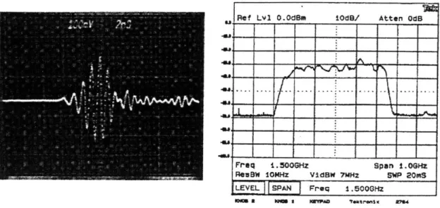
Figure 2.7 Measured Time and Frequency Response of Multispectral UWB Radar3

3 Courtesy of Multispectral Solutions Inc.

(25)

2.2.2 Micropower Impulse Radar by Lawrence Livermore National Laboratory

The Micropower Impulse Radar (MIR) is a fundamentally different type of radar that was invented and patented by Lawrence Livermore National Laboratory (LLNL). It is a pulsed radar like other ultra-wideband radars, but it emits much shorter pulses than most and, because it is built out of a small number of common electronic components, it is compact and inexpensive.

MIR technology has become one of LLNL's biggest technology transfer activity. They have licenses signed with industry in the areas of automobile back-up systems and in hand-held tools for finding studs and other objects behind walls. Many other diverse applications that are under investigation include fluid level sensing (electronic dipsticks), heart monitoring for medical applications, security systems, detection of breathing through walls or rubble (e.g., finding survivors of earthquakes), monitoring of infants for the possible prevention of Sudden Infant Death Syndrome (SIDS), underground and through-wall imaging, as well as many others.

One unique feature of the MIR is the pulse generation circuitry, which, while small and inexpensive, had never before been considered in radar applications. Each pulse is less than a billionth of a second and each MIR emits about two million of these pulses per second. Actual pulse repetition rates are coded with random noise to reduce the possibility of interference from other radars, while each is "tuned" to itself. The same pulse is used for transmitting to send via the transmit as for sampling the received signal.

Three direct advantages of the short pulse-widths are:

1. With pulses so short, the MIR operates across a wider band of frequencies than a

conventional radar, giving high resolution and accuracy, but also making it less susceptible to interference from other radars.

2. Since current is only drawn during this short pulse time and the pulses are infrequent, there are extremely low power requirements. One type of MIR unit can operate for years on a single AA battery.

(26)

3. The microwaves emitted by the pulse are at exceedingly low, and therefore medically

safe, levels (microwatts). Indeed, the MIR emits less than one-millionth the energy of a cellular telephone.

As with conventional radars, the antenna configuration on the MIR determines much of its operating characteristics. Several antenna systems have been designed to match the ultra-wide frequency characteristics of the MIR sensor. For the standard MIR motion sensor with a center frequency of about 2 GHz, LLNL use a small 1.5-inch antenna. However, the MIR is also flexible enough that it can operate at a relatively lower center frequency, using larger antenna systems, giving it longer range and better capability for penetrating water, ice, and mud.

What makes the MIR- so useful for security applications is its range gating capability. Imagine that each radio pulse is a large wave traveling across a lake. The wave bounces off an island and comes back to you. The amount of time it takes the wave to return depends on the distance to the island. By setting the radar's "gate," or echo acceptance range, to open only at the right time to receive echoes from a certain distance, it can ignore all other echoes. Range gating can therefore be used to set up an invisible security bubble around the radar. In a burglar alarm, for instance, the range might be set at 20 feet. The radar then detects only objects that modulate the reflected signal at this distance. It detects motion by repeatedly checking the echo pattern to see whether it changes over time; a change means the bubble has been penetrated by a moving object. This eliminates triggering on stationary background objects or "clutter."

The current MIR motion sensor can be fully concealed behind walls or inside drawers while detecting intruders at ranges up to 20 feet. Its sharply-bounded detection range is easily adjusted for any situation. In addition, the MIR can project a set or sweep of range shells to generate a filled volume of sensitivity. It does not respond to objects outside the current range gate, and it attempts to avoid false triggering on near objects such as insects. However, the range-gating mechanism may be susceptible to triggering on large-object movement in the near-field (inside the range bubble) because radar phenomena like multiple scattering will modulate the range-gate return.

(27)

Averaging of many thousands of pulses is done on th.e MIR to reduce the effects of noise and to increase sensitivity. A single received pulse in the nanosecond time scale may be contaminated with various forms of outside interference, but if the returns of many pulses at the same range gate are combined, the result is much more representative of the actual return. The number of averages per range gate is adjustable (nominally it is about 10,000 samples) and is one of the tradeoffs in the MIR design.

The exact pulse emission and detection times are randomized for three reasons:

1. Continuous wave (CW) interference, such as from radio and TV station harmonics,

may cause beat frequencies with the received echoes that can trigger false alarms. When the 10,000 samples of MIR return echoes are averaged at randomly-dithered times, random samples of CW interference are effectively averaged to zero.

2. Random operation also means that multiple MIR units can be collocated without interfering with each other. Channel allocations are not needed and a nearly unlimited number of sensors can be in the same vicinity even though they occupy the same wideband spectrum.

3. Randomizing also spreads the sensor's emission spectrum to the point that it resembles

random thermal noise, making it difficult to distinguish from background noise. That is, this randomizing makes the MIR very stealthy.

Figure 2.8 MIR Motion Sensor4

(28)

The MIR UWB motion sensing system projects an invisible "bubble" at the motion-sensing boundary that has a sharply define, adjustable radius. Intrusion into the bubble indicates motion via a non-microphonic, non-Doppler process that can also measure velocity.

Figure 2.9 MIR Modular Rangefinder5

The MIR modular rangefinder is a compact, low-cost ultra-wideband radar with a swept range gate. The device generates an equivalent-time A-scan (echo amplitude vs range, similar to a WWII radar) with a typical range sweep of 4 inches to 10 feet and an incremental range resolution, as limited by noise, of .01 inch.

2.2.2.1 Potential Applications

Uses include replacement of ultrasound rangefinders for fluid level sensing (a dipstick without the stick), vehicle height sensing, and robotics control. When positioned over a highway lane, it can collect vehicle count, vehicle profile, and approximate speed data for traffic control. An FCC Part 15 compliant version transmits RF packets rather than a short impulse, and can provide swept-range quadrature Doppler information. A major application for this microradar is imaging. It operates in spectral regions that readily penetrate walls, control panels, and to an acceptable extent, concrete and human tissue.

(29)

The basic antennas have a very broad beamwidth and corresponding low gain. They are suitable for synthetic beam imaging where broad illumination is desirable. Narrower beamwidths and higher gain can be obtained on a broadband basis with horns, reflectors or dielectric lenses.

Unfortunately, MIR technology is still new and is not yet readily available on the market for testing and evaluation. In general, UWB technology is too new for practical use and general understanding. The technology is fairly complicated and the signal processing of UWB seems to play a very important role in determining the use and limits of the technology.

(30)

2.3 Laser Rangefinding

Lasers are becoming more common for use as rangefinding sensors because their

prices have dropped significantly over the years. Not only is pricing a major

consideration but performance is as well. Laser rangefinding provides highly accurate and fast range readings because the pulses can be focused and travels at the speed of light

(-3.Ox108 m/s). Relative to sonar rangefinding, laser rangefinding offers significant advantages in speed, accuracy, and resolution. In both cases, distance is determined by similar methods, by measuring the time between when a signal is sent and when it's received. Unfortunately, since the speed is light is difficult to measure, resolution in laser rangefinding is limited by the method used to measure the TOF.

Similar to ultrasonic sonar rangefinding, laser rangefinding have constraints as well. It is limited not only by the signal strength of the laser pulse output but also, the reflectivity of the surface of the object. In extreme cases, a perfect reflective material such as mirror will make it difficult if not impossible to get a return laser signal and on the other side, a perfect black body surface will completely absorb the laser signal. After all, a laser signal is a form of light. There are various types of reflections that can occur; diffuse (Fig. 2.10), mirror-like (Fig. 2.11), and retro-reflection (Fig. 2.12).

(31)

incident beam

diffusely r efle ctin g

target target surface

Figure 2.10 Diffuse reflections6

glossy or mirnor-like

target surface

target

Figure 2.11 Mirror-like reflections6

ReTroreflecting foil or cat's eyes reflector

Figure 2.12 Retroreflections6

(32)

For different objects and surfaces, the amount of laser light returned is characterized by the reflection coefficient p. For diffuse reflecting surfaces, the maximum theoretical value for p is 100%. For mirror-like or retroflecting surfaces, the maximum theoretical value for p can exceed 100%. Table 1 shows the reflection coefficient of various surfaces for a 900 nm wavelength signal.

Material Reflective Coefficient p

White Paper Up to 100% Lumber 94% Snow 80-90% Beer Foam 88% White Masonry 85% Clay Limestone Up to 75% Newspaper . 69% Tissue Paper 60% Deciduous Trees 60% Coniferous Trees 30%

Carbonate Dry Sand 57%

Carbonate Wet Sand 41%

Beach Sands 50%

Rough Wood Pallet 25%

Concrete, Smooth 24%

Pebble Asphalt 17%

Lava 8%

Black Neoprene 5%

Black Rubber Tire Wall 2%

Reflecting Foil 3M2000X 1250%

Opaque White Plastic 110%

Opaque Black Plastic 17%

Clear Plastic 50%

Table 1: Material Reflectivity7

To boost the return signal strength of a laser, extremely powerful laser pulses are used and fired in small time increments. The average power maybe equivalent to that of a weak laser but the signal to noise ratio on the receiver is increased by a factor of 10's,

100's, or 1000's. This is the method commonly used, thus, it is call pulsed laser

rangefinding. The average power is calculated by the following Equation 4:

(33)

P = (Peak - Power) x freq x p - width (4)

P = Average Power

PeakPower = Maximum Power of Laser

Freq = Laser Pulse Repetition Frequency (samples/second) p-width = Pulse width length (second)

Laser rangefinding has traditionally been a very difficult process. Because light travels at a speed of 3.Ox 108 m/s, it became necessary for the laser rangefinding system to

have a timer capable of measuring time in nanosecond resolution. To time a 1

nanosecond differential signal, the minimum clock frequency required is 1 Gigahertz

( seconds), a very small fraction of a second. Over the years, technology has given us

109

the advantage of making timing circuits smaller and faster. In the 60's, laser rangefinders weighted in the tens of pounds. Today, they are lightweight and portable and weights

(34)

2.3.1 Laser Triangulation

Even a few years ago, laser rangefinding was generally thought of as being very hard to accomplished efficiently and effectively. People used techniques such as laser angle triangulation to effectively approximate range. This process was range limited and relatively poor in quality.

sin B sin A

b -a

A B

Laser positions

Figure 2.13 Triangulation Technique

Laser triangulation makes use of a technique that's been used thousands of years

by surveyors. It makes use of the law of sines to get a range. By knowing the two angles

of a triangle and their common side, the remaining sides can be calculated. In the particular case of rangefinding, corners A and C of Figure 2.13 represents two separate cameras or charged coupled devices (CCD). The common side is the baseline separation distance, c. Thus, range can be calculated by measuring angles A and B and using the equation:

sin A sin B

(35)

a =bsin A (6)

sin B

Also, since angle B can not be measure directly, it can be calculated from angles A and C from the following equation:

a~b sinA (7)

sin(ir - A-C)

This type of laser rangefinding is typically classified as passive laser rangefinding. Amazing, it technique also represents how the human eyes work and how people estimate distances. Each eye works as a detector and range is internally calculated or estimated in our heads.

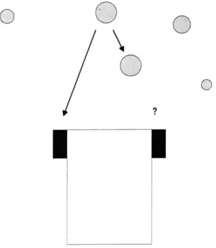
Unfortunately, passive laser rangefinding systems have self-imposed limits. Besides being dependent on two separate sensors, each individual sensor needs to view the target source directly, otherwise, triangulation will not be possible. This is illustrated in Figure 8. Another major problem with triangular rangefinding is that range and resolution is limited by the resolution of the receiver in determining angular return signals. Because of this, triangulation systems are mainly effective at close range only.

0i

0

(36)

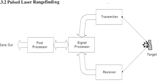
2.3.2 Pulsed Laser Rangefindi ng

Data Out _{DataOutProcessor} _Processor-

-Target

Receiver ''

Figure 2.15 Pulsed Laser System

Pulsed laser rangefinding is the dominant type of rangefinding technique used today. Pulsed laser rangefinding works on a very basic principle, the distance to the target object is directly proportional to the time of the return ECHO. Similar to sonar rangefinding, laser rangefinding operates on the same technique. A source signal is propagated and a return signal is received. The time between the two signals is directly proportional to distance traveled. There are inherent advantages to using a laser rangefinder compared to a sonar rangefinder. Sound travels at a speed of approximately

1 ft/s at room temperature while light travels at approximately 1 ft/ns, about a million times faster.

One difficulty for laser detection is because the EM signals travel so fast, high speed electronics are required to detect reasonable distances. This is typically not a problem for conventional radar systems that may have ranges in the kilometers, but for short-range applications, this imposes requirement for short-range applications.

In a pulsed laser system, the emitted pulse has a rather large amplitude that is characterized by a pulse width, the carrier frequency, and sometimes even the modulation of each pulse. Optimally, it is ideal to have an extremely large amplitude and short pulse width. A large laser signal amplitude will increase the signal-to-noise ratio of the return

(37)

signal thereby, increasing the probability of detection and range. A small pulse width translate to lower average power for the laser making it more eye safe and less power hungry.

Modulation of a pulsed laser system only occurs when it requires separating the laser signal from the background noise such as ambient light. In this case, the laser is pulsed and modulated at a particular frequency and the receiver carries a band-pass filter that only allows signals of a particular frequency through. Although this is rarely used in typical rangefinding applications, it is possible to use this to carry "information". By changing the modulation frequency, it is possible to encode information in the laser signal and decoded on the receiving end.

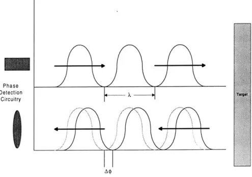
2.3.3 Continuous Wave Phase Shift Rangefinding

The final method in laser rangefinding is rangefinding using a continuous wave phase shift. Although similar to the TOF methods, instead of sending a short and distinct pulse, a continuous modulated signal is emitted. Rather than timing signals directly like in the TOF method, the continuous wave method measures the phase difference between the emitted and detected signals.

Similar to the TOF method, the elapsed time of a CW wave is related to range by:

At=- (8)

C

d = distance c = speed of light

Figure 2.16 illustrates the transformation between time and frequency domains of a continuous wave phase shift. The elapsed time of the phase difference between the emitted and detected signal is normalized by the period of the wave. This is shown in Equation 9. At Ap ₍₉₎ T 27c 1 T = wave period = -A$ = phase shift

(38)

f = modulation frequency

By combining Equations 8 & 9, the range can be expressed as:

d =c=A AA (10)

f

-4r 4r

Thus, by modulating the laser at a known frequency

f

and measuring the phase shift $, this method can yield a range of distance d.

For example, if a continuous laser source is modulated at 10 Mhz, each period of the wave is 100 ns. In terms of the speed of light, this cycle is equivalent to approximately 100 ft in length per wave period. If an object is 50 ft way, the equivalent round trip travel time for wave is 100 ft, thus, there will be zero phase difference. However, if the target object is closer than 50 ft and the phase difference is measurable, the range can be determined easily from the phase difference using Equation 10.

One of the major problems with CW wave laser rangefinding is the ambiguity in the calculated ranges. In the previous example where the CW wave is modulated at 10 Mhz, ranges can differ by multiples of 50 ft. Thus, if there was an object at 50 ft, 100 ft,

150 ft, etc, the CW wave method would not be able to distinguish from the various ranges

from looking purely at the phase difference.

Phase Detection

Circuitry

A / '

(39)

In comparison, CW laser rangefinding systems offer some important advantages compared to the TOF method. The first reason is because of their continuous nature, this makes for very fast operations. There is no need to fire a pulse and wait for the return. The second advantage is, there is no need to measure time absolutely to determine range and resolution but only the relative phase difference. The range and resolution is determined by the modulation frequency and the resolution of the electronics in determining the phase difference between the outgoing and incoming laser signals. This actually lessons the requirements on the electronics compared to TOF ranging methods in addition to allowing ranging operations at extremely close ranges.

The three primary types of methods for laser rangefinding, triangulation, time-of-flight, and CW each has their advantages and disadvantages. Technology has advanced enough over the years that now, people can purchase off the shelf parts components to do rangefinding and there are firms out there that sells and specializes in the various

components of a laser rangefinder. Of the three techniques, the TOF method is

seemingly the most dominant because in theory and practice, it is the least complicated to understand and easiest to use. There are specific manufacturers for the various pulsed lasers, receivers, and even timing circuit. Also, laser rangefinding has become such a hot and profitable area in the recent years that many companies are making their own packaged rangefinding systems. Most of these firms are proprietary which imposes limits on engineers and scientists to learn more about the system custom build one that fits their specific needs.

(40)

2.3.4 Various Packaged Laser Rangefinding Systems

There are many packaged laser rangefinding systems on the market today. These packages include OEM modules, packaged single point solutions, and 2D scanning solutions. The following will contain examples of existing systems on the market today.

2.3.4.1 LEICA LRF OEM Laser R angefinder Modules

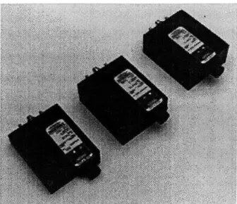
These rangefinder modules are available as basic assemblies, integrated with optics and housing. A typical example of the integrated form is the LEICA MRF2000. Basic assemblies can be manufactured in different configurations with the following main features:

LEICA LRF LEICA LRF

Wavelength 860nm 1550nm

Eye-safety class ANSI 2136.1 EN60825-1 (1994)

(1993)

AMa&)mum range 3300m 50M

Distance accuracy _{+1 to 2m} _{+1 to 2m} (1 ~ ~ ~ ___ + to) 2m__ :Measurement rate 15per minutef20prmnt Data transmission RS232 or 422 RS232 or 422

ower supply _DC0-28 _{6 V DC, 10-28 V DC} DC

AConsumption 400 mA/6 V 450 mA/6 V

Weight 95g 100g

Implemented in MRF2000 VECTOR

Figure 2.17 Leica OEM Comparison Table

Figure 2.18 LEICA MRF2000 Monocular rangefinder (L) and standalone unit (R)8

(41)

2.3.4.2 Riegl Laser Distance Sens or LD90-3GF

The distance and level meter LD90-3-GF with glass-fiber coupled optical head makes use of the time-of-flight method to determine the distance of a remote target by measuring the transit-time between transmission and reception of a short laser pulse.

Distance measurements can be performed to both non-cooperative and cooperative targets with high accuracy, interference immunity, and excellent reliability. The serial interface allows communication and operation of the instrument. Furthermore, the LD90-3-GF can be equipped with the various digital and analog data outputs frequently used in industry. The measuring system consists of a lightweight and small optical head and a separate electronics box, connected by a duplex glass-fiber cable with connectors on both sides.

Specifications for Riegl Laser Distance Sensor LD90-3GF:

Measuring range (depending on the reflection coefficient of the target) Good, diffusely reflecting targets, reflectivity 3 80% up to 100 m Bad, diffusely reflecting targets, reflectivity 3 10% up to 35 m Reflecting foil 2) or plastic cat's-eye reflectors > 1000 m Minimum distance, typically 1 m

Distance measurement Accuracy: Typically ± 2cm, in the worst case 5cm Measuring time (ms or s): 1Oms/ 20ms/ 50ms/ 0.1/ 0.2/ 0.5/ 1/2

Statistical deviation (cm): ±7/ ±5/ ±3/ ±2/ ±1.5/1I/ ±0.7/ ±0.5

Resolution (cm)5): 5/ 5/ 2/ 2/ 1/ 1/ 0.5/ 0.5

Accuracy: ± 0.3 m/s

Measuring time, typically 0.5 s

Serial data interface RS232 or, alternatively, RS422

Baud rate selectable between 150 Bd and 19200 Bd, further 38.4 kBd and 115.2 kBd Physical Weight Data: Electronics: 1.5 kg & MK36 Head: 0.6 kg

Figure 2.19 Riegl Laser Distance Sensor LD90-3GF Head Unit w/o Electronics9

(42)

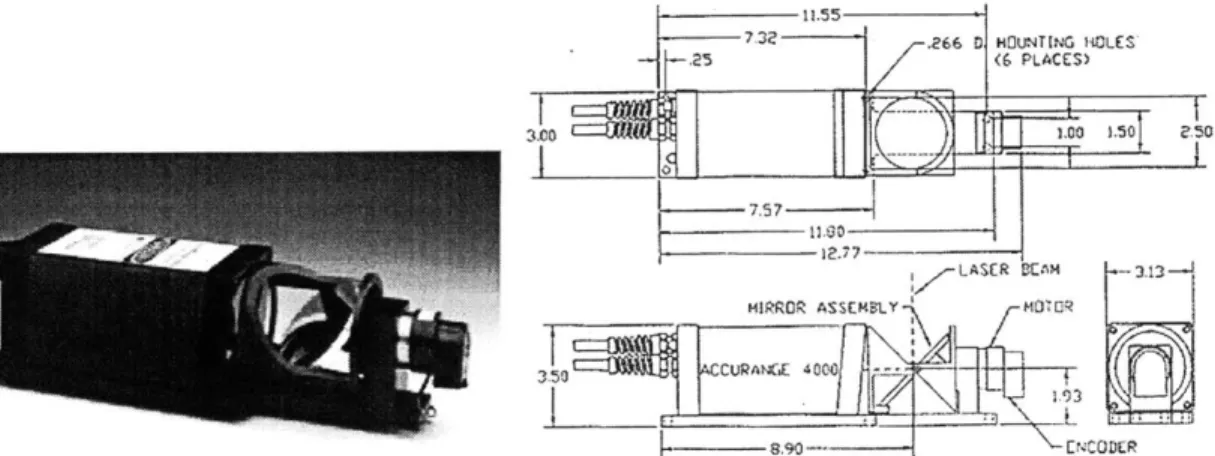
2.3.4.3 AccuRange 4000

The AccuRange 4000 is an optical distance measurement sensor with a useful range of zero to 50 feet for most diffuse reflective surfaces. It operates by emitting a collimated laser beam that is reflected from the target surface and collected by the sensor. The sensor is suitable for a wide variety of distance measurement applications that demand high accuracy and fast response times.

Specifications for Accurange 4000:

Zero to 50 feet operating range for most surfaces. 0.1 inch accuracy, 0.02 inch short-term

Optional RS-485/422, 4-20mA current loop, and pulse width outputs. RS-232 serial output standard.

Reflected signal amplitude output for greyscale images. Fast response time: 50KHz maximum sample rate. Lightweight, compact, low power design.

Tightly collimated output beam for small spot size

Two output beam configurations available: visible or infrared

Ideally suited to level and position measurement, machine vision, autonomous vehicle navigation, and 3D imaging applications.

Weight: 2.5 lbs. Power

Sensor Power: +5 Volts (+5V min, +6 V max) @ 400 mA

Heater Power: +5 Volts (+5V min, +6 V max) @ 4A, temperature dependent. May be used to stabilize sensor temperature in low-temperature environments

3,13

Weght: 22 oi- 91 Outer Shell Anodild Akuminum - 6.66

Mosarccu: Foura -32 400aded

mowiting bos

1.60

2.38

Figure 2.20 Accuity Research Accuirange 400010