HAL Id: inria-00107623
https://hal.inria.fr/inria-00107623
Submitted on 19 Oct 2006
HAL is a multi-disciplinary open access archive for the deposit and dissemination of sci-entific research documents, whether they are pub-lished or not. The documents may come from teaching and research institutions in France or abroad, or from public or private research centers.
L’archive ouverte pluridisciplinaire HAL, est destinée au dépôt et à la diffusion de documents scientifiques de niveau recherche, publiés ou non, émanant des établissements d’enseignement et de recherche français ou étrangers, des laboratoires publics ou privés.
Training and evaluation of the models for isolated
character recognition
Szilárd Vajda
To cite this version:
Szilárd Vajda. Training and evaluation of the models for isolated character recognition. [Contract] A02-R-481 || vajda02b, 2002. �inria-00107623�
EDF PROJECT
Multi-oriented and multi-size alphanumerical character
recognition
PART II.
Training and evaluation of the models for
isolated character recognition
This report corresponds to the task n.2 of the contract entitled: "Apprentissage et évaluation de classifieurs de caractères"
September 2002 – October 2002 Szilard VAJDA
READ Group
LORIA
1. Plan
• The developed system steps
• Test Results
• The future development
2. The developed system steps
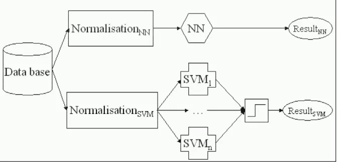
Figure 1 shows the different steps of the developed system. As we can see, there are two major alternatives:
• NN alternative: after a linear normalisation respectively the Goshtasby
transform, only one NN trained for all the classes determines the belonging class for the presented character.
• SVM alternative: here the Goshtasby transformation is used for the character
normalisation, then the input character is presented to each SVM trained for each class. At last, the SVM results are normalized and combined (integrated) in order to determine the final class.
Figure 1: Developed system flowchart 2.1.1. NN Normalisation
In that case we used two normalizations. The first one, it’s a classical linear normalisation. For each class, we perform the medium image size by this we mean to calculate the average width and height for all the images in the database, and then, for each character (image), the size is normalised in function of the mean height and width, calculated before. The second one is the Goshtasby transform which will be presented in detail in chapter 2.1.2.
2.1.2. SVM Normalisation
The multi-oriented aspect of the characters necessarily induces some confusion between classes having visual similarity. The literature mentions some methodologies more or less adapted to character shapes normalisation. We made the choice of the Ghoshtasby transformation, because of its simplicity, by giving an
image (shape matrix) rather than complicated features like Fourier transformation, higher order moments, etc.
The Goshtasby transformation gives for each character image a normalized shape matrix. For the shape matrix size, we used the mean image size of the whole database. This size is very important because it determines the finesse of the image shape sampling. Even though this normalisation which solves somehow the multi-orientation and the multi-size invariances, it has some drawbacks. In fact, it accentuates the similarity between some character shapes. These are the cases for classes like: (0, o, O, C, D, Q), (v, V, A), (I, i, l, 1), (z, Z), (s, S), (8, B), (6, 9, p, b), (x,X), (p, P), (u, U). These confusions are the side-effects of this transformation.
2.2. Model Training
2.2.1. NN Models
• The topology
We used an MLP (multi-layer perceptron) with two hidden layers. In the input layer we have 576 units (24*24, the size of the planar shape, which is the result of the Goshtasby transformation) and in the output layer we have 62 units, each corresponding to a specific alphanumerical character class. The used learning algorithm is the gradient back-propagation. Between the input layer and the first hidden layer, respectively between the first hidden layer and the second hidden layer, the units (neurons) are not fully connected, we are using a connection topology, by this we mean, we are using local connections, by having rectangular image portions which are connected, in order to have more local information. These rectangles are super-positioned each to other, be using a shift. Between the second hidden layer and the output layer the units are fully-connected, which mean that every unit from the second hidden layer is connected to each neuron in the output layer, in order to synthetize the local information coming from the previous layers.
• Training aspects
In the training phase, we can set a lot of parameters, concerning the neural networks. These parameters are: the size of the rectangle, which is responsible of the amount of local information. By increasing this value, we can add inside the network,
more local information. It can also fix, the learning rate, the value of η, which serves
to set the rapidity of the learning process (back-propagation algorithm), and in the mean time we have an internal step counter, to set the numbers of the presentation of each character from the database. The epoch (external step counter) is setting how many times we want to pass the whole database via the network. At each epoch (external step), we can save the actual state of the network, in order to have an idea, how it’s working the learning, by this we mean to follow the different steps of the learning process and to have the possibility to test the convergence of the gradient descent back-propagation algorithm which was used during the learning phase.
2.2.2. SVM Models
The SVMs are trained to perform pattern recognition between two classes by finding a decision surface determined by a subset of the complete training set, termed Support Vectors (SV).
Contrary to the NN, the SVM is just a binary classifier. As we pointed out, the drawback of the systems like the SVMs that is not possible to classify with them, N different, mutually-exclusive classes. In order to create a classifier, like the NN, with SMVs, we have to normalize and integrate the results.
The main idea of data normalization method, is to calculate an average distance (coming from the positive samples which where already learnt), for each SVM, each class, and to divide the real outputs (distances) of this SVM’s with these distances, in order to receive comparable outputs for the different SVMs.
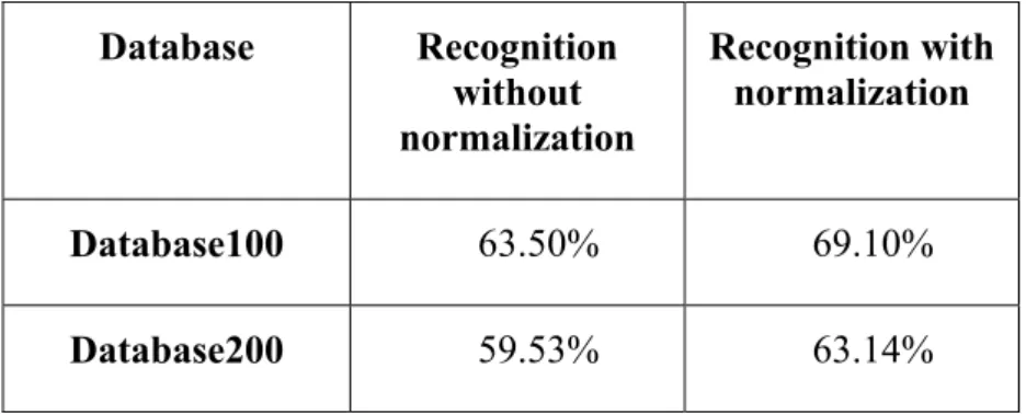
Below we show some results concerning the SVMs data point recognition, with and without normalization. Database Recognition without normalization Recognition with normalization Database100 63.50% 69.10% Database200 59.53% 63.14%
Table 1: SVM results without and with data normalization
Remark: By Database100 respectively Database200 we mean databases, in which we take in account just the first 100 respectively 200 samples from each represented class from the image database, which was presented in detail in Characterization and normalization of image database (EDF Project, PART I). In the cases when the number of samples in the classes were less than 100 or 200, we took the maximal number of samples from the given class.
• Training aspects
In the training process, we have to teach SVMs as many different classes we have. This mean, that the teaching process for the SVMs is 1-v-r (one versus rest). Here also we can set a lot of parameters, but we are using the parameters concerning the complexity and the error, for the convergence of the learning process, more exactly, for the precision of the classification.
3. Test Results
In the testing phase was not used any kind of rejection criteria so this mean that each object will be classified as an alphanumerical character (a-z,A-Z,0-9)
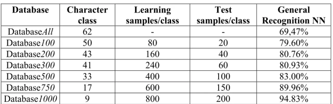
3.1. NN Results (Goshtasby tranform) Database Character class Learning samples/class Test samples/class General Recognition NN DatabaseAll 62 - - 69,47% Database100 50 80 20 79.60% Database200 43 160 40 80.76% Database300 41 240 60 80.93% Database500 33 400 100 83.00% Database750 17 600 150 89.96% Database1000 9 800 200 94.83%
Table 2: Results of the NN for the different databases
DatabaseAll information: Character class Recognition rate (NN) Confusion with Character class Recognition rate (NN) Confusion with 0 32.88 o 1 67.24 A 2 90.17 z 3 76.10 5 4 87.79 u 5 78.04 6 6 58.40 5 7 82.26 5 8 65.15 B 9 75.54 7 A 92.74 4 B 55.00 e C 71.60 c D 70.43 o E 78.25 6 F 87.23 r G 83.67 3 H 81.58 R I 43.52 l J 72.73 7 K 50.00 7 L 89.47 l M 83.00 H N 86.43 M O 43.30 o P 73.22 p Q 25.00 a R 77.93 p S 42.04 s T 89.85 1 U 90.62 u V 97.53 Y W 0.00 d X 82.35 x Y 42.86 V Z 40.00 2 a 69.71 8 b 89.13 d c 64.71 C d 84.62 J e 79.39 8 f 70.00 F g 21.05 9 h 52.17 F i 20.00 l j 20.00 l k 87.10 1 l 64.56 I m 53.03 E n 83.69 D o 62.25 O p 65.79 P q 0.00 1 r 65.19 T s 50.00 S t 67.18 l u 58.96 U v 29.17 V w 100.00 - x 93.99 T y 20.00 Y z 20.00 Z
As we can observe, concerning the confusion, the recognition rates for such kind of characters like (0, o, O), (s, S), (1, I, l, I, j), (v, Y) are not high, because this classes are confused very often with other classes and these confusions are coming from the property of size and rotation invariancy of the Goshtasby algorithm.
In the Table 4 we can find the results of the NN with the rough database, so without the position, scale and rotation invariant transformation (see Goshtasby), just using a simple size normalization presented in detail in chapter 2.1.1 and including also the junk class.
Database Character class General Recognition NN
DatabaseAll1 63 69,88%
DatabaseAll2 62 79.52%
DatabaseAll3 - 70.69%
DatabaseAll4 - 80.93%
Table 4: NN results with the linear normalization
The DatabaseAll1is the whole database and the junk class, DatabaseAll2 is the
whole database without the junk class, DatabaseAll3is the whole database with some
class regroupment and the junk class, and DatabaseAll4is the whole database with
some class regroupment without the junk class. By regroupment we mean to treat as one, character pairs like: (0, o, O, D), (s, S), (p, P), (1, I, l, I), (c, C), (x, X)
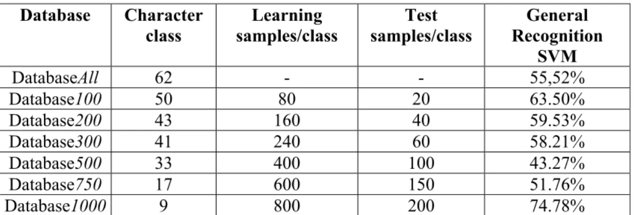
By making the regroupment, it’s true, we are loosing information, but we win in the score, and in the after treatment part, we can use specific verifiers, in order to separate the classes which were regrouped, which technique is often used to solve these kind of problems. 3.2. SVM Results Database Character class Learning samples/class Test samples/class General Recognition SVM DatabaseAll 62 - - 55,52% Database100 50 80 20 63.50% Database200 43 160 40 59.53% Database300 41 240 60 58.21% Database500 33 400 100 43.27% Database750 17 600 150 51.76% Database1000 9 800 200 74.78%
Table 5: SVM results for different databases
DatabaseAll information: Character class Recognition rate (SVM) Character class Recognition rate (SVM) 0 35.73 1 54.31 2 67.92 3 58.46 4 75.00 5 51.69 6 35.20 7 58.87
8 51.52 9 47.48 A 72.65 B 40.00 C 53.09 D 64.35 E 61.86 F 56.03 G 44.90 H 52.63 I 44.44 J 45.45 K 25.00 L 82.11 M 59.00 N 75.00 O 27.84 P 57.92 Q 0.00 R 61.26 S 45.22 T 72.08 U 67.19 V 83.95 W 0.00 X 70.59 Y 71.43 Z 0.00 a 55.43 b 47.83 c 47.53 d 57.69 e 53.44 f 20.00 g 5.26 h 26.09 i 31.76 j 0.00 k 77.42 l 45.57 m 37.88 n 68.79 o 56.29 p 34.21 q 0.00 r 48.15 s 39.84 t 41.98 u 43.28 v 29.17 w 0.00 x 74.86 y 0.00 z 20.00
Table 6: SVM results for each character class
In the cumulative table, we can find the general recognition rates for the SVMs respectively the NNs for the same databases.
Database Character class Learning samples/class Test samples/class General Recognition NN General Recognition SVM DatabaseAll 62 - - 69.47% 55.52% Database100 50 80 20 79.60% 63.50% Database200 43 160 40 80.76% 59.53% Database300 41 240 60 80.93% 58.21% Database500 33 400 100 83.00% 43.27% Database750 17 600 150 89.96% 51.76% Database1000 9 800 200 94.83% 74.78%
Table 7: Result comparision for NN and SVMs
The red is more present than the blue one, so this is mean, that the NN is giving better results than the SVM. The cause of this low recognition rate in the SMVs case can be explained with the high number of classes and the number of samples in each class. In the next few tables we are presenting the confusion matrices of the NN respectively SVM for DatabaseAll.
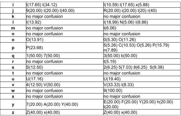
We took in consideration just the classes where the confusion is at least 5% SVM case, respectively 10% NN case, in order to have a real vision of the confusions.
DatabaseAll (NN & SVM case)
Character class
Major confusion (≥10%) in NN
case Major confusion (≥5%) in SVM case
0 D(10.79) O(16.63) o(24.69) A(7.94) o(13.90)
1 no major confusion t(5.39)
2 no major confusion no major confusion
3 no major confusion 8(5.51)
4 no major confusion no major confusion
5 no major confusion S(8.78)
6 no major confusion 5(5.60)
7 no major confusion no major confusion
8 B(11.36) B(8.33) a(5.30)
9 no major confusion 8(9.35)
A no major confusion no major confusion
B 8(10.00) e(14.00) 8(13.00) H(5.00) a(5.00) e(6.00)
C c(20.99) C(16.67)
D no major confusion no major confusion
E no major confusion 6(5.08)
F no major confusion P(6.38)
G no major confusion 0(8.16) a(6.12)
H no major confusion M(13.16) R(5.26)
I l(37.04) i(9.26) l(28.70)
J no major confusion d(9.09)
K 7(25.00) k(25.00) S(25.00) i(25.00) m(25.00)
L no major confusion no major confusion
M no major confusion no major confusion
N no major confusion no major confusion
O o(41.24) 0(17.53) D(7.22) a(5.15) o(22.68)
P no major confusion P(9.84)
Q a(25.00) n(25.00) u(25.00) 2(25.00) a(50.00) u(25.00)
R no major confusion no major confusion
S s(29.94) 3(7.64) 5(6.37) s(7.64)
T no major confusion no major confusion
U no major confusion u(15.62)
V no major confusion no major confusion
W d(100.00) C(100.00)
X x(17.65) R(5.88) S(5.88) x(17.65)
Y M(14.29) V(42.86) E(14.29) v(14.29)
Z 2(20.00) M(20.00) z(20.00) 6(20.00) l(40.00) t(20.00) x(20.00)
a no major confusion B(6.29)
b no major confusion O(6.52) h(6.52) u (6.52)
c C(10.29) C(20.59)
d no major confusion no major confusion
e no major confusion no major confusion
f F(20.00) A(5.00) F(35.00) I(5.00) L(5.00) Y(5.00)
Y(5.00) e(10.00) i(5.00) r(5.00) t(5.00) g 9(31.58) c(10.53)
5(5.26) 6(5.26) 9(21.05) A(5.26) D(10.53) E(5.26) K(5.26) P(5.26) V(5.26) o(5.26) p(5.26) q(5.26)
i I(17.65) l(34.12) I(10.59) l(17.65) x(5.88) j 9(20.00) I(20.00) l(40.00) R(20.00) i(20.00) l(20) r(40)
k no major confusion no major confusion
l I(13.92) I(18.99) N(5.06) I(8.86)
m no major confusion t(6.06)
n no major confusion no major confusion
o O(13.91) 0(5.30) O(11.26) p P(23.68) 5(5.26) C(10.53) O(5.26) P(15.79) n(7.89) q 1(50.00) 7(50.00) 3(50.00) b(50.00) r no major confusion t(5.19) s S(12.50) 2(6.25) 5(7.03) 8(6.25) S(9.38)
t no major confusion no major confusion
u U(17.16) U(19.40)
v 4(12.50) V(50.00) V(33.33) l(8.33)
w no major confusion 9(100.00)
x no major confusion no major confusion
y 7(20.00) A(20.00) Y(40.00) E(20.00) F(20.00) Y(20.00) h(20.00) l(20.00)
z Z(40.00) x(40.00) Z(40.00) x(40.00)
Table 8: Confusion for the NN ans SVMs in recognition
The confusions can be placed in two categories. In the first one, we can find the confusion which are the side effect of the Goshtasby transformation, presented before and some transformation, which seems to be illogical like: m confused with t, K confused with 7, Q confused with u & n, etc. For this we have 3 explanations:
1) the labelling process is not sufficiently correct, by this we mean that the extracted characters, from their nature after the segmentation can induce some errors/confusions in the labelling manipulation
2) the images are bad
3) some characters are low represented in the database 3.3. Conclusions
3.3.1. Concerning the Goshtasby’s transformation
The implementation is quite simple and it doesn’t need extra memory or computer power. This mean, that for images, used by us, the transformation could be performed in real time. Apparently the “distances” between the different classes is enough, but the transformation is not able to distinguish classes like (0, o, O, C, D, Q), (v, V, A), (I, i, l, 1), (z, Z), (s, S), (8, B), (6, 9, p, b), (p, P). In that cases, the differences (distances) are minimal.
Taking in consideration the results of the NN obtained with the brute database, using just a little size transformation, we can appoint that the Goshtasby transformation it is not so efficient, but it could be if we are refining the shapes, after the transformation by using a shift technique.
3.3.2. Concerning the neural networks results
As we can see, by growing the number of samples, the results get higher and higher. Taking a look in the literature, this model can give good results, so we think
than the database it is not sufficiently correct, and for this kind of images, we should add some contextual information (orientation, angle, etc.)
3.3.3. Concerning the support vector machines results
As the results are showing us, the recognition rates are not sufficiently good. The possible raisons could be that the SVMs learning algorithm is not converging or we should act more in data results normalization/integration, more specifically in the normalization of the distances of the different SVMs, because the problem is, for each character we will receive a distance from the different SVMs, trained to make distinctions between the different classes, and these distances can not be compared, because they are coming from different models, which can not be measured with the same measurement.
Another aspect is the data integration process, where at the moment we are using a function (argmax, the maximal distance given by the different SVMs for the character which is in the recognition process) which could be replaced with a neural network, which has the capability to find this function itself, by learning. This technique is often used in the literature. The second method is more general than the first one.
3.3.4. Concerning the confusions in the recognition process in NN case
The results are showing us than when we are increasing the number of examples in the different classes, the confusion from the same classes is decreasing or stop, but we have some cases when this confusion is going higher. These variation of the confusions between classes can be explained by the growing number of the examples from the different character classes and also with the decreasing number of the classes. In Database100 we have 50 classes, in Database500 we have just 33 classes.
3.3.5. Concerning the confusions in the recognition process in SVM case
The results are showing use, than when we are increasing the number of samples in the classes, the confusion rate is going higher and higher. This elevation of confusion can be explained with the number of examples. As we know, the SVMs are giving good results when the number of classes and the number of samples in the classes is not so high.
3.3.6. Concerning the whole system
Taking in consideration the recognition results, the confusions of the two systems, NN respectively SVM, and the confusion which are caused by the Goshtasby’s transformation, we should regroup some character classes, like (8, B), (p, P), (z, Z), (0, o, O, D), (1, l, i, I), (s, S), (k, K) etc., and by this technique we can raise the results, and after that we can use some specially trained networks or SVMs to make the differences between characters which have the same shape matrix, otherwise speaking, treated as one class before.
4. Perspectives
Concerning the Goshtasby transformation, we are looking for a shifting method, which can redress the images in a sense of the angle. This shifting method will be used to benchmark the images against some representative images which will be collected manually from the database. For each character class we will define some model images, and we will try to redress the other images from the same class to these model images.
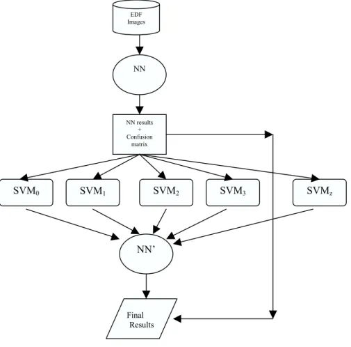
Taking in consideration the results of the NN and SVM we are working already in the combination of these two systems, in order to increase the recognition results. We are developing a combination scheme, combining the NN model with the SVM in order to raise the recognition score. The flowchart of the combination is presented hereinafter:
Figure 2: Combination of the NN model with the SVMs model
In the next few lines, I would like to make some comments, in order to understand the reasoning of this combination scheme, presented in Erreur ! Source du renvoi introuvable. EDF Images SVM0 NN results + Confusion matrix NN SVM1 SVM2 SVM3 SVMz NN’ Final Results
Taking in account the results of the NN respectively SVMs, we can affirm than the recognition property of the NN is better in the cases when we have “enough” samples, and the SVMs results get higher when the number of samples is slow.
So, in the first phase, we would like to use an NN, in order to place (to separate) the image object into one presumed class or another. In cases, when we are certainly sure, that the NN prediction is good, we can stop the recognition process. When we have the results of the NN, we are also looking for the confusion matrix, in order to see, which other candidates could be also taken in consideration. By having the first p classes (the classes which the character presumed by the NN could be also confused), we passing the results of the NN by these p possible SVMs, trained to recognize these classes. (Remark: Taking a look to the confusion matrix (NN case) we can notice two things. At each character class we can find some classes with a high confusion score and a lot of classes with minimal confusion score, which can be ignored. So we think that is sufficiently enough to pass the images through just the first p SVMs, where the confusion it’s really measurable). This parameter will be a global parameter of the combination model.
The results of the SVMs are passed via a second NN, which is not so complex, architecturally speaking, and the final results will be given by this NN’.
We are using this NN’ for the reason to find the best possible function, which will give the final result.
In the NN’ case we could also taking in account the credibility of each SVMs, in order to help the NN’ classifier to decide for the best solution.
This function could be also defined by us manually (at the moment argmax), but it’s better to use an NN for this mechanism to approximate this function with a good precision.
By having already the results of the NN and the SVMs, for the different classes, right now we are working on the second NN’ in order to estimate the first results of the proposed combination model.