Hydration of drug-like molecules with molecular density functional theory and the hybrid-4th-dimension Monte Carlo approach

In these works, as the potential asso- ciated to each protein structure results from an average over the degrees of freedom, the kinetics is guided by transition rates between

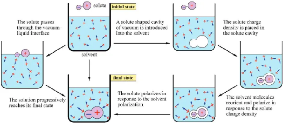
Solvent equilibrium structure, polarization and beyond Equation 1 states that at the same time as MDFT produces the solvation free energy of arbitrarily complex molecule (the value

Since Mellies has shown that (a calculus of explicit substitutions) does not preserve the strong normalization of the -reduction, it became a challenge to nd a calculus satisfying

Standard deviations of the time series of estimated free energies, with implicit solvent, explicit solvent using screened potentials, and explicit solvent using softcored

Adsorption energy E ads as a function of vertical distance d for PTCDA on Cu(111), Ag(111) and Au(111) employing the DFT þ vdW surf method.. The distance d is evaluated with respect

Intraprotein interactions and many-body dispersion effects We start out by investigating the Fip35-WW trajectory by artificially removing the surrounding solvent from a

The difficulty here is that we need to verify all the execution traces in order to certify a security protocol when R is not ground confluent (definition of strong inductive

In Section IV, we give and discuss the results, including the optimiza- tion of the parameters µ and λ on small sets of atom- ization energies (AE6 set) and reaction barrier