A computational model for multistage axial compressor design

(1)

A

COMPUTATIONAL MODEL FOR MULTISTAGE AXIAL COMPRESSOR DESIGN

by

ARNAUD IRVING WISNIA

Ingenieur Civil Electricien et Mecanicien, Universith Libre de Bruxelles, 1994 Licencid es Sciences Physiques, Universite Libre de Bruxelles, 1994

Ingenieur de l'Aronautique, Ecole Nationale Sup6rieure de l'Aeronautique et de l'Espace, 1996

Submitted to the Department of Aeronautics and Astronautics in partial fulfillment of the requirements for the degree of

MASTER OF SCIENCE at the

MASSACHUSETTS INSTITUTE OF TECHNOLOGY February 1998

©

A,/

Author

[~-

Department of Aeronautics and Astronautics January 12, 1998

T, ,V g.

Dr. Choon S. Tan Principal Research Engineer Thesis Supervisor

Accepted by

ThsKLC

Professor Jaime Peraire Associate Professor of Aeronautics and Astronautics Chair, Graduate Office

mA

')9ig~

-L'

Certified by

(2)

(3)

A

COMPUTATIONAL MODEL FOR MULTISTAGE AXIAL COMPRESSOR DESIGN

by

ARNAUD IRVING WISNIA

Submitted to the Department of Aeronautics and Astronautics on January 12, 1998, in partial fulfillment of the

requirements for the degree of Master of Science

(4)

ABSTRACT

A framework is developed to perform multistage compressor computations, with the objective of assessing the impact of blade-row interaction involving wakes and end-wall flow on compressor performance. This framework consists of analyzing the flow in a discrete blade row or a stage, embedded in a multistage environment where the other blade rows are modeled by distributed body forces and heat sources. This ensures proper impedance matching of the flow upstream and downstream of the considered discrete blade row or stage.

A blade row model is first developed in steady flow, then adapted to the unsteady flow environment. Three different classes of model elements are shown to have dif-ferent roles: heat sources model the flow entropy rise, the streamwise body force components model the blade row work input on the flow, and the orthogonal body force components model the flow turning and pressure rise. The model is assessed in steady flow by comparing, on a momentum- and energy-average basis, the flow in a discrete blade row with the flow obtained when the blade row is replaced by its model. In two dimensions, the equivalence of the two flows is shown analytically. In three dimensions, three relevant test cases are used: a straight duct, a stator, and a rotor. All aerodynamic and thermodynamic flow variables of interest are observed to be well matched on an average basis by the model. The only discrepancy in the stator and rotor test cases is shown to be the result of the model's inability to account for the blade thickness distribution, which can be included via a blockage factor.

The model is then assessed in unsteady flow by comparing the flow in a discrete blade row with the flow obtained when the blade row is replaced by its model, in terms of time-averaged pressure rise and loss. In a first test case, unsteadiness is generated by a wake model at the inflow of a stator. The stator is then replaced by its blade row model. Discrepancies in the time-averaged static pressure rise and loss measured in the two flows are shown to result from the absence of wake-boundary layer interaction phenomena in the model. A second test case is run with a rotor-stator stage, and the flow in the stage is compared with the flow obtained when the stator is replaced by the model. The time-averaged static pressure rise and loss in the rotor are observed to be identical in the two cases. A discrepancy in the stator time-averaged static pressure rise and loss is once again attributed to the lack of wake-boundary layer interaction in the model. Overall, the replacement of the stator by the model cuts down the computation time by a factor of 3 to 4.

Based on the results obtained here, the proposed framework can potentially be used to analyze the impact of flow phenomena in a multistage environment on compressor

performance and design.

Thesis Supervisor: Dr. Choon S. Tan Title: Principal Research Engineer

(5)

ACKNOWLEDGMENTS

Coming to MIT was a milestone in my professional life, and I would like to thank my parents, Kelman and France Wisnia, my sister Audrey, and my girlfriend Vanessa, for their encouragement to take on this challenge, and their continuous support and love throughout my stay here. I could not have done it without you.

I am profoundly indebted to my advisor, Dr. Choon S. Tan, whom I wish to thank for offering me the chance to work with him on this project. His constant support, friendly comments, constructive critique and vision have played a major part in the achievement of this work. I have learned enormously from his constant strive for improvement and excellence, and will benefit from it over the longer term, whichever path I follow in my professional endeavors.

I would like to express my gratitude to Professor Edward M. Greitzer for his continuous support in this project, and for helping me discovering new and challenging paths of investigation by constantly asking the right questions.

During the course of my work, I benefited enormously from the input of several visiting Professors. The discussions I had with Professors Frank E. Marble and Nick A. Cumpsty proved an invaluable source of advice and new ideas. I would particularly like to thank Professor William N. Dawes, for his time and help in solving some of the most challenging CFD problems encountered here.

The Gas Turbine Laboratory at MIT is a large, wonderful community, and I couldn't possibly cite here all of my fellow students and the staff members whose continuous help and support made my experience at MIT much more than academic. I particularly wish to thank Ken and Yifang for their valuable input at our research group meetings, Amit and Sonia, for their help in using the software. To Leo, Ahmed, Luc, Amit, Rory, Adam, Chris, Omar, Jinwoo, Zolti, Jonathan, Sanith, John, and all the GTLers, thank you, I had a great time here thanks to you all. I would also like to thank Bill Ames and the GTL golf fans for a number of great outings... even though

(6)

we might not have always played very well !

This work was supported by a Fellowship of the Belgian American Educational Foundation, a Fulbright Scholarship from the Commission for Educational Exchange between the United States, Belgium and Luxemburg, and a grant from Mitsubishi Heavy Industries, Takasago Research Center with Dr. Sunao Aoki and Dr. Yutaka Kawata as technical monitors. Their support is gratefully acknowledged.

(7)

6.2 Figures of Merit for the Model in Unsteady Flow . . . . 6.2.1 Rotor-Stator Interaction Affecting the Stator . . . 6.2.2 Rotor-Stator Interaction Affecting the Rotor . . . 6.3 Numerical Validation of the Unsteady Blade Row Model 6.3.1 Overview of the Test Cases ... 6.3.2 Measurement Points and Averaging Planes . . . . 6.3.3 Test Case Number 1 ... 6.3.4 Test Case Number 2 ... 6.3.5 Test Case Number 3 ... 6.4 Summary: Unsteady Model Effectiveness . . . . 7 Summary and Conclusions, Recommendations for 7.1 Summary and Conclusion . . . . 7.2 Recommendations for Future Work . . . . . . . . . 120 . . . . . 121 . . . . . 121 . . . . . 122 . . . 122 . . . . . 127 . . . 130 . . . 144 . . . 150 . . . . . 163 Future Work

A Overview of the NEWT Computational Fluid Dynamics package A.1 The M esh Generator ...

A.1.1 General Considerations ...

A.1.2 General Structure of the Mesh . . . . A.1.3 Addressing of the Mesh Nodes . . . . A.1.4 Properties of the Mesh ...

A.1.5 Input Data to the Mesh Generator . . . . A.2 The Flow Solver and Turbulence Model . . . .

A.2.1 Flow Equations ... . ... ...

165 165 167 169 169 169 170 170 172 172 173 173 6.1

(10)

A.2.2 Resolution Procedure ... 174 B Implementation of the Body Force and Heat Source Model

B.1 Creation of the Model Geometry . . . . B.2 Creation of the Model Geometry Mesh . . . . B.3 Computation of the Model Elements . . . . B.3.1 Computation of the Model Body Forces . . . . B.3.2 Computation of the Model Heat Sources . . . . B.3.3 Computation of the Model Body Forces Streamwise Co B.4 Implementation of the Model in the NEWT Code . . . . B.5 Comparison of the Real and Model Flows . . . .

mponent

C Wake Model

C.1 Boundary Conditions in the NEWT Code . . . . C.2 The Concept of Wake Modeling . . . . C.3 W ake Primary Variables ...

C.3.1 Relative Stagnation Pressure . . . . C.3.2 Relative Stagnation Temperature . . . . C.3.3 Relative Tangential Flow Angle . . . . C.4 Construction of the Model ...

C.4.1 Choice of a Relative Stagnation Pressure Profile . . . . C.4.2 Computation of Pitchwisely Nonuniform Stator Inflow

Bound-ary Conditions . . . . C.5 Estimation of the Wake Model Parameters . . . . C.5.1 Relative Flow Angle . . . .

C.5.2 Relative Stagnation Temperature T2 . . . .

C.5.3 Relative Stagnation Pressure P/2 (9) ... Bibliography 177 178 178 179 181 197 200 201 204 207 207 208 209 209 210 211 212 212 213 215 216 216 216 219

(11)

LIST OF FIGURES

1-1 M ixing plane . . . 23

1-2 Methodology for Multistage Compressor Computations ... 25

2-1 Computation mesh for a stator blade row with turbulence model . . . 34

2-2 Computation mesh for a stator blade row with viscosity modeling . . 36

2-3 Computation mesh for a stator blade row with blade modeling . . . . 37

2-4 Stator model embedded between two rotors . ... 43

3-1 Typical Control Volume in a Blade Row . ... 48

3-2 Typical Velocity Vector and Body Force in the Model Flow ... 60

3-3 Different levels of Blade passage Discretization . ... 65

4-1 Discretization of a 2-D stator blade row . ... 72

4-2 2-D control cell . ... . .. .. .. ... . .. . . . . .. .. . . .. . 73

5-1 Straight Duct Test Case: Real and Model Computational Meshes . . 84

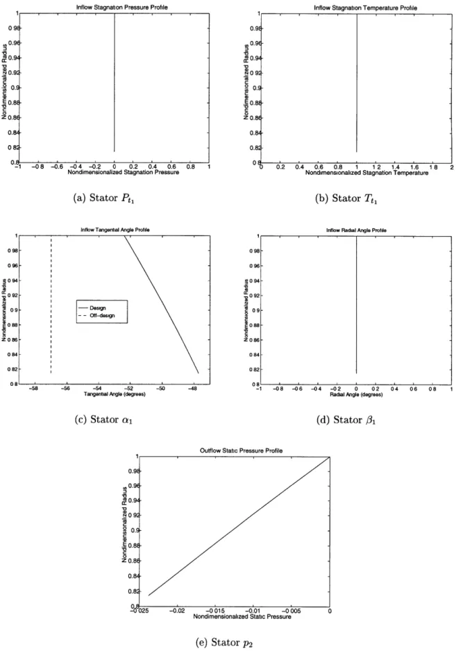
5-2 Stator and Rotor Test Cases: Real and Model Computational Meshes 86 5-3 Stator Test Case Boundary Conditions . ... 88

5-4 Rotor Test Case Boundary Conditions . ... 89

5-5 Real/Model Flow Comparison in Duct Test Case . ... 92

5-6 Real/Model Flow Comparison in Stator Test Case at Design .... . 95

5-7 Real/Model Flow Comparison in Stator Test Case Off Design . . .. 96

5-8 Comparison of Areareatlow and PUmodef low vs. x for stator test case . . 97

Areamodelflow _{PUreal flow} 5-9 Radially-integrated Body Force Components in Stator Test Case at Design ... 98

(12)

5-10 Impact of the Solver Artificial Viscosity of Real/Model Flow

Stagna-tion Pressure Comparison ... 100

5-11 Real/Model Flow Comparison in Rotor Test Case in Relative Frame . 102 5-12 Real/Model Flow Comparison in Rotor Test Case in Absolute Frame 103 5-13 Real/Model Flow Stagnation Temperature Comparison in Stator Test Case at Design - Zoom ... 105

5-14 Impact of the change of a heat source on the overall flow entropy dis-tribution . . . .. . 106

5-15 Real/Model Flow Comparison in Stator Test Case at Design after Two Iterations . . . 110

6-1 Unsteady Boundary Conditions at Stator Inflow . ... 117

6-2 Radially-integrated Body Force and Heat Source Components - Quasi-Steady M odel . . . 118

6-3 Location of Measurement Points in Unsteady Flow . ... 128

6-4 Location of Averaging Planes in Rotor in Unsteady Flow ... . 129

6-5 Location of Averaging Planes in Stator in Unsteady Flow ... . 130

6-6 Unsteady Real and Model Geometry Meshes . ... 131

6-7 Instantaneous Entropy Visualization at Mid-Span in Real Geometry . 133 6-8 Time-Averaged Stator Inflow Boundary Conditions . ... 135

6-9 Instantaneous Entropy Visualization at Mid-Span in Model Geometry 137 6-10 Average Static Pressure and Entropy - Comparison of the Real and Model Geometries - Detail ... 139

6-11 Real/Model Flow Comparison in Steady Flow - Static Pressure and Entropy . . . ... 141

6-12 Typical Profile of S3.5rea(0) - Sstator wake(O) vs. 0 . . . . 143

6-13 Transformation of Real Geometry Mesh for Mixed-Out Inflow Compu-tations . . . .. . 145

6-14 Average Static Pressure and Entropy - Comparison of the Real and M odel Geom etries ... 147

(13)

6-15 Comparison of Rotor-Stator and Rotor-Model Computation Meshes . 152

6-16 Rotor-Stator Computation Convergence Curves . ... 153

6-17 Flow Entropy Visualization at Midspan in Rotor-Stator Configuration 154 6-18 Rotor-Model Computation Convergence Curves . ... 156

6-19 Flow Entropy Visualization at Midspan in Rotor-Model Configuration 158 6-20 Average Static Pressure and Entropy - Rotor-Stator Geometry . . . . 159

6-21 Average Static Pressure and Entropy - Rotor-Model Geometry . . .. 160

6-22 Time Traces of Rotor Backpressure at Six Relevant Locations . . . . 162

A-1 Structure of a Typical NEWT Mesh . ... 171

B-1 Construction of the Model Geometry . ... 179

B-2 Model Flow Geometry Structured and Unstructured Meshes .... . 180

B-3 Typical Model Geometry Mesh Cell . ... 180

B-4 Typical Constant x Integration Surface . ... 186

B-5 Typical Constant x Real Geometry Mesh Face . ... 186

B-6 Typical Constant r Integration Surface . ... 190

B-7 Typical Constant r Real Geometry Mesh Face . ... 191

B-8 Typical Periodic Boundary Model Geometry Mesh Face ... 195

B-9 Model geometry structured and unstructured 2D meshes ... . 203

C-1 Fitting of the relative stagnation pressure profile ... . . . 212

(14)

(15)

LIST OF TABLES

2.1 Irrotational Flow Behavior in Stator Blade Row . ... 39

2.2 Rotational Flow Behavior in Stator Blade Row and Subsequent Model Requirem ents .. ... . ... ... ... . . . .. . . . . .. . ... . 42

5.1 Duct Test Case Real Flow Mesh Geometrical Data . ... 83

5.2 Duct Test Case Model Flow Mesh Geometrical Data . ... 83

5.3 Duct Test Case Boundary Conditions . ... 85

5.4 Stator and Rotor Test Cases Mesh Geometrical Data . ... 87

5.5 Stator Test Case Artificial Viscosity Parameters . ... 99

6.1 Unsteady flow phenomena captured by different levels of model com-plexity ... 120

6.2 Stator pressure rise and loss when wakes proceed through, compared to the case when wakes are mixed upstream . ... 126

6.3 Unsteady Computations Mesh Geometrical Data . ... 130

(16)

(17)

NOMENCLATURE

Roman

A surface

A1 surface in contact with fluid A2 surface in contact with solid

a speed of sound (V RT)

C, static pressure coefficient CPt stagnation pressure coefficient

CP constant pressure specific heat of air, 1005 J/(kg.K)

E internal energy

Sbodyforce per unit mass

centrifugal force per unit mass

Fc Coriolis force per unit mass

H enthalpy

I rothalpy

L length of 2D mesh face

M Mach number (v)

rh mass-flow

Nblade number of blades on a blade row

surface normalized outside pointing normal vector

p pressure

Pt stagnation pressure

(18)

Q

heat

R perfect gas constant of air, 287 J/(kg.K)

Re Reynolds number r radial coordinate S entropy s curvilinear coordinate t time T temperature T stagnation temperature

u x-component of the velocity

v y-component of the velocity

V volume

absolute velocity vector relative velocity vector

x axial coordinate

y y-coordinate in a cartesian reference frame vector coordinate of a point in the blade passage

Greek

a tangential angle

/ radial angle

' Ratio of specific heats

6 deviation angle

A thermal conductivity

p dynamic viscosity

Sonabla ( a- + -fY + t)

(19)

(D heat source power per unit volume

p density

0stress tensor

viscous stress tensor

X7 x-component of viscous friction T7 y-component of viscous friction

0 tangential coordinate

Subscripts

cv control volume

hub blade row hub

in, inflow blade row inflow plane

irrev irreversible

lam laminar

mg model geometry

nd nondimensional

out, out

flowblade

row outflow plane

II

component parallel to the local velocity vector I component orthogonal to the local velocity vector

r radial component

ref reference value

rg real geometry

t stagnation (or total) fluid quantity

T turbulent

tip blade row casing

0 tangential component

(20)

y y-component in a cartesian frame of reference

z z-component in a cartesian frame of reference

Superscripts

weak average value model flow value

weak average of model flow value relative frame of reference

Other useful notations

CFD computational fluid dynamics

1D one-dimensional (x)

2D two-dimensional (x and 0)

(21)

CHAPTER

1 INTRODUCTION

1.1 Evolution in Compressor Design Methods

High performance compressors have been the object of innumerous research efforts since World War II, when the development of the first jet engines opened a wide new scope of applications for them. Design methodologies have also dramatically changed. Initial designs were relying on 1D meanline analyses coupled with cascade data, and most often involved numerous iterations between design and testing until a satisfactory configuration was found. Radial Equilibrium and Streamline Curvature methods [3], [25] brought the analytical design from one to two dimensions, and led to improved first bench test performance. Such methods have enabled the designers to reduce the number of design iterations.

With the computer era, new perspectives have appeared in compressor design with the development of Computational Fluid Dynamics, and modern design methods rely on computational results rather than testing [20]. The benchmark today is to do a full 3D computer design and achieve the expected performance at the first bench test [19].

The exponential increase in computing power witnessed in the last ten years has enabled the computation of the turbulent flow in complex 3D geometries. Such

(22)

com-putations, applied to single blade rows or single stages, have led to sharply reduced compressor design time cycles, and have helped develop creative ideas for blade de-signs leading to substantial performance improvements [20]. In spite of this, at the scale of an entire multistage compressor, a full 3D viscous computation of the flow still remains a daunting prospect, and is not yet achievable in amounts of time acceptable for design purposes without massive parallel computing [19].

1.2 Motivation of the Research

As direct multistage computations cannot be used for multistage compressor designs, some kind of approximation must be done. One of the most commonly used approx-imations is the mixing plane approach [24], [13], in which each blade row is designed individually (figure 1-1). This leads to an essentially steady design method, and does not reflect the impact of any unsteady phenomenon on the compressor performance. However, it has long been known that the unsteady interaction between neighbor-ing blade rows has an important role in determinneighbor-ing the maximum pressure rise and efficiency of a compressor. Smith [26] showed on the single-stage General Electric Low-Speed Research Compressor that a one-point efficiency gain and a two-to-four point pressure rise increase could be achieved by reducing the axial gap between the blade rows from 37% to 7% of the stator axial chord. Similar results were found by Mikolajczak [22], whereas Hetherington and Moritz [16] achieved a 2-point efficiency gain by increasing the spacing in front of the rotor blade rows in a multistage com-pressor. Gostelow [14] also showed the existence of an optimal blade row spacing for turbines.

In addition to blade row spacing, other design parameters such as blade loading and spanwise loading distribution are known to have a major impact on performance, much of which cannot be accurately predicted without taking into account unsteady interaction phenomena.

(23)

Stage downstream boundary conditions

Mixed-out stator

inlet boundary conditions

z

Mixed-out rotor outlet boundary conditions

Figure 1-1: Mixing plane approach to the design of a single stage. The rotor is first designed, using as outflow boundary conditions a first guess of the conditions upstream of the stator. The rotor outflow is then used as the inflow boundary condition for the stator design.

Several mechanisms of blade row interaction, and their impact on performance, have been studied in the past. A review of these mechanisms is provided by Valkov [28]. Blade row interaction manifests itself in two forms: potential and vortical. Potential interaction is the impact of the blade row pressure field on the upstream and downstream blade rows. Vortical interaction encompasses the effect of vortical structures - wake, tip vortex, streamwise and corner vortices - on downstream blade rows. Both forms have been shown, analytically and experimentally, to impact efficiency and pressure rise.

Even though these mechanisms have been studied in the past, this has only been Stage upstream

(24)

done at the scale of a single stage. This is because, as already pointed out above, it is unrealistic to perform multistage 3D computations with currently available computa-tional resources. The ability to implement multistage computations would provide:

* for the researcher, a means to assess on a qualitative and quantitative basis the flow interaction effects within the multi-blade row environment that impact stage matching and compressor performance,

* for the design engineer, a tool to improve multistage compressor designs by taking into account unsteady interaction phenomena in a rigorous manner.

The objective of this research is to develop and implement an innovative method-ology for performing multistage compressor computations, with the goal of reducing the computation time to affordable levels.

1.3 Statement of the Problem

When designing a blade row embedded in a multistage compressor, the flow in the whole multistage compressor must be computed at once if the unsteady interaction effects are to be accounted for, even though most of the flow details in the other blade rows do not need to be known. This leads to a considerable waste of computation power.

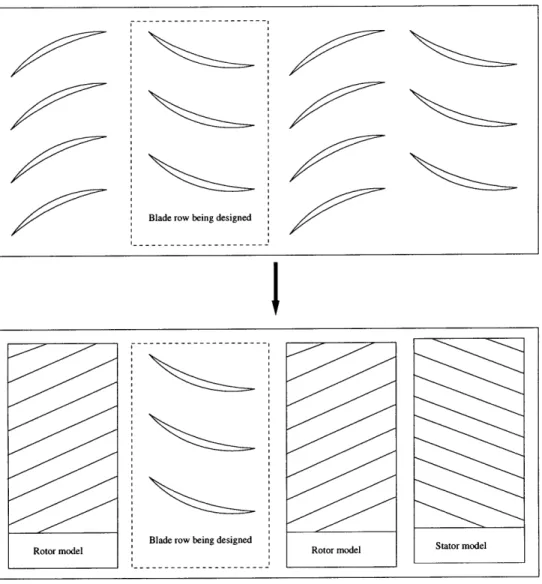
The methodology developed here consists of replacing the blade rows for which the flow details are not needed on a blade-to-blade level but only on an averaged basis by a computationally economical model (figure 1-2). The model must be designed to be computationally economical while duplicating the important interaction phenomena. This new methodology is developed on a step-by-step basis. Modeling is first addressed for a single blade row in steady flow in order to understand the key concepts. This model is then adapted to the unsteady flow environment and tested in a rotor-stator configuration. Multistage applications will be the object of upcoming research

(25)

I I I _I I _I I I I I I I I I I I \\ _I' I I I _I I Blade row being designed :

Figure 1-2: Methodology for Multistage Compressor Computations

efforts.

In the course of this work, a number of questions are addressed:

* What constitutes a model in Fluid Dynamics? What are the physical properties that models can duplicate? What level of modeling is adequate to reach the goal stated here?

* What should be required of a model in steady flow? Given the geometry of a blade row and its operating point, how can a steady model be created? How well are the model requirements met? What can be done to improve the model?

(26)

* What are the model requirements in unsteady flow? How well does the steady model developed above satisfy the unsteady flow requirements? Is there any improvement from using a quasi-steady model rather than a steady one? What can be done to further improve the model?

* Are most or all physical effects which impact blade row performance in a multi-blade row environment well accounted for by the model? If not, does it explain the results observed when testing the model in unsteady flow? In regard of this, can such a model be used effectively in a multistage compressor?

1.4 Contributions of the Thesis

1.4.1 Modeling in Turbomachinery Fluid Dynamics

The framework developed here consists of computing the flow in a discrete blade row or a stage, embedded in a multistage environment where the other blade rows are modeled by distributed body forces and heat sources. It provides a means of addressing the flow phenomena that impact compressor performance and design in multistage environment.

Present Work in the Context of Previously Published Work

The concept of using body force distributions to represent a blade row is not new. It has been used by Marble [21], Horlock and Marsh [18], Denton [11] and Adamczyk [1] among others.

Marble has developed an axisymmetric body force model for throughflow compu-tations in blade rows. This body force can be seen as the distribution of the force applied by the blade on the flow, which can be decomposed into a normal pressure force and a tangential shear force. Marble's model can be computed if the blade geometry and various flow variables at the blade surface are known.

(27)

Horlock and Marsh showed, by averaging the 2D differential form of the continu-ity and momentum equations across a blade passage, that 2D blade rows in steady inviscid flow can be replaced by distributed body forces. The computation of their body forces requires the knowledge of the static pressure on the blade surface.

Denton used distributed streamwise body forces to simulate viscous effects in a flow otherwise computed using an inviscid solver. He showed that the pitchwise profile of body forces can be arbitrarily chosen, provided they create the correct shear force at the blade surface, which is therefore the input in the construction of his model.

Finally, Adamczyk showed by applying three averaging operators on the 3D un-steady Navier-Stokes equations that, among other things, unsteadiness resulting from a multi-blade row environment can be captured on an averaged basis by a steady computation using distributed body forces, heat sources and deterministic stresses. The model elements are obtained by the application of a closure model, in the same way as a turbulence model is used to obtain Reynolds stresses in a turbulent flow computation.

In this thesis, the steady flow in the blade row for which the model is sought is first computed, using an existing CFD code. The discrete blade passage is then discretized in a number of control volumes, and the equations of fluid mechanics and thermo-dynamics are written in their integral form on each of these control volumes. The model elements, body forces and heat sources, are extracted from the implementation of these integral equations on the computed flow. Such a model can, in principle, be computed for a set of operating points in the blade row or stage pressure character-istic, yielding a model which can respond to flow nonuniformities and design changes in a multistage environment. The modeling approach used here is clearly different from previously published work.

The model developed here has been designed for completeness, i.e. to model both the aerodynamics and thermodynamics of the flow, and for flexibility, so that the same modeling approach can be applied to construct a model representation that ranges

(28)

from a simple, zero-dimensional actuator disc to a fully three-dimensional unsteady model.

A New Breakdown of Model Elements

Model elements are shown to belong to three distinctive categories: streamwise com-ponents of the body force vectors, orthogonal comcom-ponents of the body force vectors, and heat sources. The role that model elements of each category have in modeling a blade row, and the flow variables that they impact in the model flow, are explained on a physical basis. The heat sources are shown to model the flow entropy rise, the

streamwise components of the body forces the blade row work input on the flow, and

the orthogonal body force components the flow turning and pressure rise.

Equivalence of the Model Flow and the Discrete Blade Row Flow

A first-of-a-kind analysis is developed to show that, in 2D flow cases, the replacement of a blade row by its model will duplicate the aerodynamic and thermodynamic flow variables on an averaged basis.

1.4.2 Expected Contribution to On-Going and Future

Re-search Efforts

The implementation of the model developed in this research leads to computational codes which are expected to be used in the course of on-going and future research efforts:

* A code has been written, and a methodology has been defined, to compute the model elements for any given blade row geometry at any given operating point. This code offers flexibility in its ability to include the relevant physical effects as needed.

(29)

* Two CFD codes, the steady and unsteady versions of the NEWT code developed by Dawes, have been adapted so that one or several blade rows can be replaced by the model developed here.

1.5 Organization of the Thesis

The concept of modeling in Fluid Dynamics is introduced in chapter 2. A physi-cal approach is used in order to understand what level of modeling is required to accomplish the objectives of this research.

The equations of Fluid Dynamics and Thermodynamics are used in Chapter 3 to explain how a model can be created for a given blade row at a given operating point, and how it relates to the physics of the flow. In Chapter 4, an analytical study shows the effectiveness of the model for 2D steady cases, whereas test cases are presented in Chapter 5 to assess the model performance in 3D steady cases. A brief description of the CFD mesh generator and solver used in this research is provided in appendix A. The numerical implementation of the model is detailed in Appendix B.

In Chapter 6, the model derived for steady flows in Chapters 3 through 5 is as-sessed in an unsteady flow environment. Unsteadiness is first generated by nonuniform inflow boundary conditions moving relative to the blade row, representing hypothet-ical incoming wakes. The derivation of the wake model is detailed in Appendix C. Time-resolved and time-averaged flow variables help understand qualitatively and quantitatively if and how the model reproduces the physical phenomena known to affect time-averaged performance in a multistage compressor. A further investigation of the model performance in unsteady flow is then conducted in a realistic multi-blade row environment. The model replaces a stator located downstream of a discrete rotor, and time-resolved as well as time-averaged flow data shows how realistic nonunifor-mities such as real wakes and tip vortices are processed by the model, and how the influence of the stator model on the upstream rotor compares with the influence of the discrete stator in the rotor-stator configuration.

(30)

Finally, conclusions on the overall performance of the model are presented in Chapter 7, and guidelines are provided for future work. Expectations on the usefulness of such a model in multistage computations are stated.

(31)

CHAPTER

2 MODELING IN TURBOMACHINERY

COMPUTATIONAL FLUID DYNAMICS:

KEY CONCEPTS

As pointed out in Chapter 1, a blade row model is necessary if multistage compressor computations are to be conducted using acceptable computational resources. The main reason for which multistage turbomachinery computations are so highly time-consuming is the presence of many different length scales. This concept will be explained below, and will be the basis for the development of a model.

2.1 Parametric Dependence of Computation Power

on Problem Length Scales

When a mesh is constructed for flow computation, the spacing between mesh points must be small compared to the length scale of all the phenomena to be described. The grid resolution is therefore dictated by the length scale of the smallest phenomenon of interest. On the other end of the scale, the largest length scale of the problem deter-mines the overall size of the mesh. The larger the ratio of the largest to the smallest

length scales, the more mesh points are needed, the more computation-intensive each iteration will be.

(32)

In CFD1 codes using explicit resolution schemes, such as the code used in this re-search, the smallest length scale of the problem also has a great impact on the number of iterations needed to complete the computation. Indeed, for stability purposes, the time step used when running a CFD code is limited, and the limit is directly pro-portional to the smallest length scale of interest [17]. The presence of small length scales in the problem therefore not only makes each iteration more computationally intensive, as explained in the previous paragraph, but also requires a smaller time step, and hence more iterations to reach convergence.

Airflows in compressors have almost always high Reynolds numbers, and are there-fore turbulent. The smallest length scale is then the size of the boundary layer turbu-lent structures, some of them only a few percent of the boundary layer thickness. It is important to capture these structures when computing the flow in a compressor, as they impact the shear and heat transfer at the wall. On the other hand, the largest length scale in a multistage compressor is the overall size of the machine, which can be several orders of magnitude larger than the length scale of the turbulent flow struc-tures. The ratio of the largest to the smallest length scales is therefore huge, and the computing resources required to compute the flow in a multistage compressor are beyond the reach of present day available computational technology.

As pointed out above, the required computation power increases dramatically when small length scale phenomena are present in the flow. The only way to make the computation power required for a multistage compressor realistic is to make the smallest length scale larger. This is done by removing small scale phenomena from

the flow, and the next paragraphs will illustrate this concept step by step.

(33)

2.2 First Step: Turbulence Modeling

The small size of turbulent structures makes the computation of the turbulent flow in multistage compressors unrealistic. Even for a three-dimensional flow in a single blade row, such a computation is not achievable with currently available computational resources. The most complex geometries in which turbulent flows can be computed today are two-dimensional single blade rows.

What can then be done for more complex geometries, i.e. three-dimensional flows and multiple blade rows? The resolution of the meshes for which the computation of the flow can be afforded by available computational resources is far too coarse to capture turbulent structures. When solving the flow on such meshes, the computed boundary layers are perfectly laminar, and computed friction and heat transfer on solid surfaces will then be underestimated. In order to avoid such errors, turbulence models are included in the codes. The principle underlying these models is simple: the effect of the turbulent structures is duplicated by a large-scale model which does not require the grid resolution needed to resolve the small-scale structures it models. The important effect of turbulence is to increase the fluid transport properties, and therefore shear and heat transfer on solid surfaces, so a turbulence model will consist of a turbulent viscosity and a turbulent heat transfer coefficient. The turbulent viscosity and heat transfer are added to the physical ones. With a turbulence model, the computed boundary layers create the same wall friction and heat transfer as

if they were turbulent, even though no turbulence can be found in the flow. The

effects of turbulence are therefore captured, while the smallest length scale in the problem has been increased from the size of turbulent structures to the boundary layer thickness, by about one order of magnitude. The introduction of a turbulence model can therefore reduce the required computing power by more than one order

of magnitude. In the following paragraphs, additional levels of modeling will be

introduced to reduce it even more.

(34)

Figure 2-1: Computation mesh for a stator blade row with turbulence model

a problem, the computation mesh for a typical stator will be compared at each level. The baseline will be the computation mesh used with a turbulence model, shown on Figure 2-1.

2.3 Second Step: Viscous Effects Modeling

Turbulence models are used today in computations for which turbulent structures cannot be resolved adequately. The computation without turbulence modeling, also

(35)

referred to as Direct Numerical Simulation (DNS), is currently unrealistic for three-dimensional flows. The computation of 3D flows is made possible by turbulence modeling in single blade row geometries, but multistage unsteady computations are still prohibitive. Further modeling is therefore required. What a model should do and how it does it has been clearly detailed in the section on turbulence modeling: a

model seeks to eliminate small length scale phenomena from the flow while duplicating their effect using only large scale features.

Once turbulence has been modeled, the smallest length scale in the flow becomes the boundary layer thickness, and similarly to a turbulence model, a boundary layer model will seek to duplicate the effects of the boundary layer: loss and blockage. Which large scale features can duplicate these effects? Loss can be created by

dis-tributed streamwise body forces, whereas blockage can be artificially introduced by the

use of a blockage factor in the flow equations [18].

Such a model has been used with success by Denton [11] to simulate the viscous effects in a flow computed using an inviscid flow solver. Denton showed that the relevant viscous effects could be accurately predicted using his model, while cutting down the computation time.

Figure 2-2 shows the computation mesh for the same stator as described in the previous paragraph, when a viscosity model is used. As viscous effects are accounted for by a model, there is no boundary layer to capture, and the grid density close to

the blade surface can be noticeably reduced.

2.4 Third Step: Blade Modeling

Viscous effects modeling will reduce the time required to compute the flow in a multi-stage compressor more than what turbulence models alone can do. It is still expected that, even with viscous effect modeling, the required computation power will still be too high to make multistage computations practical in research or design processes,

(36)

Figure 2-2: Computation mesh for a stator blade row with viscosity modeling

as numerous computations of different designs and operating points are needed. A further level of modeling will therefore be sought. Turbulent structures and boundary layers have been removed from the flow by the models above. The smallest length scale in the flow then becomes the geometry of the blade, and blade modeling is the object of this thesis.

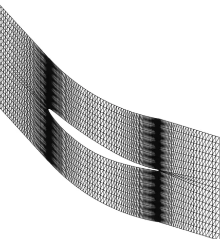
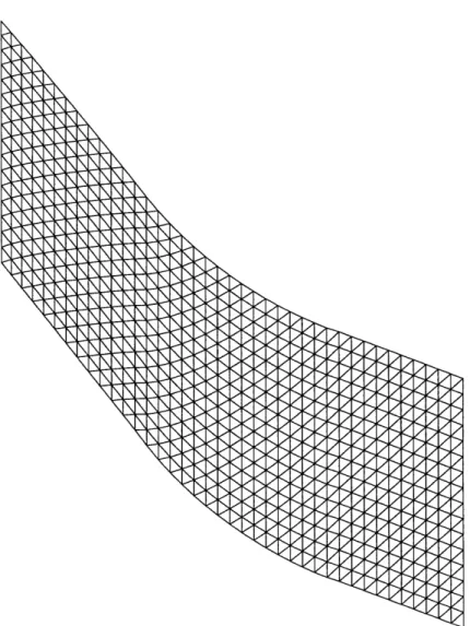
As can be seen on figure 2-2, high levels of grid resolution are needed along the blade in order to describe the actual blade shape. The modeling concept which is developed here is to completely remove the blade, in order to further coarsen the

(37)

Figure 2-3: Computation mesh for a stator blade row with blade modeling

mesh as shown on figure 2-3.

The modeling methodology used for this third step is similar to the one used for the first two: the chosen model will seek to duplicate the important effects that the blade has on the flow using large scale features.

(38)

2.4.1 Model Elements

Models for turbulence and viscous effects have been developed in the previous para-graphs by considering the effects of the phenomena on the flow and duplicating these effects using large-scale features.

A similar approach can be used for blade modeling. As the two main effects of a blade row on a flow are to apply forces - whether they are viscous or pressure forces - _{and blockage, it can be argued that a blade row can be removed from a} flow computation if the equivalent forces and blockage are still applied through the use of a physically sound model. The blade model developed in this research will be constituted of distributed body forces and distributed heat sources. A blockage factor should also be included, but this will not be done here for simplicity. The cost of this simplification will appear in the following paragraphs. A blockage factor is expected to be included in future refinements of the model though.

In contrast to Denton's viscosity model, which only made use of body forces aligned with the flow to create loss, the model developed here will feature body forces both aligned with and orthogonal to the flow, to provide loss as well as turning and diffu-sion.

As stated above, the blade model will also feature distributed heat sources. Whereas the presence of body forces in the model is consistent with the idea of replacing a blade by equivalent forces, the distributed heat sources are not a representation of flow physics, and their relevance will appear later as an important tool in controlling the flow thermodynamics.

2.4.2 Model Requirements

The blade model developed here is expected to be used to replace blade rows in a multistage compressor computation. It is therefore necessary for this model to:

(39)

* duplicate the effect of the blade row on the typical unsteady flow encountered in multistage compressors, in particular the physical phenomena known to affect compressor performance.

* provide consistent boundary conditions for the blade rows placed directly up-stream and downup-stream in the compressor.

Both these requirements will be examined below.

Unsteady Flow Behavior

The unsteady flow in a compressor blade row consists of a succession of patches of irro-tational flow and vortical flow. The vortical flow is shed by the blade row immediately upstream, and consists of a wake, a tip leakage vortex, and a number of additional vortices. The blade model will be expected to duplicate both the irrotational and vortical flow behaviors.

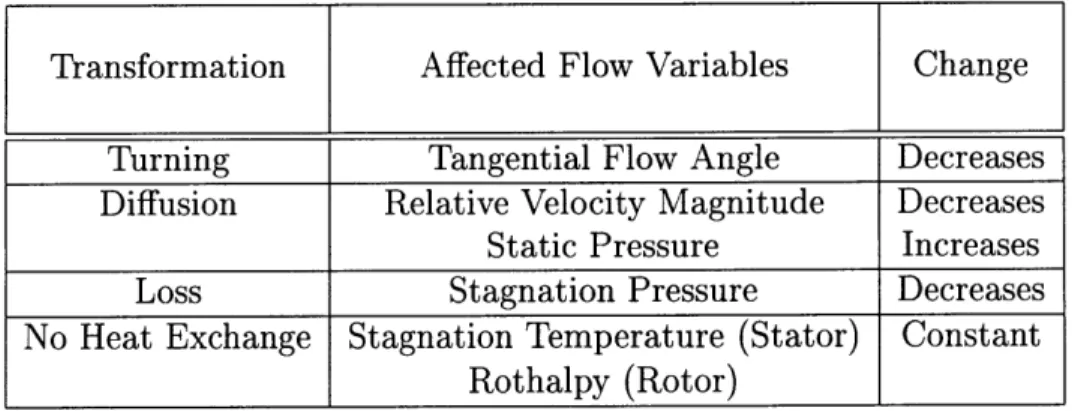
Irrotational Flow Behavior Table 2.1 summarizes the different transformations undergone by irrotational flow as it proceeds through a compressor blade row. For each transformation, table 2.1 also indicates the flow variables which are affected.

Transformation Affected Flow Variables Change

Turning Tangential Flow Angle Decreases

Diffusion Relative Velocity Magnitude Decreases

Static Pressure Increases

Loss Stagnation Pressure Decreases

No Heat Exchange Stagnation Temperature (Stator) Constant Rothalpy (Rotor)

Table 2.1: Irrotational Flow Behavior in Stator Blade Row

(40)

listed in the second column of table 2.1 are matched when a blade row is replaced by its model. The radial flow angle will be added to the list for completeness.

If the above flow variables are matched by the model, other variables will be matched as well:

* The three components of the velocity will be matched because velocity magni-tude and the two flow angles are matched

* Static temperature will be matched because stagnation temperature and veloc-ity magnitude are matched

* Density will be matched because static pressure and temperature are matched

* Entropy will be matched because stagnation pressure and stagnation tempera-ture are matched

In conclusion, the model will match all aerodynamic and thermodynamic flow variables.

Vortical Flow Behavior A review of vortical flow physics in multistage turboma-chines is provided by Taylor [27]. In addition to the transformations listed above for the irrotational flow, the vortical flow undergoes additional transformations, each of which leads to additional model requirements:

Viscous Dissipation Wakes and vortices are viscously dissipated as they pro-ceed through the compressor. When a blade row is replaced by a body force and heat source model, it might be deemed important that the dissipation still continues to take place in a similar fashion in the modeled region. The use of the blade row model with a Navier-Stokes solver will therefore be considered in chapter 6.

(41)

Wake and Tip Vortex Stretching The wake shed by a blade row is chopped into vortical fluid filaments by the downstream blades. These filaments are then stretched as they proceed through the blade row because of two phenomena: the increase in cross-flow area, and a rotation of the filament due to the velocity difference between the blade pressure and suction sides. Similar phenomena affect tip vortices. Stretching of wakes and tip vortices lead to a reversible recovery of the excess kinetic energy present in these vortical structures into static pressure.

In order to capture wake and tip vortex stretching, the model must duplicate both cross-flow area change and filament rotation. The former is linked to flow turning, and is already part of the model requirements associated with the irrotational flow behavior. The latter requires in addition that the model should not be axisymmetric.

Interaction with Blade Boundary Layer Recent work by Valkov [28] has shown that wakes and tip vortices do interact with the boundary layer of the down-stream blade, and that this interaction affects the compressor performance.

This interaction phenomenon cannot be easily captured by the blade row model, because of the absence of blades and therefore of boundary layers. The time-averaged impact of wake and tip-vortex boundary layer interaction can still be accounted for by the model though, by making the model elements variable with the local flow conditions. This allows the model to process irrotational and vortical fluid in different fashions, and to reflect the effect of vortical fluid-boundary layer interaction on an averaged basis.

Table 2.2 summarizes the specific transformations undergone by the vortical flow as it proceeds through a compressor blade row, and the additional model requirements which follow.

(42)

Transformation Model Requirement

Stretching Non-axisymmetric model

Dissipation Use of a Navier-Stokes solver

Interaction with boundary layer Model elements variable with local flow condition

Table 2.2: Rotational Flow Behavior in Stator Blade Row and Subsequent Model Re-quirements

Boundary Conditions

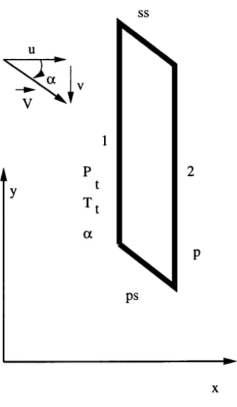
In subsonic flow, as is the case for all flows considered in this research, four of the five boundary conditions needed to solve the Navier-Stokes equations are imposed at the upstream boundary, and the fifth one at the downstream boundary [17]. The upstream boundary conditions are the stagnation pressure, stagnation temperature and the two flow angles, while the downstream boundary condition is the hub static pressure.

Let then a stator blade row model be considered in between two discrete rotor blade rows (Figure 2-4)

The static pressure on plane 2 therefore acts as the downstream boundary condi-tions for the upstream rotor. The stagnation pressure, stagnation temperature and the two flow angles on plane 3 acts as the upstream boundary conditions for the downstream rotor.

To meet its requirement to provide consistent boundary conditions to the blade rows directly upstream and downstream, the model needs to accurately provide the static pressure at its upstream boundary, and the stagnation pressure and temperature and flow angles at its downstream boundary.

Backpressure fluctuations In modern compressor designs, the spacing be-tween neighboring blade rows is small, typically 20 to 40 percent of the stator axial

(43)

Boundary Conditions Boundary Condition

Ptot ,Ttot , 1 P

1

Upstream Rotor 2 Stator Model 3 Downstream Rotor 4

Figure 2-4: Stator model embedded between two rotors

chord. The high static pressure region which develops around a blade leading edge is therefore felt at the trailing edge of the blade directly upstream. Recent work by Graf [15] has shown that the backpressure fluctuation felt by a rotor as it moves relative to a downstream stator affects the rotor flow and the time-averaged rotor performance. This phenomenon needs to be captured by the blade row model developed here, and the static pressure field at the inflow boundary of the model region should therefore be non axisymmetric. This results in the requirement that the model should be non axisymmetric too, a requirement which has already been stated in order for the model to capture wake and tip vortex filament rotation.

2.4.3 Blade Modeling: Summary

A blade model consisting of distributed body forces and heat sources will be developed in this thesis. This model will first be constructed in steady flow, before tackling the more challenging unsteady flow case.

(44)

Steady Flow Model In steady flow, only the irrotational flow requirements apply. The model will be required to match all aerodynamic and thermodynamic flow vari-ables. Because the flow is uniform, no viscous dissipation takes place, and the model can be used with an Euler solver.

This option will be preferred, because it makes the computation of the model elements more straightforward, as will be seen in chapter 3.

Unsteady Flow In unsteady flow, the model can be used with a Navier-Stokes solver in order to feature flow nonuniformities dissipation. In addition, in order to capture all the unsteady flow phenomena known to affect compressor performance, the model should be non axisymmetric, and model elements should respond to local flow conditions. For the sake of simplicity, none of these two features will be included in the model developed here, nor will the model include a blockage factor, and the cost of this simplification on the effectiveness of the model will be assessed.

(45)

CHAPTER

3 DEVELOPMENT OF A BLADE ROW

MODEL IN STEADY FLOW

Chapter 2 introduced the concept of modeling in computational fluid dynamics and described the elements used to construct a blade row model, namely distributed body forces and heat sources. This chapter will describe how a model is constructed for a given blade row in steady flow at a given operating point. An analytical approach will then be developed in chapter 4 to show the effectiveness of the model for two-dimensional flows, and test cases will be presented in chapter 5 for three-two-dimensional flows. This development of the steady flow model will be followed by proposed guide-lines for further improvement.

3.1 Prerequisites to the Construction of a Model

As described in Chapter 2, a blade row model is a large-scale representation of small-scale effects that the blade row has on the flow. In order to construct a blade row model, it is necessary to know these effects to a certain extent. The detail to which these effects need to be known depends on the precision required from the model.

One extreme is to know the flow variables exclusively at the inflow and outflow of the blade row to be modeled, but not in between. The model developed is then

(46)

referred to as an actuator disc. Its role is to transform given inflow conditions into given outflow conditions, but the way flow variables evolve in between is not pre-scribed. At the other end of the scale, the flow is known throughout the flow domain, and a model can be developed to duplicate not only the inlet/outlet behavior of the blade row, but also the way flow variables change through it.

The latter approach is chosen for this research, and it will be assumed that, prior to the developments below, the flow in the blade row to be modeled has been computed at the chosen operating point.

3.2 Compatibility of the Model with the NEWT

Code

The equations of fluid dynamics are just equations of a particular form of continuum mechanics. Hence, the computation of fluid flows is similar to that of other continuum mechanics problems such as elasticity problems, in the sense that the continuum equations are transformed into algebraic equations by discretizing the computational domain into a finite number of elements. These algebraic equations can then be solved using various numerical methods.

There are two very different ways to discretize and solve the equations of fluid mechanics:

* Finite Difference equations result from the discretization of the differential form of fluid mechanics equations. The computational domain is discretized into

discrete points.

* Finite Volume equations result from the discretization of the integral form of fluid mechanics equations. The computational domain is discretized into finite

(47)

More details on the differential and integral forms of the equations of fluid me-chanics and on the discretization procedures alluded to above can be found in [17].

All the flow computations performed in this research make use of the NEWT CFD code developed by W.N. Dawes [10]. This is not a model requirement though: the model has been designed to be as portable as possible. A concise description of NEWT is provided in appendix A.

NEWT is a finite-volume code, and for full compatibility with the model, body forces and heat sources are also computed in finite volumes rather than at discrete points. For identical reasons, the model makes use of the integral form of the equations of fluid mechanics rather than of their local differential form.

3.3 Computation of the Model Elements

In this section, the equations of fluid mechanics and thermodynamics are used to show how a body force and heat source model can be constructed for a blade row at a given operating point, provided the flow in this blade row has been previously computed. For reasons which will appear below, aerodynamics and thermodynamics are considered separately.

As explained above, the model is developed using the integral form of the equa-tions, and is based on a control volume approach.

3.3.1 Flow Aerodynamics

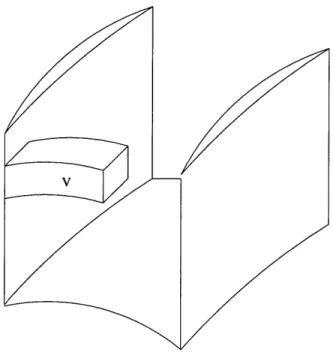
Let then a control volume be considered in the blade passage (figure 3-1). The control volume will be referred to as V, and the surface surrounding it as A. No precise description will be given at this point of the actual shape of the control volume or its location in the blade passage, apart from the fact that, in the most general case, some part of the surface A will be in contact with a solid surface, either the blade

(48)

row or an endwall. A will therefore consist of A1, which is in contact with a solid

surface, and A2, which is not.

Figure 3-1: Typical Control Volume in a Blade Row

The integral form of the continuity and momentum equations of fluid mechanics will be written for this control volume in two cases:

* Case 1: The blades are physically present, the flow is viscous and the walls are

adiabatic. This flow will be referred to as the real flow.

* Case 2: The blades are removed and replaced by their model. The flow is

nonviscous and there are distributed body forces and heat sources. This flow

will be referred to as the model flow.

The two sets of equations will be compared, and the values of the body forces and heat sources will be found from this comparison.

The integral continuity and momentum equations of fluid mechanics are, in their most general form [2]:

(49)

=- p - "- dA A

fpVdv +

i

V A

pV(V

- fJ pndA + A A

II

P7

dV

v (3.2)

All flows considered in this chapter are steady, so all time derivative terms will be set to zero.

Some of the integrals in these equations will also vanish depending on which one of the two cases is considered.

Case 1

In this case,

* V

vanishes on all solid surfaces. All integrals where the velocity multiplies an integrand will only be evaluated on surface A2, the fraction of the control

volume boundary surface which is not in contact with a solid.

* If the effects of gravity are neglected as is commonly done for low-density fluids, body forces will vanish from all equations.

With these simplifications, the general integral equations become:

fpV

-

dA = 0

(3.3)

A₂

Af

PV(

A2 T)dA = -A pndA + f A ff pdV V (3.1) - ndA (3.4)

(50)

Case 2

In this case, the only possible simplification comes from the fact that the flow is nonviscous. All integrals where the viscous stress tensor multiplies an integrand will therefore vanish. With this simplification, and separating integrals on surfaces A₁ and A2 where needed for clarification, the general integral equations become:

5V • + j V *dA dA 0 (3.5)

A1 A2

J

V (V(V -. )dA +

J

V ( V - n )dA = -

J

n dA +

fT

dV

A1 A2 A V (3.6)

In these equations and in all equations which will follow, the tilde(~) symbol is used to denote the model flow variables from the real flow ones.

The following sections will analyze how to compare these two sets of equations in order to extract the model from them.

Identity of Two Flows

To claim that a flow model has been adequately developed to simulate an actual blade row, the flow must be duplicated when the blade row is replaced by its model, i.e. flows in cases 1 and 2 must be identical.

The notion of identity of two flows needs to be defined. Due to the finite volume structure of the computation code, the computation domain is discretized using three types of structures: nodes, faces and volumes. Based on this discretization, two approaches can be taken in comparing two flows:

* The strong approach: compare the flow variables at each node

A computational model for multistage axial compressor design

A

©

A,/

[~-

mA

')9ig~

A

ACKNOWLEDGMENTS

CONTENTS

LIST OF FIGURES

LIST OF TABLES

NOMENCLATURE

Roman

Q

Greek

Subscripts

flowblade

II

Superscripts

Other useful notations

CHAPTER

1

INTRODUCTION

1.1

Evolution in Compressor Design Methods

1.2

Motivation of the Research

1.3

Statement of the Problem

1.4

Contributions of the Thesis

1.4.1

Modeling in Turbomachinery Fluid Dynamics

1.4.2

Expected Contribution to On-Going and Future

Re-search Efforts

1.5

Organization of the Thesis

CHAPTER

2

MODELING IN TURBOMACHINERY

COMPUTATIONAL FLUID DYNAMICS:

KEY CONCEPTS

2.1

Parametric Dependence of Computation Power

on Problem Length Scales

2.2

First Step: Turbulence Modeling

2.3

Second Step: Viscous Effects Modeling

2.4

Third Step: Blade Modeling

2.4.1

Model Elements

2.4.2

Model Requirements

1

2.4.3

Blade Modeling: Summary

CHAPTER

3

DEVELOPMENT OF A BLADE ROW

MODEL IN STEADY FLOW

3.1

Prerequisites to the Construction of a Model

3.2

Compatibility of the Model with the NEWT

Code

3.3

Computation of the Model Elements

3.3.1

Flow Aerodynamics

fpVdv +

i

pV(V

II

dV

* V

fpV