Design and development of an improved two-axis meso-scale electro-magnetic actuator for a flexure based nano-positioner

Design and Development of an Improved Two-Axis Meso-Scale Electro-Magnetic

Actuator for a Flexure Based Nano-Positioner

by

Prosper M. Nyovanie

Submitted to the Department of Mechanical Engineering

June 2013 in Partial Fulfillment of the

Requirements for the Degree Bachelors of Science in

Mechanical Engineering

@ 2013 Massachusetts Institute of Technology

All rights reserved.

ARCH1$

f

OF TECHNLOGY

<JUL31 013

Signature of Author...---..---

-

---.---.

r

---Departmtof MVfchpnical Engineering

May 2013

Certified by

...

Martin L. Culpepper

Associa

rofessor of Mechanical Engineering

Thesis Supervisor

Accepted by

...-...---

---Annette Hosoi

Professor of Mechanical Engineering

Undergraduate Officer

Design and Development of an Improved Two-Axis Meso-Scale Electro-Magnetic Actuator for a Flexure Based Nano-Positioner

by

Prosper M. Nyovanie

Submitted to the Department of Mechanical Engineering June 2013 in Partial Fulfillment of the

Requirements for the Degree Bachelors of Science in Mechanical Engineering

ABSTRACT

The intent of this thesis is to provide theory behind the design and development of an improved two-axis meso-scale electro-magnetic actuator for a low cost metal flexure nano-positioner. Three such 2-axis actuators can be combined to give the nano-positioner 6-degrees of freedom. The developed system will remove the cost barrier to technologies that require high precision actuation, like optics alignment and data storage. This work involves use of a new combination of the following technologies 1) Electro-magnetic Lorentz coil actuation (moving magnet), 2) flexural bearings and 3) rapid printed circuit board (PCB) heat dissipation. Simulations using Solidworks and Matlab were employed to determine how the actuator system behaved. It was determined that the actuator was required to provide 0.17N and 0.12N in plane and out of plane forces, respectively, to provide the target ± 20gm range of motion. The actuator dissipates 11W of heat when achieving maximum range, which raises the temperature of the Lorentz coils from room temperature to 369K, a temperature below the maximum permitted temperature of 413K. The analysis has shown that it is feasible to design and make a two-axis electro-magnetic actuator that can be incorporated into a six-axis flexure based nano-positioner.

Thesis Supervisor: Martin L. Culpepper

AcKNOWLEDGEMENTS

This work was only made possible through the great support that I received during the duration of this project. First of all I would like to thank Robert Panas, who introduced me to the PCSL lab three years ago as his UROP. He has served as a great mentor and advisor to me not only for this project but also for navigating my way through the opportunities available at MIT.

I also would like to thank Lucy Du for all the help she gave me with the

simulations and for listening to and offering feedback on some ideas that I had during the project.

I would also like to thank Professor Martin Culpepper for the mentorship and guidance over the past three years that he has been my UROP PI. His advice has been invaluable for both this project and in defining my goals for after MIT.

Lastly I would like to thank the Mechanical Department for the great instruction, support and opportunities that they have provided during the past four years that I have

CONTENTS

Contents

3

Acknowledgem ents

...

5

Contents

...

6

Figures

... 8

Tables

... 8

Chapter 1

...

10

M otivation

...

10

Figure 1. 1: HEXFLEX flexure bearing

...

11

1. 1 Prior art and actuator selection

...

11

1.2.1 Piezoelectric Actuators

...

12

1.2.2 Electrotherm al Actuators

...

12

1.2.3 Electrostatic actuators

...

12

1.2.4 Electrom agnetic actuators

...

13

1.2.5 A ctuator Sum m ary

...

14

Chapter 2

...

16

2.1 Electrom agnetic actuators

...

16

2.2 Lorentz coil forces

...

16

Chapter 3

...

19

3.1 Flexure bearing

...

19

3. 1.1 Flexure bearing properties

...

20

3.1.2 Flexure theory

...

21

3.2 HEXFLEX

...

22

3.3 Final HEXFLEX design

...

23

Chapter 4

...

25

4.1 Printed circuit board design

...

25

4.2 Therm al dissipation m odes

...

25

4.2.1 Conduction

...

26

4.2.2 Convection

...

28

4.3Therm al resistance m odel ... 29

4.4 Therm al Design for printed circuit boards... 30

4.4.1 Printed circuit lam inate... 32

4.4.2 Copper Pour ... 32

4.4.3 Therm al Vias... 32

Chapter 5... 34

5.1 Flexure/HEXFLEX Sim ulation ... 34

5.2 EM sim ulation... 37

5.2.2 Sim ulation results and analysis ... 38

5.2.3 Sum m ary of results ... 42

5.3 Therm al sim ulation... 43

5.4 Sum m ary of results ... 46

Chapter 6... 48

7.1 Sum m ary of design and developm ent... 48

FIGURES

Figure 2.1: a) Cross section view of a three pole alternating magnet configuration with actuator coils suspended above the magnets. b) Individual plan views of the stacked

coil actuator architecture... ... 17

Figure 2.2: Close up view of the 3 pole magnetic actuator architecture. [5]... 18

Figure 3.1: shows a cantilevered beam deforming under a load P [10]... 21

Figure 3.2: Spring model for actuator and flexure bearings ... 22

Figure3.3: HEXFLEX developed by Culpepper et al. showing example displacements for give tab displacements. (x) shows direction into plane, (.) shows directions out of plane, hollow arrows show actuator inputs and shaded arrows show stage displacem ents... .. 23

Figure 3.4: Redesigned HEXFLEX showing its key features ... 24

Figure 4.1: Heat transfer via the copper walls of a thermal via... 33

Figure 5.1: a) General meshing used for the simulation. b) local mesh control applied to flexures to improve simulation accuracy ... 35

Figure 5.2: In plane actuation of HEXFLEX with 0.17N applied to two of the paddles. Arrows show the direction in which the forces are applied... 36

Figure 5.3: Out of plane actuation of HEXFLEX with 0.12N applied to normal to all three paddles. ... .... --...-... 36

Figure 5.4: Results for X-Actuator simulation Ftotalx vs. bcoil including variation in parasitic force error as a percentage of Ftotalx. This graph is similar to the one for Ftotalz vs. bcoil... .... .... 39

Figure 5.5: Results for Z-Actuator simulation Ftotalz vs. tcoilCuweight including variation in parasitic force error as a percentage of Ftotalz. This graph is similar to the one for Ftotalx vs. tcoilCuweight... 40

Figure 5.6: Results for Z-Actuator simulation Ftotalz vs. Current including variation in parasitic force error as a percentage of Ftotalz. This graph is similar to the one for Ftotalx vs. C urrent. ... .... 41

Figure 5.7 :Results for Z-Actuator simulation Ftotalz vs. height of coils above magnet surface above including variation in parasitic force error as a percentage of Ftotal_z with Current=8A. This graph is similar to the one for Ftotalx vs. Height... 42

Figure 5.8: Holes used to allow the introduction of copper posts into the PCB... 44

Figure 5.9: Thermal chart for results of one of the simulations... 44

Figure 5.10: The highest temperature occurs along the sides that do not have copper posts and these points along the same plane as the coils. ... 45

Figure 5.11: Final maximum temperature for 1.575mm PCB board vs. the number of copper posts in the PCB ... 46

TABLES

Table 1.1 Qualitative comparisons of electromagnetic actuator species ... 14

Table 1.2 Typical small scale Nano-positioner actuator performance [6]... 15

Table 5.1: Results from flexure simulation... 36

Table 5.2: Parameters for Lorentz coils simulation... 38

Table 5.3: Standard simulation values ... 38

Table 5.4 Summary of simulation results ... 42

CHAPTER

1

INTRODUCTION

Motivation

The intent of this thesis is to provide theory behind the design and development an improved 2-axis electro-magnetic actuator for a low cost metal flexure

nano-positioner. The 2-axis actuators if properly designed can then be employed to produce 6-axis motion of a HEXFLEX stage [1]. This work involved use of a new combination of the following technologies 1) Electro-magnetic Lorentz coil actuation (moving magnet) 2) flexural bearings 3) rapid printed circuit board (PCB) heat dissipation. These

technologies will be combined to produce an inexpensive way of providing nano-meter accurate motions over a range of about 20pm x 20gm x 20m and at a bandwidth of

100Hz while maintaining nano-meter range repeatability. The flexure design will involve special consideration to make it compatible with the attachment of silicon based strain gauges that being developed by Panas [2]. The gauges will provide better control of the actuation because of the feedback capabilities that will allow closed loop control.

The results of this thesis could prove useful to removing the barriers to some technologies that require high precision actuation or manipulation but are hindered by the high costs of current nano-positioners. Some of the technologies include fiber optic

aligners, manufacture of small components, data storage and biomedical research. The addition of compatibility with silicon strain gauges that have a high gauge factor will allow for even better actuation control at a much lower price [2].

The reduction in the cost of the nano-positioner, actuator and sensor combination, will provide a better performance to cost ratio for nano-positioners. This development

could lead to removal of one barrier hindering the economic feasibility of

nano-positioners for new applications in research and in industry.

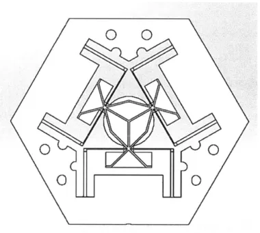
One of the biggest issues that this thesis work will tackle is the range limitation of

current actuators. The range of the actuator is dependent on the design of the HEXFLEX

shown in figure 1.1, and the force the actuators can provide. This thesis project will

mainly focus on the actuator part and so most of the design work will entail finding ways

to increase the force generated by the actuator. The maximum force is dependent the

amount of current that can be safely passed through the coils, without overheating and the

design of the coils.

/

Figure 1.1: HEXFLEX flexure bearing

1.1 Prior art and actuator selection

A number of different meso- scale actuator designs have been developed to

achieve nano-level accuracy and precision. The designs can be divided into four main

categories 1) Piezoelectric, 2) Electrothermal, 3) Electrostatic and 4) Electromagnetic.

These different actuators have their own unique pros and cons.

0 0

NJ

0

1.2.1 Piezoelectric Actuators

Piezoelectric actuators are made from materials that undergo dimensional changes when a voltage is applied across them. The change in dimension is typically directly proportional to the electric field applied across the material[3].Piezoelectric actuator are have high levels of resolution and can achieve sub-nanometer level resolution. The actuators produce high levels force and emit a couple of mill-watts of power [4]. This means that the actuators have a high level of efficiency. Piezoelectric actuators have a

fast response but can only operate over a limited distance. The fabrication process and integration of piezoelectric actuators into an actuation system is complex [5] [6]. Also errors are introduced into the system because hysteresis and steady state drift making it necessary for feedback loop to be used.

1.2.2 Electrothermal Actuators

Electrothermal actuators take advantage of thermal expansion in materials as a means to provide actuation. Electrothermal actuator can produce high forces but like piezoelectric actuators, they can only produce small displacements. Electrothermal

actuators have been successfully used to drive six-axis nano-positioners [5]. The fabrication process is complex as electrothermal actuators are normally made using a

silicon micro-fabrication process [6]. Response time of these actuators is limited by how fast the material can be heated or cooled. Electrothermal actuators are unsuitable for manipulating temperature sensitive materials since they operate at high temperatures of around 6000C [5]. The heat operating temperatures can also cause thermal gradients and hence lead to thermal error in both the bearings and sensors.

1.2.3 Electrostatic actuators

Electrostatic actuators rely on the principle of electrostatic attraction. Electric charge is deposited on two surfaces that are in close proximity to each other, the resulting

electric force is what is used for actuating the system. These actuators have a simple fabrication process but are will be difficult to integrate into nano-positioner systems. Electrostatic actuators tend to have lower forces compared to the other actuator types. The major problems with this type of actuator are gap field breakdown, gap

contamination and the need to use high voltages in the order of lOs-lOOs of volts [5]. Electrostatic actuators also suffer from limited in- and out-of-plane range making it difficult apply them to more than 2 degree-of-freedom applications. There exist example of systems that have used electrostatic actuator for 6-axis actuation but their range of motion was limited [5].

1.2.4 Electromagnetic actuators

Electromagnetic actuators rely on the interaction of electric and magnetic fields to produce forces. Electromagnetic actuators can provide large forces over a large range of motion [6]. These actuators can be designed in such a way that they can provide a force with high degree of linearity with current that the need to use sensors for some

applications can be eliminated [5]. Electromagnetic actuators have lower command voltages compared to electrostatic actuator making them easier to implement. There are three main types of electromagnetic actuators that were are going to consider; 1) variable reluctance, 2) moving magnet and 3) moving coil.

1.2.4.1 Variable Reluctance Actuator

Variable reluctance actuators work of the reluctance principle in magnetic circuits. They are capable of producing high forces and have high resolution. The main limitation with variable reluctance actuators is that can only operate in one axis.

1.2.4.2 Moving-Magnet Actuator

Moving magnet actuators, unlike variable reluctance actuators, can provide both single and multi-axis actuation. Moving magnet and moving coil actuators are similar but differ in where the permanent magnets and coils are placed. In moving magnet actuators, magnets are attached to the flexure bearings, allowing them to move with bearings, and the coils are in a fixed position, hence the name moving magnet actuator. Having the coils in a fixed position makes it easier to transfer dissipated heat from the coils allowing more current to safely flow through the coils without overheating. At the same time addition of magnets/mass to the flexure causes the system to have a low resonance frequency [5].

1.2.4.3 Moving-Coil Actuator

Moving coil actuator is similar to the moving magnet actuator described in section 1.2.4.2 above. The main difference is now the coils are the ones that are attached to the flexure and the magnets are attached to a fixed position. This is easier to fabricate compared to moving -magnet actuator [6]. Cooling the coils in moving-coil actuators is more difficult leading to a lower safe current limit for moving-coil actuators compared to moving-magnet actuator. Because of the lower current limit, the force generated by moving-coil actuators is lower than the force generated by moving- magnet actuators. Power dissipation from the moving coils goes through the flexure bearings causing thermal errors in both the sensors and flexure repeatability.

1.2.5 Actuator Summary

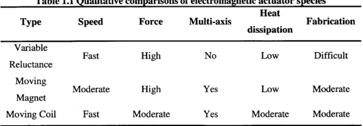
The three most often used electromagnetic micro-actuators are 1) variable reluctance, 2) moving magnet and 3) moving coil. Table 1.1 below shows the qualitative comparison of the three actuators [5].

Table 1.1 Qualitative comparisons of electromagnetic actuator species

Heat

Type

Speed

Force

Multi-axis

dissipation

Fabrication

Variable

Fast High No Low Difficult

Reluctance

Moving Moderate _{High Yes Low}

Moderate Magnet

Moving Coil Fast Moderate Yes Moderate Moderate

Variable reluctance actuators have great response, high force output and low thermal heat dissipation. These qualities would have made variable reluctance actuator an idea for 6-axis nano-positioners but the fact the fact that they only have one 6-axis actuation rules them out of further consideration for use in six-axis nano-positioner. Moving coil and

moving magnet actuators can both be used for six-axis nano-positioner actuation and so will be compared with other types of actuators.

As seen from table 1.1 above variable reluctance actuators are not suitable for multi-axis actuation. The summary of the performance of the remaining actuators, Electrostatic (ES), Moving coil, Moving magnet, Piezoelectric (PE) and Electrothermal (ET), are summarized in the table 1.2 below [6]

Table 1.2 Typical small scale Nano-positioner actuator performance [6] Ease of

Stoke Bandwidth Force Footprint Heat Ease of

Type

MDOF

(Pm) (kHz) (mN) (pm2_{) Dissipation fabrication}

integration*

ES 100 10 0.001 104 Low Good Difficult

Moving 10 1 0.1 106 Moderate Difficult _Good

coil

Moving 100 0.1 10 106 Low Good _Good

magnet

PE 1 100 0.1 102 Low Difficult Difficult

ET 100 1 10 102 High Good Good

*Note: MODF integration is a qualitative measure of how easily the actuator can be integrated in a Multi-Degrees of Freedom system.

Piezoelectric actuator and moving coil actuator have ranges that are less than the required ±20pm range of motion and so can be crossed out even though they might have good qualities like high force and MODF integration respectively. Electrothermal actuators have high operating temperatures that make unsuitable for manipulation of temperature sensitive material like biological cells. This leaves electrostatic actuators and moving magnet actuators as the remaining options. Moving magnet actuator has a better ease of MDOF integration whereas electrostatic have a limited range when applied to multi-actuation. Moving magnet is the best option of the actuators that considered in this section. Section 2 will look into the theory governing how they work.

CHAPTER

2

THEORY- ELECTROMAGNETIC ACTUATOR

2.1 Electromagnetic actuators

Electromagnetic actuators, as described in section 1.2.4, generate forces through interaction between electric and magnetic fields. They are capable of generating high forces and can be designed to have a high current to force linearity. Three main types of electromagnetic actuators were considered namely variable reluctance, moving magnet and moving coil actuators. It was shown in section 1.2.5 that moving magnet actuator is the most suitable actuator for this project because of its

" High force output

" Compatibility with multi axis actuation * Low heat dissipation

* Ease of fabrication

Moving magnet actuator generates it forces as a result of Lorentz coil forces.

2.2 Lorentz coil forces

A force is generated on a charged particle when it moves relative to a permanent magnetic field. Lorentz coil forces employ the same principle to produce forces whereas this case the moving charged particles are electrons moving through a conductor. The windings are fixed and so cannot move relative to each other, this means that the magnetic fields that are caused by current going through the winds do not contribute to the Lorentz forces [5]. Therefore the Lorentz forces will only depend on magnetic fields

caused by permanent magnets. The total Lorentz forces are calculated by integrating the following equation:

Fcol = fo il(r) x B(r)dl 2.1 Also total moment about a reference point 0 is

Mcoilo = f (r - ro) x il(r) x B(r)dl 2.2 where i is the current flowing through the windings, r is the position vector of the current, I is the current direction, B is the local magnetic field at the current increment, dl is the length increment, r, is the position vector of the reference point, and L is the length of the coil.

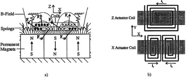
The actuator has a three pole alternating magnet configuration that is described by Golda [5] shown the figure 2.1 a below. The actuator consists of three permanent magnets and two sets of actuator coils. The design of the coils is shown in figure 2. 1b below. .

B-Field-ZActuatorCoil

N F g

I

Figure 2.1: a) Cross section view of a three pole alternating magnet configuration with actuator coils suspended above the magnets. b) Individual plan views of the stacked coil actuator architecture.

The coils are stacked on top of each other separated by an electrical insulator. The coils are capable of generating forces along different axes independent of each other allowing for two axes actuation. Actuator forces are primarily generated by the segments that are

parallel to the y- direction. Coil segments that are parallel to the x- direction generate negligible forces because they are in regions that have negligible magnet fields.

The interaction of magnetic fields of the individual magnets produces a magnetic an overall magnetic field that is different from that of an individual magnet. Fourier transform was used to simulate and model the 3-dimensional magnetic field generated by the magnetic array. Figure 2.2 below shows a close up view of the 3 pole alternating magnetic array.

cY(x,y,c/2).,

x

z

M

MC

Mt

Figure 2.2: Close up view of the 3 pole magnetic actuator architecture. [5]

The 3 pole alternating magnetic architecture has an even surface charge distribution function of a(x,y,1 c) that consists of three top-hat functions [5]. The double Fourier transform of this distribution is [5]

0(k. , k,) = Sin! - bky(sinak. - sin 2ak.,) 2.3

kxk 22 2

where a, b, c are dimensions of the magnets, M is the uniform magnetization along the z-direction of the magnet, ky and k, are separation constants. Equation 2.3 is going to be used in developing the simulation to predict the forces that are generated by the actuator.

CHAPTER

3

HEXFLEX

DESIGN AND THEORY

3.1 Flexure bearing

Bearing design is extremely important not only to designing a high precision manipulation system like a nano-positioner, but to all mechanical systems that have moving components. Bearings allow components in a system to move relative to each other. Without bearings movement of components relative to each other would be hindered and some mechanical systems would either stop working or fail regularly. Some of the main considerations when con sidering a bearing design for a system include:

" Range of motion: What are the limits on how system can move?

* Speed and acceleration limits: How fast components will move relative to each other?

* Applied loads: What are the safe loads for the system? * Repeatability: Is motion reproducible?

* Accuracy: Does the bearing allow or hinder desired motion or positioning? * Resolution: Are small increments in motion possible?

* Friction- causes wearing and dissipates heat

* Thermal performance: How does temperature variation affect the system? * Cost?

3.1.1 Flexure bearing properties

Flexure bearings have distinct advantages over sliding, rolling, and fluid bearings. Surface finish limits the performance of sliding and rolling bearing; since it's impossible to have a perfect surface these bearing tend to be not suitable for high precision

applications. Fluid bearings are prone to dynamic and thermal effects and so they also are not suitable for some high precision applications. Flexure bearings work based of

stretching of billions of atomic bonds. The large number of bonds involved in the relative motion, average out the motion producing a smooth motion with sub-angstrom resolution [4]. Here are some of the important properties of flexure bearings:

* Speed and acceleration: Is limited the natural frequency of the system and stress levels in the flexures.

* Range of motion: Is generally small because flexures operate in the elastic regime of the material to prevent permanent deformation of the flexures. Monolithic flexures bearings have a range of motion to bearing size ratio on the order of

1/100[4]. The limit in range is normally not a problem for systems that require very high precision over short ranges, and will not be a problem for the nano-positioner design.

* Applied load: Flexure bearings can be designed support huge loads. That being said the expected load has to be taken into consideration when designing the flexure.

* Accuracy: This is dependent on the machining process for making the flexure. Perfect motion for monolithic flexures is unattainable because of inaccuracies in machining, bending of structure and external applied loads.

* Repeatability: Monolithic flexures are highly repeatable down to sub-angstrom range [4]. Repeatability influenced by stress level and bending hysteresis which

could lead to permanent deformation of in the flexure.

* Resolution: As mentioned before flexures have very fine because of the averaging out of motion that occurs at the atomic scale within the material. Therefore system resolution is limited by the resolution of the actuators.

* Require life: Is infinite as long the flexure is properly designed to prevent excessive strains and stresses.

* _{Cost and manufacturability: Flexures are easy to manufacture and are generally} inexpensive.

3.1.2 Flexure theory

In the simplest form flexure bearings are deforming beams. Because the flexure bearings' similarity to beams, beam-bending equation can be applied to them to analyze how they are going to behave. The figure 3.1 below shows a cantilevered beam bending under a load

lamp _L

Unloaded Beam

_h

_I

t

Loaded Beam

Figure 3.1: shows a cantilevered beam deforming under a load P [10]

The deflection of the tip of the beam is defined by the following equation

P L3

6 = --

_3.1

3EI

where 8 is the tip deflection, P is the load applied to the beam, L is the length of the

beam, E is the Young's modulus of the material and I is the moment area of inertia. L and

I depend on the geometry of the beam and E is a material property. Therefore the

behavior of the bearing is dependent on material properties and the geometry of the

flexure and not on surface finish that is hard to control. The behavior of flexure bearings

is also dependent on the boundary conditions of the beam. The example of the

cantilevered beam above is a fixed end and free end boundary condition.

For small deflection

4,

_{the displacement of the beam tip is almost in a straight}

downwards in the direction of the applied load P. Since geometric and material properties

of the beam are constant, 5 is directly proportional to the applied load P. The beam or

flexure can be modeled as a spring that obeys Hooke's Law.

Where F is the resorting force from the beam, k is the spring constant that is given by

k

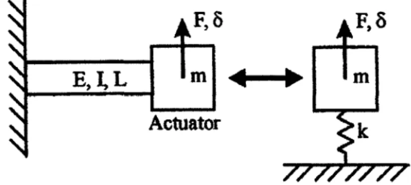
for the cantilever example. Figure 3.2 below shows the model for a first order flexure bearing. Some flexure bearings have more than one beam and so system can be modeled as a system of springs. One such flexure bearing that has multiple beams is the

HEXFLEX that will be further described in the next section.

F, 6

*F,

E, I, L

_{f M}

_I

_...

_{I M}

ActUator

_k

Figure 3.2: Spring model for actuator and flexure bearings

3.2 HEXFLEX

The HEXFLEX is a flexure based nano-positioner platform or bearing. Its design allows high resolution, repeatable and accurate 6 degrees of freedom motion [1]. An example of a HEXFLEX developed by Culpeper et al. is shown in figure 3.3. Figure 3.3 shows the resulting displacements for different actuator inputs. From the figure 3.3, it can be seen that a set of three actuators or actuator systems, capable of perfuming two-axis actuation is required for HEXFLEXes to attain 6 degrees of freedom motion. Section 3.4 below will talk about the final HEXFLEX that was adopted.

T1

F2

T3T

Figure3.3: HEXFLEX developed by Culpepper et al. showing example

displacements for give tab displacements. (x) shows direction into plane,

(0)

shows

directions out of plane, hollow arrows show actuator inputs and shaded arrows

show stage displacements

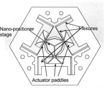
3.3 Final HEXFLEX design

The HEXFLEX design that is going to be used for the actuator system is largely

going to be designed to be compatible with sensors that are being developed by Robert

Panas [2]. Figure 3.4 shows the new HEXFLEX design. Because of this fact the

HEXFLEX design is already fixed and is described by Panas [2]. The work of this thesis

is going to concentrate on developing actuators that are compatible with the HEXFLEX

design developed by Panas

T1

T3P ₂

x T

0 0

Nano-po itio er

ex es

stage

0

0

0

0

Actuator paddles

CHAPTER

4

THERMAL CONSIDERATIONS- WAYS OF IMPROVING

THERMAL DISSIPATION

4.1 Printed circuit board design

The printed circuit boards (PCB) are used to as mechanical supports circuits. The PCB provide a much needed backing to keep electrical components fixed and allow for connections between the circuit components. Connections between components are maintained by copper traces that have different thickness. The copper thicknesses are rated in terms copper ounce weight per square foot. One oz. of copper corresponds to 1.4mils or 35.56 microns. In this project the PCB will only have traces and vias; no additional electrical components are needed for making the Lorenz coils described in chapter 2. The functional requirements for the PCB are:

* Mechanical support: Provide mechanical support for the traces both from external loads and internal loads. Internal loads coming from interaction of magnetic fields around each current carrying trace.

" Heat dissipation pathway: The PCB is also very important route for heat dissipation. Current passing through the traces cause heating up of the traces that could lead to damage in the PCB.

4.2 Thermal dissipation modes

The heat dissipation capability of the printed circuit board is very important for the safe and repeatable use of the actuators. There are three main ways that heat can be transferred away from the coils, namely conduction, radiation and convection.

4.2.1 Conduction

Conduction is the transfer of heat through solids and stationery fluids. This heat transfer is a result of particles (atoms, molecules and ions) being at different energetic levels. The more energetic particles will impact some other their energy to less energetic particles through direct interaction between the particles. Conduction mechanisms are different depending on the material properties of the substance and the phase of the

substance. In gases conduction is from random collisions between gases particles. Faster particles transfer some of their energy to slower particles that they collide with.

Conduction in liquids is similar to that of liquids but collisions are more frequent because particles are more densely packed in liquids than in gases. Solids have a different

mechanism since the atoms are in fixed positions. Heat is conducted through solids by means of lattice vibrations cause be atomic motion. Atoms at a higher temperature have high atomic motion and they pass on some of their energy to neighboring atoms. This interaction is more frequent that collisions in fluids and so solids tend to be better at conducting heat than the other phases.

Heat is conducted through matter only when there is a temperature gradient. Heat is conducted from a high temperature to a low temperature. For one dimensional

conduction heat transfer is described by the Fourier's law below:

q

k

where q "X is the heat flux, the heat energy being transferred in the x direction per unit area per unit time given in W/m2. is the temperature gradient, heat in the opposite direction of the gradient (hot to cold) and hence the negative sign in the equation. k is the thermal conductivity coefficient measured in Watts per meter-Kelvin (W/m.K). The thermal conductivity is a material property of the substance. For three dimensional heat conduction is given by the following equation:

Combining the above equation 4.2 and the first law of thermodynamic for an energy balance gives:

k + ak + k + . T 4.3

This equation is known as the heat equation. p is the density of the material in kilograms per cubic meter (kg/M3) and cp is the specific heat capacity of the material

with units of Joules per kilogram-Kelvin (J/kg.K). The right hand side of the equation represents rate of change in retained in a system [7]. The solution from the heat equation can be used to predict the thermal distribution of a material as a function of time. 4 is the rate at which heat is being generated within the system with units of Watts per unit volume (W/m3). Special note, the thermal conductivity can be directional for materials that are anisotropic. The heat equation is complicated to solve is normally simplified whenever possible by making suitable assumptions depending on the system.

Transient states of thermal conductions even though useful, will be left out in the thermal analysis of the printed circuit board (PCB) because the PCB is going to be designed to be able to survive long periods of time at max actuator force. The laminate

- I - - r.~ - - . - - ' - - - - I 1 .

used to make the board is going to be assumed to be isotropic even though there is a0-

slight directional dependence in the thermal conductivity value. Assuming steady state and isotopic material the heat equation above can be simplified to:

a2T + 2T + 2Tq

+1+ = 0 4.4

O X2 ay2 aZ2 k

The printed circuit board has a planar geometry meaning that the board thickness is much smaller compared to the length and the width of the board. The rate at which heat is transferred q is given by the following equation:

q = Aq" 4.5

This means that most of the heat is going to be transferred perpendicular to the face that is defined the length and the width of the plane because it has the greatest area compared to the other faces. Because heat generation4, only occurs in the coils it can be isolated to get an equation for the PCB that has zero heat generation. Equation 4.4 above can be reduced, by assuming one dimensional heat conduction and no heat generation to give:

-

k

0

dx dx or

___= 0 _4.7

dx

Therefore there is no change in heat flux in the direction on heat transfer.

4.2.2 Convection

Convection is a result of the motion of fluid particles and occurs from a surface to moving fluid. Convection is a mix of random fluid particle mixing (diffusion) and bulk motion of fluid particles (advection). The rate at which heat transferred by convection is given by the following equation:

q = hAs(Ts - Tco) 4.8

where q is the heat transferred rate in Watts. A, is the surface area that is exposed to convection in meters. T, and Tc, are the temperatures of the surface and the bulk

temperature of the fluid respectively. h is the convection coefficient in Watts per square meter-Kelvin (W/m2K). The convection coefficient depends is given by the following

equation:

Nu = 4.9

kf

where Nu is the Nusselt number, which is the ratio convectional heat transfer to fluid conduction heat transfer. The Nusselt number is a dimensionless number that depends on material properties of the fluid, geometry of the surface and the type of flow of fluid

across the surface. L is the characteristic length of the surface in meters. kf is the thermal conduction coefficient if the fluid in Watts per meter-Kelvin (W/m.K).

Convection heat transfer is going to be an important mechanism for carrying heat away from the surface of the PCB. Careful considerations the convective coefficient is going to be taken into consideration when designing the heat sink for the system.

4.2.3 Radiation

Thermal radiation results from oscillations and transitions of electrons between different energy states. These oscillations and transition result in atoms and molecules emitting energy in the form of electromagnetic waves. All forms of matter with a

of electromagnetic radiation no matter is required for heat transfer to occur. Radiation is mostly surface phenomenon except in the gases and semitransparent solids where is it a volumetric phenomenon. For the purposes of this thesis assume radiation as a surface phenomenon with the heat transfer given by:

q

where q is the rate at which heat is being transferred from the body in Watts. a is the Stefan-Boltzmann constant that is equal to 5.67x10-8

W.m-2K~4. T, and T are the temperatures of the surface of the body and the temperature of the environment respectively in Kelvins. A, is the surface area of the body in square meters. E is the thermal emissivity of the surface which is the ratio between the radiation energy emitted by a material to the radiation emitted by a black body. Since the temperature of the

surface of the PCB will not be significantly greater than the temperature of the surroundings heat transfer through radiation is going to be less that of the other heat transfer methods. Calculating the heat transfer through radiation is more complicated than the other types of heat because of the fact that it depends on surface properties of not only the PCB but includes those of the surroundings. Radiation heat transfer will not be

considered any further when analyzing the thermal properties of the actuator system because of its complexity to calculate and the fact that it is going to be smaller than the heat transferred to through other modes. Heat transfer through radiation is going to act as a safety buffer for the system, assuming that the surrounding temperatures are lower than those of the actuator system.

4.3Thermal resistance model

From equation 4.7 shows that heat flux traveling through a system is constant assuming one directional heat transfer. This means that at any particular cross-sectional area, that is perpendicular to the direction of heat transfer, the algebraic sum of the heat transfer to that area is equal to zero. This is similar to the circuit model for electricity where according to Kirchhoff's first law; the algebraic sum of current at a node is equal to zero. Applying the same model to thermal situations current will correspond to rate of heat transfer q and voltage will correspond to the temperature different across the body. In electrical circuits voltage and current are related by the following equation:

V = IR 4.11 where V is the voltage given in Volts and I is the current given in Amperes. R is the electrical resistance of the conductor and is given in Ohms. For the case of the heat transfer similar equation can be made since heat transfer rate is also directly propositional to the temperature different across the material. Therefore the corresponding equation for heat transfer is:

AT = q x R 4.12

where R is the thermal resistance of the material and has units of Watts per Kelvin. The lower the thermal resistance is the higher the heat transfer rate. The corresponding thermal resistances of conduction and convection heat transfer modes are shown below: Conduction R = 4.13 kA Convection R= 1 4.14 hA

These resistance values can be used in networks applying Kirchhoffs laws to calculate the heat flow or the steady state temperature the same way as they are used in electric

circuits [8]

4.4 Thermal Design for printed circuit boards

The printed circuit board (PCB) has to be designed in such a way that reduces the thermal resistance in the board. Almost all the heat transfer within the PCB is going to be through conduction. Looking at equation 4.13 above there are three ways to improve thermal heat through the material; 1) decrease the conduction length, 2) increase the area perpendicular to the conduction direction and 3) increase the thermal conduction of the material.

Analyzing at these options individually; decreasing the conduction length seems like one of the simplest one ways to decrease the thermal resistance but it has some complications of its own. In the case of PCB the conduction length for getting heat generated to the heat sink the thickness of the PCB. The conduction length is limited by PCB manufacturing capabilities. The standard PCB has a finished thickness of

0.062inches or 1.57milimeters but the thickness of PCBs can vary from as small as 0.010inches to 0.250inches or 0.254milimeters to 6.35milimeters [9]. Picking one of smallest thickness is the best way to reduce the thermal resistance since thermal resistance is directly proportional to the conductive length. Purchasing these thin PCBs can be very expensive because producing thin PCBs requires special equipment and is not supported by all the PCB manufacturers. This means that there is a tradeoff between cost and thermal performance. The reduction in the thickness of the PCB means a

decrease in the mechanical strength of the PCB but this should not be a major issue since the attachment of the PCB to a heat sink will provide more than the needed mechanical support.

Increasing the area perpendicular to the direction of heat transfer can be achieved either spreading the heat dissipating elements over the area of the board or spreading the heat dissipated by these elements cross that plane of the PCB board through in plane conduction. Spreading dissipative elements over the surface of the PCB is not ideal for this case because the coils have to be located in a specific area to maximize the force that they generate. The latter option spreading the dissipative heat through in plane

conduction is the most practical in this case. This is achieved by reducing the in plane thermal resistance, allowing the heat to spread over a wide area before it is finally conducted along the thickness of the PCB to the heat sink.

The last means of decreasing the thermal resistance of the PCB is by increasing the thermal conductive coefficient of the PCB. There is a limitation on the type of materials that can be used in making PCB boards. This constraint is based on both the functional requirements of PCBs and on what materials PCB manufactures typically use to make PCBs. The main material used in making PCBs is the laminate material than it used to keep components in a fixed position relative to each other while making sure that the components electrically insulated from each other. Other materials can be added to the laminate that can be used to improve the thermal conductivity of the PCB. One material that is easily added to the laminate to improve the thermal conductive properties of the PCB is copper since it has a high thermal conductivity. Copper can be introduced into the laminate by adding copper elements that do not have that do not have any

functions in the electrical circuit like copper pours that will be discussed in section 4.5.2 below.

4.4.1 Printed circuit laminate

PCB manufactures support making PCBs from a number of materials but FR-4 is by far the most common and widely used. For purposes of this work we are going to restrict PCB material to just FR-4 because it reliability and low cost to make into PCBs. FR-4 has a thermal conductivity of 0.25W/m-K, which is significantly than the thermal conductivity of copper of 335W/m-K. So adding copper features to FR-4 greatly improves the heat transfer of the PCBs.

4.4.2 Copper Pour

As mentioned in section 4.5.1 above copper has a thermal conductive that is 3 orders of magnitude greater than that of FR-4, which is the material that the laminate is made from. One simple way of adding copper to the PCBs is incorporating copper pours

into the board design. Copper pours are polygon shapes that are filled with copper that can be added to circuit boards to improve thermal conductivity. Copper pours are in the same plane as electrical traces and so help with spreading the heat across the plane. Copper pours, like electrical traces, do not go between different planes and so have a greater impact on in plane thermal conduction as opposed to thermal conduction along the thickness of the PCB. The thickness of the copper pour is that same as the thickness of the electrical traces

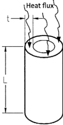
4.4.3 Thermal Vias

Thermal vias, shown in figure 4.1 below, unlike copper pours cross different planes in PCBs. This makes them very important increasing thermal conductivity along the thickness of the PCB. Vias are holes that go through PCBs. Vias can be either plated

with copper or non-plated. Plated vias are used for either forming electrical connections between traces in different layers or as thermal vias where the vias are not electrically connected to anything and are there for the sole purpose of improving thermal conductivity. The effectiveness of thermal vias is increased mostly by increasing the

plating (barrel) thickness and decreasing the spacing between adjacent vias allowing for more thermal vias to be put onto the via [10]

Heat flux

L

Figure 4.1: Heat transfer via the copper walls of a thermal via

Since thermal vias are just holes through the PCB there is a possibility of making them more conductive by filling them up with solder or adding other conductive material like copper posts. This thesis will look into the possibility of sticking copper posts into thermal vias; copper posts have a thermal conductivity that is almost 10times as large as that of regular solder. Thermal grease can be used to decrease the contact resistance between the copper posts and the vias to a negligible level. The result is an increase effective conductivity of the via that will be analyzed in section 5.3

CHAPTER

5

SIMULATIONS AND DESIGN OPTIMIZATION

Stress-strain, electromagnetic and thermal simulations were conducted to determine the feasibility of the design.

5.1 Flexure/HEXFLEX Simulation

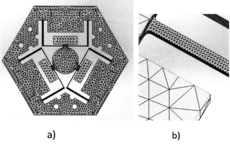
Finite Element Analysis (FEA) simulations, using Solidworks, were conducted on the HEXFLEX to determine the forces that the actuators must provide to allow for ±20pm translation allow along all three axes. A mesh was applied to the model with a control mesh being applied to the flexures to account for their smaller dimension in comparison to the rest of the model. Figure 5.1a) below shows the mesh for the whole HEXFLEX and Figure 5.lb) below shows the comparison between regular mesh area and area where mesh control was applied.

a)

b)

Figure 5.1: a) General meshing used for the simulation. b) local mesh control

applied to flexures to improve simulation accuracy

Figures 5.2and

5.3

below show the results of the simulations for in plane and out of plane

actuation. The three out of plane actuators need to each provide 0.12N to provide the

required maximum displacement. In plane actuators on the other hand need to provide

0.17N to achieve the required maximum displacement. In all these cases the maximum

stress of the flexure has been below

5%

of the yield stress of titanium, which means that

the bearing is not being over stressed. Table 5.1 summarizes the results from the

-td Ic nr MCNA

Study nam Sty 3 .E

Plot typ& Static d scen Displacamer gai ff

Del orratm scale:45 _,94d

2 O94e-002 1.920e-002 1.745102 .t.57e-002 .1.396e41(2 .1.222e-002 .047e-22 .8.72Ge-003 52ste4m0 3.490e-M3 1,745e-(3 1.0000-03M

Figure 5.2: In plane actuation of HEXFLEX with 0.17N applied to two of the paddles. Arrows show the direction in which the forces are applied.

W',~ nin MCtuA SW*uny FSud 2

Plo 1), StatC _u..r , , uri Deforfftai ... 241,775 LRS (wan) SAMe-C2 1.7230-,2 . 3490-M0 .6.8930M1 5.1700-M0 13.4478-=0 1.7235-003 D18002

Figure 5.3: Out

three paddles.

of plane actuation of HEXFLEX with 0.12N applied to normal to all

Table 5.1: Results from flexure simulation

Actuator

Force (N)

displacement (pm)

In-plane (z-axis)

0.12

21

5.2 EM simulation

The system actuators work off interactions between electrical and magnetic fields, as described in section 2. The Lorentz coil forces can be calculated using the equations 2.1 and 2.2. The simulation of the forces generated by these coils was developed by Golda [5]. In the simulation Fourier transform model and trapezoidal numerical methods are used to compute the field generated by the permanent magnets. Coil segments are broken up into segments by an algorithm and equations 2.1 and 2.2 are applied to these

equations to calculate the force and moment on each segment. The total Lorentz force on the coils is calculated by summing up all the forces on all the segments. The total

moment force is calculated by summing up all moments on all the segments and summing up all the moments contributed by forces on each segment.

5.2.1 Simulation parameters

Simulations were ran to determine the how the force generated by Lorentz coils varied. Looking at equation 2.1 the force output is directly proportional to the amount of current that flows through the coils. At the same it the more current that passes through the coil the higher the Joule heating that is given by the equation below:

q = i2 R 5.1

Where q is the dissipated heat, i is the current flowing through the coils, and R is the total electrical resistance of the coils. Therefore heat dissipated is directly proportional to the square of the current, whereas the force output is only directly proportional to current as shown in equation 2.1. This means increasing current will result in a greater change in the heat dissipated than the change in force output. Simulations were conducted on both in plane actuator(X-actuator) and out of plane actuator (Z-actuator) Table 5.1 below is the list of parameters that can be varied in the actuator design

Table 5.2: Parameters for Lorentz coils simulation

Parameter

Current

nL

Simulations were run to determine following default values should be

Value

Copper weight or trace thickness width of coil

maximum current density(0.001 for copper) current through the coils

spacing between coil windings width of magnet

Remnance

height of coils above surface of magnets number of integration point=1000

the effects of varying these parameters but the assumed unless otherwise noted.

Table 5.3: Standard simulation values

Parameter

Jmax

Value

2oz copper per square ft 300pm 0.00lA/pm2 5A 144pm +bcoil* 3.175mm 1.25T 120pm

1000

*There has to be a minimum spacing of 144pm needed between 2oz copper traces

5.2.2 Simulation results and analysis

The simulations were run and the results are shown in figures 5.4to figure 5.6

the force output. Figure 5.4 _{shows that the force output decreases as the width of the coil}

increases, while the percentage error from parasitic forces also increases. Increase in coil width results in a decrease in the number of coil turns which also leads to less force being generated. The increase in parasitic forces could be attributed to the fact that as the coils get wider there are some sections of the coil that will end up in regions that don't have uniform magnet fields. On other hand as the coil width increases there is a drop in power dissipated by the coils because the resistance of the coils is inversely proportional to coil width. The drop in resistance means more current can be carried for the same power generation

I

~~~.

Figure

5.4:

_{Results for X-Actuator simulation Ftotalx vs. bcoil including variation}

in parasitic force error as a percentage of Ftotalx. This graph is similar to the one

for Ftotalz vs. bcoil.

Figure

5.5

_{below shows that as the force output of the coils decreases as copper}

weight increases. This could be attributed to the fact that as copper weight increases there

is a drop in the current density in the coils (current per unit cross-sectional area). The

drop in current density could lead to weaker interactions between the magnetic field and

the moving charges. On the other hand, like the case with increasing coil width,

increasing copper weight will result in a decrease in the power dissipated. Copper

thickness is also inversely proportional to resistance.

i

0.04

I

Figure

5.5:

Results for Z-Actuator simulation Ftotalz vs. tcoilCuweight including

variation in parasitic force error as a percentage of Ftotalz. This graph is similar

to the one for Ftotalx vs. tcoilCuweight.

Figure

5.6

below shows that force output increases linearly with increasing

current. This is predicted from equation 2.1, that force output is directly proportional to

current. There doesn't seem to be a clear trend in the variation of the percentage error.

The variation the force error very small, it only changes by about 0.07% meaning that it

can be assumed that percentage force error does not depend on current.

£ £ -- ~~8~ 0 4 0 0 ---0.3 1.86 0.15 L82J 0.1 £ % error 8 £ £ ~ 0 1.78 1.84 1.81 1.82 1.9~ 0.25 0.2 0.5

I

I

I

1..

i

Figure

5.6:

Results for Z-Actuator simulation Ftotal_.z vs. Current including

variation in parasitic force error as a percentage of Ftotal_z. This graph is similar to

the one for Ftotalx vs. Current.

Figure

5.7

below shows that the force out is directly proportional to the negative

of height the coils above the surface of the magnets. This linear relationship force output

to height has an R-squared value of almost 0.99. This relationship results from the fact

that the magnetic field decreases linear for distances that are less than its characteristic

length. In this case the characteristic length of the magnet, al, is 3.175mm so this

approximation is safe to assume for distance around 10% of this value [5].

*tota Lz

16

toAA 0. 16 0.14 0.i1a Oa0. p0.08 0.06

~:

-* -n"Ot

Figure 5.7 :Results for Z-Actuator simulation Ftotal_z vs. height of coils above

magnet surface above including variation in parasitic force error as a percentage of

Ftotalz with Current=8A. This graph is similar to the one for Ftotalx vs. Height.

5.2.3 Summary of results

The force and power dissipated by the coils is depends on a number of parameters

as described in table 5.1. Careful selection of these parameters to maximize force and

minimize heat dissipation is required. Also the maximum parasitic force error from the

simulations has been less than 5% error, which is good. After considering the plots above

the following parameters show in table 5.2 were chosen. Table 5.3 shows the force

values, required current and the power dissipated for this configuration

Table 5.4 Summary of simulation results

Force required

Power dissipated

Actuator type

()Current

(A)(W

(N) (W)

X-actuator

0.173

7

6.28

Z-actuator

0.120

8

4.22

From table 5.3 It can be seen that the total power dissipated is going to be 10.50W. A

value of 11W was used for the thermal simulations.

DO * Ftotauz-% %error Linear (Ftotal_.) 2 0.5 0 ) 100 2 500 600 700

5.3 Thermal simulation

Thermal simulation was conducted on a 0.5in by 1.5in PCB to determine the effects of adding thermal vias with copper posts stuck in them. As described in section 4.5.3 the introduction of copper post should decrease the effective thermal resistance of the PCB. The PCB is going to be a four-layer board with the coils being on two of these layers. The other two layers as a route to get current out of the middle of the coils. The PCB model consists of four alternating layers of laminate made out of FR-4 and copper layers. Two of the copper layers contain the heat dissipating coils surrounded by copper pour and the other two layers are layers of copper. These layers are stacked on top of each other with a laminate layer being at the bottom and a copper layer at the top of the PCB. The thickness of the copper layers is 2oz copper per square foot or 71.12 microns. The thickness of the laminates depends on overall thickness of the PCB. PCBs with overall thickness of 0.787mm and 1.575 have laminates of thickness of 0.125mm and 0.323mm, respectively. The bottom of the PCB will also have a copper plate that will model heat sink attached to the system.

Thermal contact resistance is assumed to be negligible between within the model. This is a fair assumption considering that FR-4 has a high thermal resistance and will most probably contribute more to the resistance of the system than contact resistance. The thermal interaction between the copper pour and coil is modeled as a distributed thermal resistance of 0.608x10 K-m2 /W due to the fact that there is a thin layer of laminate,

about 0.152mm thick, that provides electrical insulation between the copper pour and the coil.

Thermal inputs into the system include 5.5W dissipation from each coil producing a total 11W, which corresponds to the value found in section 5.2. Convection heat

transfer assumed to occur at both the top face of the PCB, and at the bottom of the "heat sink" plate attach to bottom of the PCB. The top of the PCB has a convective coefficient of 10W/M2 -K, which conservative estimate of free convection [7] and the "heat sink" has a convective heat transfer coefficient of 1000W/m2_{-K, which is an achievable value for}

an active convection coefficient and fins combination, attached to the "heat sink". Ambient temperature is assumed to be 298K.

The PCB also includes 14 holes where a varying number of thermal vias/copper post can be introduced into the PCB. The holes have a diameter of 0.6mm. The holes are on either side of where the copper coils are as shown in figure 5.8 below.

Figure

5.8:

Holes used to allow the introduction of copper posts into the PCB.

A thermal simulation was run in Solidworks to determine the steady state

temperature. Figure

5.9

below shows the thermal chart of the results of one of the

simulation.

There is higher temperature for the zone over the coils. Figure 5.10 below also shows that the highest temperatures occur along the sides of the PCB board that don't have the copper posts. Adding copper posts to the sides will also improve the thermal performance.

Figure 5.10: The highest temperature occurs along the sides that do not have copper

posts and these points along the same plane as the coils.

The results from the simulation are shown the figure 5.11 below is for the

1.575mm PCB. The maximum final temperature decreases as more and more posts are

introduce into the PCB. The maximum operating temperature of FR-4 is 413K. Without

the copper posts the PCB would over heat and fail.