Design of observers for the swing dynamics of power networks

Design of Observers for the Swing Dynamics of Power

Networks

by

Paisarn Sonthikorn

Submitted to the Department of Electrical Engineering and Computer Science

in partial fulfillment of the requirements for the degree of

Master of Engineering in Electrical Engineering and Computer Science

at the

MASSACHUSETTS INSTITUTE OF TECHNOLOGY

May 2002

@

Massachusetts Institute of Technology 2002. All rights reserved.

A uthor ...

Department of Electrical Engineering and Computer Science

May 24, 2002

Certified by ...

Accepted by ...

George C. Verghese

Professor of Electrical Engineering

Thesis Supervisor

Arthur C. Smith

Chairman, Department Committee on Graduate Students

MASSACHUSETTS INSTITUTE OFTECHNOLOGY

Design of Observers for the Swing Dynamics of Power Networks

by

Paisarn Sonthikorn

Submitted to the Department of Electrical Engineering and Computer Science on May 24, 2002, in partial fulfillment of the

requirements for the degree of

Master of Engineering in Electrical Engineering and Computer Science

Abstract

This thesis presents a design of swing-state power network observers. The network observer concept is motivated by researchers' attempt to better understand complex interactions of power networks in order to achieve efficient fault monitoring processes. Based on the nonlin-ear DAE swing model and the nonlinnonlin-ear measurement model, the network observer has its gain computed by using the Linear Quadratic Estimator (LQE) method. Using the classical nine-bus system as a test system and having two representative system disturbances: a line drop and a change in power injection at a load node, numerical studies of the observer shows impressive results in terms of both fast convergence rate and low offsets between the real state values and predicted ones. The underline reasoning behind the network observer good performance is that, by using a highly nonredundant set of sensors, this network observer can exploit its inherited nonlinear models to accumulate over time and to interpolate over space in order to generate satisfactory numerical state predictions. Later, Two fault isola-tion methods using the network observer: multiple observer scheme and nominal observer scheme, give us good results and provide insights into the effect of the disturbances on the network behaviors.

Thesis Supervisor: George C. Verghese Title: Professor of Electrical Engineering

Acknowledgments

I am deeply thankful to Professor George C. Verghese, my great mentor, who has stimulated my research interest and has provided invaluable advice to me all along my M.Eng. year at MIT.

Thanks to Associate Professor Bernard Lesieutre, my supportive and friendly ex-academic advisor, for your guide and encouragement.

Thanks to Ernst Scholtz for all your supports, help and understanding in both research and psychological issues.

Thanks to Joshua W. Phinney for his technical advice on LATEX.

Thanks to Vivian Mizuno for all the help she has provided me all along.

Many thanks to P'Teng (Poompat Saengudomlert) and P'Yong (Watjana Lilaonitkul) for your consistent supports.

Thanks to my oldest brother, Paiboon Sonthikorn, I am deeply in debt to your guidances. Thanks to my cheerful older sister, Ratchanee Sonthikorn, for keeping my world bright and joyful. Thanks to my older brother, Paitoon Sonthikorn, for always making me realize how to stay strong in this world. And thanks to my little sister, Nong Pond (Thanawan Kittisuwan), for cheering me up every time I am desperated and doomed.

Forever thanks to my Mom, Saovaluck Sonthikorn, and my Dad, Jane Sonthikorn, for having nurtured me to be a good person, and for always being proud of who I am. Being your son is a blessing from Heaven!

Thanks to the people of the Kingdom of Thailand for giving me all these opportunities; I hope to prove your tax money worthwhile!

Thanks also to the Electric Power Research Institute (EPRI) and the Department of Defense (DoD) for partial support of my research.

... Here I am, at the Massachusetts Institute of Technology, which used to be my dream school and has been such a great institute that will shape my life forever.

Contents

1 Introduction

1.1 Motivations for Network Observers . . . . 1.2 Term inology . . . .

2 Modeling for Observer Design

2.1 Nonlinear Swing Model . . . . 2.2 Nonlinear Measurement equations . . . . 2.3 Linearizing the Swing and Measurement Models . . . . 2.3.1 Linearizing the Swing Model . . . . 2.3.2 Linearizing the Measurement Models . . . . 2.4 Collapsing the Linearized Swing Model . . . . 2.5 Observer Design Methodology . . . . 2.5.1 Linear Observer for Linearized State-Space Swing Model . 2.5.2 Nonlinear Observer for Nonlinear DAE Swing Model . . .

3 Numerical Results of Observer Studies

3.1 The Observer in Action . . . . 3.2 Selecting the

Q

and R Matrices . . . . 3.3 Types of Measurement and Placement . . . .

3.4 Pole Placement VS LQE . . . .

4 Fault Isolation Applications

4.1 Multiple Observers for Fault Isolation . . . . 4.2 Understanding Faults on the Network: Line Parameter 4.2.1 Normal Operation . . . . Disturbances 9 10 11 12 . . . . 12 . . . . 14 . . . . 15 . . . . 15 . . . . 16 . . . . 17 . . . . 18 . . . . 18 . . . . 19 21 . . . . 22 . . . . 25 . . . . 27 . . . . 28 32 . . . . 32 . . . . 35 . . . . 36

4.2.2 Investigation of the Steady-State Output Error Vectors . . . . 36

4.2.3 Gaining Insights into ey Vectors . . . . 40

4.2.4 Achieving Fault Isolation via a Nominal Network Observer . . . . . 42

4.3 Analysis of Steady-State Output Error Vectors . . . . 45

4.3.1 Discussion about the Analysis . . . . 46

4.3.2 Numerical Results of the Analysis . . . . 47

4.3.3 Exploring on the Nonlinear DAE Swing Model: Complement Tool For Fault Isolation . . . . 47

4.4 Sum m ary . . . . 49

5 Summary 50 5.1 Brief Content Overview . . . . 50

5.2 Suggestions for Future Studies . . . . 51

List of Figures

3-1 Classical 9-bus example studied in this paper. The line parameters are shown as im pedances. . . . . 22 3-2 Time plots of 64-61 (system) and 64-61 (observer) when Event 1 occurred

(beginning at t =0.1s, duration 3s). . . . . 23 3-3 Time plots of 65-61 (system) and 65-61 (observer) when Event 1 occurred

(beginning at t = 0.1s, duration 3s). . . . . 24 3-4 Time plots of w3 (system) and &3 (observer) when Event 1 occurred

(begin-ning at t = 0.1s, duration 3s). . . . . 24 3-5 Time plots of 6₃-61 (system) and 63-61 (observer) when Event 2 occurred

(beginning at t = 0.1s, duration 3s). . . . . 25 3-6 Time plots of 64-61 (system) and S4-61 (observer) when Event 2 occurred

(beginning at t = 0.1s, duration 3s). . . . . 26 3-7 Time plots of 66-61 (system) and 66-61 (observer) when Event 2 occurred

(beginning at t = 0.1s, duration 3s). . . . . 26 3-8 Time plots of 64-61 (plant), Sso-61 (suboptimal) and S4'0-61 (worst case

com-panion) when "event 1" occurred (beginning at t =

0.1s

duration 3s). . . 28

3-9 Time plots of 62-61 (system) and 62-61 (for both LQE observer and pole-placement observer) when Event 1 occurred (beginning at t =

0.1s,

duration

3 s ) . . . . . 29

3-10 Time plots of 67-61 (system) and 67-61 (for both LQE observer and pole-placement observer) when Event 1 occurred (beginning at t = 0.1s, duration

3 s ). . . . . 30

3-11 Time plots of w6 (system) and C.,6 (for both LQE observer and pole-placement

3-12 Time plots of 64-61 (system) and

54-

1 (for both LQE observer and

pole-placement observer) when Event 1 occurred (beginning at t =

0.1s,

duration

3s)... ... 31

4-1 Time plots of the residuals (65-61) - (65-61) of different observers when the

real system has Line 9 taken out. . . . . 34 4-2 Time plots of the residuals (4-61) - (₆ -6₁) of different observers when the

real system has Line 9 taken out... ... 34 4-3 Time plots of the residuals (68-61) - (68-61) of different observers when the

real system has Line 9 taken out. . . . . 35 4-4 Normal operation of the classical 9-bus sytem: angles and power flows. . . . 37 4-5 Steady-state output error plot of all six simulations. . . . . 38 4-6 EY vector plot of all six simulations with all the line parameters perturbed

within five percent of the original values. . . . . 39 4-7 iy vector plot of all six simulations with all the line parameters perturbed

within ten percent of the original values. . . . . 40 4-8 ey vector plot of all six simulations with all power injections and extractions

perturbed roughly by ten percent. . . . . 41 4-9 Steady-state after Line 4 getting cut off from classical 9-bus sytem: angles

List of Tables

4.1 The measurement errors for all three sensors of the observers when there is no line or power variation. . . . . 41 4.2 The direction of

ey

vectors of the previous four studies. . . . . 44 4.3 The magnitude changes of Ey vectors of all the studies. . . . . 45

Chapter 1

Introduction

The concept of state estimators or observers has been prevalent in the control theory area. However, there has not been sufficient study of its application to the swing dynamics of power systems. This thesis has the objective of discovering more about power network observers in terms of design concepts and later providing application examples in fault isolation as supporting evidence that the design can achieve promising results.

This thesis shows how to approach dynamic real-time swing-state estimation for power networks using observer design. The study in this thesis has been developed and expanded from that in

[1]

to have more types of sensors and to allow the network to include load buses (or "buses"). The network observer design methodology we developed utilizes three important components to achieve good state estimates: observer gain based on linearized and collapsed swing models, with the standard Linear Quadratic Estimator (LQE) technique applied; a nonlinear DAE (differential-algebraic equation) swing model as the inherited model of the observer; and the freedom to use four possible measurement types for observer's inputs: a bus angle, a speed deviation from synchronous associated with generator, a net power at bus flowing into the network and a power flow on a tranmission line.

Based on the classical nine-bus network in [2] as a test system, we can have the model-based observer, as will be shown, generate good numerical state predictions by using the information that the nonlinear model of the observer accumulates over time and interpolates over space from the measurements of a highly non-redundant set of sensors. The classical nine-bus example helps illustrate our results and explore how performance varies with the number, nature, and placement of measurements. Although still needing further

investiga-tions, comparative simulations with an observer using a heuristic gain shows that an LQE observer can achieve good predictions with a fast convergence rate and low residuals.

Next, we briefly investigate possible application of our network observer in fault detec-tion and diagnosis. First, a multiple observer scheme [3] is introduced and implemented using our observers. Then we examine a possibility of using the steady-state output error (

y)

vectors resulting from complete single line-out faults to achieve fault isolation. After that we do analyses to gain insights into the relation between faults and their corresponding

ey vectors.

Chapter 2 describes the modeling and design methodology of our network observer. Chapter 3 presents the numerical results of our observer by using the classical nine-bus system as a test system and also briefly shows performance comparison study between our LQE observer with a pole-placement observer.

Chapter 4 provides a few examples in the fault isolation application of the network observer.

Chapter 5 offers the conclusion of this thesis and suggests possible future studies.

1.1

Motivations for Network Observers

Large interconnected networks, such as power grids, communication networks, and the In-ternet, sometimes suffer from cascading outages [6]. To prevent future blackouts, it is essential to understand such networks' dynamic behavior and relate it to their underly-ing network structures. At MIT's Laboratory for Electromagnetic and Electronic Systems (LEES), researchers are examining relationships between the graph of a power network (i.e., the topology of the network) and the dynamic properties of the system. Here one important issue is the monitoring of power systems after faults or disturbances. These disturbances generally give rise to oscillating modal components, which in a worst-case scenario can go unstable. Such a phenomenon can pose a serious problem to system reliability if not detected and damped out.

The concept of network observers then becomes a crucial element in determining the evolution of network states. By better understanding the network behaviors both before and after disturbances, we can then design and generate appropriate counteractions against possible threats from faults. Eventually, we want our network observer to be robust and

informative in predicting the states of huge and complex networks in order to help re-searchers to better understand the complicated evolution of the network characteristics both electrically and topologically. Thus, we can have a solid foundation to build effective fault detection and diagnosis schemes for real world systems.

1.2

Terminology

Fault Monitoring Process: The terminology of the monitoring process can be confusing

since there is no standard. Here, we want to provide definitions from

[4],

which are used throughout this thesis.

" Fault detection answers the question - Has a fault occured?

" Fault identification answers the question - Which observation variables should we identify as most relevant to diagnosing the fault?

" Fault diagnosis answers the questions - Which fault occured? What is the cause of it? And what is the type, magnitude and time of the fault?

" Fault isolation answers the question - Where exactly in the network is the faulty component?

In this thesis, we focus on studying the application of our network observer mostly to fault isolation, i.e., determine which component is faulty. Throughout Chapter 4, we assume that the faults of interest are complete single line-out faults; what we are trying to achieve is determining which line is cut.

Distinction between Parameter Estimation and Observer-Based Method: Both are

fun-damental analytical methods in various engineering fields. However, the reader should understand clearly the distinction between the two since they are similar in some aspects and might cause some confusion if one wanted to proceed in the parameter estimation di-rection. And though they are two different methods, one can certainly combine the two to do the fault monitoring process. It is noted that the focus of this thesis is the observer-based method. We advise the reader to refer to [5] to familiarize himself or herself with the concepts of both methods. Also, [6] provides discussions about the combination of the two analytical methods.

Chapter 2

Modeling for Observer Design

In this chapter, the nonlinear swing model that is the basis for our network observer is first presented. Next, we show the nonlinear models for different types of measurements: bus angles, generator speeds, line power flows, and power injected into or extracted from buses. By linearizing and collapsing the nonlinear models, we can then construct a linear observer for the linear state-space swing model. Using the linear gain computed via the LQE method, we can integrate it with the nonlinear models to create a nonlinear observer, which is the network observer we will use throughout this thesis.

2.1

Nonlinear Swing Model

Throughout this thesis, we use the nonlinear swing model to understand the behavior of the power network. Also, this model is a crucial part of our observer design since it is the knowledge base of our observer in understanding the electromechanical behaviors of the network. Therefore, this section intends to help the reader understand the details of the model and the notations of its associated elements.

It is noted that, for the power systems of our study, we assume that the voltage magni-tudes of the network are tightly controlled around 1 p.u., so we take them all to have this value. Let 6 denote the vector of bus angles, and P(6) denote the real power flowing into the network, so

where: 1) F is the directed bus-line incidence matrix of the network graph (the orientation of line h can be picked arbitrarily, and F,,h = -1, Ft,h 1 if this directed line goes from bus s to bus

t);

2) ' denotes matrix transposition;

3) Depending on the context, diag(-) extracts the diagonal of its matrix argument and forms a column vector, or forms a diagonal matrix by placing its vector argument on the diagonal;

4) sin(.) and cos(.) imply taking elementwise sine or cosine of the corresponding vector arguments;

5) B and

g

are diagonal matrices with line susceptances and conductances as diagonal elements.

Throughout this thesis all vectors are typically ordered as:

(

=

[

' '', where sub-scripts g and I indicate generator and load buses. For examples, =

[

6'

1 ,5' '. However, it is noted that we define the speed vector as w =

[2]'

because we are only interested in determining the speed of generators.

We also define the following: n is the total number of buses in the system; ng, is the number of generator buses; and n, = n -

n

is the number of load buses. We note that

F'6 yields a vector of angle differences across branches of the network; diag(FgF') is an

n-dimensional vector whose elements are the sums of the conductances of lines emanating from the corresponding buses.

Using (2.1) we can then construct the nonlinear DAE swing model as follows:

M i f(x,u,w)

1 0 0

0 0 0

1=1

pe P (6) (2.2)

0 0 Mg pe - P9(6) - Dgw

where 6g, 61, and w are respectively the generator angles, load angles, and generator speed deviations from synchronous speed. We use x to denote these internal variables of the DAE description. Note that 6g and w are state or differential variables, while 61 comprises alge-braic variables. The vector PFe denotes power injected at the load buses (and hence typically has negative entries), while Pg is the net power injected at the generator buses (typically

mechanical power input to a generator minus the local real-power load)1. Integrating these two vectors, we define Pe as the vector of external bus power injections. These injections may be partly or completely known; the known parts are gathered in the vector u, while the unknown parts "process noise" are gathered in w (i.e., implicitly we have Pe - + w).

D9 and Mg are diagonal matrices whose nonzero entries respectively comprise the damping

coefficients and the (normalized) inertias of the generators. Discussion: The second and the third rows of the nonlinear DAE swing model in (2.2) provide a useful framework on the network behaviors2. The second row tells us that Pe = P (6), which means that the power

extractions at the load buses equal the power flow from the network into those buses. The last row is essentially the swing equation3_{, which characterizes the behaviors of the power} at the generator buses.

2.2

Nonlinear Measurement equations

Here, we present the nonlinear measurement models characterizing outputs as nonlinear fuctions of its corresponding inputs. This thesis allows four possible types of measurements. The ith measurement can be

I

j if j E{, - , n} =i _if j _{E {1,... n}}

(2.3)

Pj (6) if j C{1, , n}

Pst (6) if s,tiE III, - n}

where 6j is the bus angle associated with bus

j,

wj is the speed deviation from synchronous

speed associated with generator

j,

P (6) is the net power at bus

j

flowing into the network (this is simply the Jth element of (2.1)) and Pt(6) is the power injected at s onto the line h that connects to bus t. To obtain an explicit expression for this latter measurement, note

'It is noted that the net power injected at the generator buses can vary because although the mechanical power has to stay the same, the local real-power load can shift to another steady-state value due to any event happening to the system. However, if there is no direct change in load extraction, Pf needs to maintain its steady-state value.

2

The first row just says that

S9

= W. This row, though not informative, helps us obtain a matrix form of

the swing model.

3

first that the vector of flows Pine(6) on the lines of the network can be expressed as

1

Pi, e(6) = B sin(F'6) -g cos(F'6) - -g(F' - F1') (2.4)

2

If the orientation picked for line h when defining F goes from bus s to bus t, then Pot(6) in (2.3) is simply the hth component of Pie() above.

Gathering all the available measurements into a vector y, we obtain a vector measure-ment equation of the form

y = g(x) + v (2.5)

where x is as defined earlier, and v denotes a vector of sensor or measurement noise variables.

2.3

Linearizing the Swing and Measurement Models

In order to use standard state-space observer design techniques, we will work with small-signal versions of the nonlinear swing model and the measurement equations, linearized

around steady-state. Note that a vector in the nonlinear system can be expressed as

((t)

=

(* + ((t),

where (* is the steady-state vector and

((t)

is the vector of deviations from this steady-state, assumed small when deriving the linearized model. In order to simplify notation, we will suppress the time dependence of the variables.

2.3.1 Linearizing the Swing Model

We linearize the nonlinear DAE swing model (2.2) around the steady state (loadflow) so-lution

6

6*

and w =

w*

=

0.

Evaluating the Jacobian a = K (where K is

referred to as the spring or synchronizing matrix of the system), one finds the following:

K = -FL3diag(cos(F'6*))F' + \F|gdiag(sin(FJ* ))F' (2.6)

From (2.6), we can partition K into four submatrices, Kgg, KI, Kig and K1, as follows:

K= K9g K9, (2.7)

where K_{9g E 7Z9"g is a spring matrix associated with transmission lines connecting a}

generator to another generator; Ki E

R"

""' is a spring matrix associated with transmission lines connecting a load to another load; Kg E Xfl"' is a spring matrix associated with

transmission lines connecting a load to a generator, and K = K'1. It is worth noting

that K is positive semidefinite and has a Laplacian structure, which has the property that

Neglecting higher-order terms of A in the linearization of (2.2), we obtain a linearized DAE swing model of the form:

A G

10 0 0 0 I A69 0

0 0 0 -K₁₉ -Ku 0 A6

+

G

Ape (2.8)

0 0 M -K -K 9 1 -D

j

Aw G

2.3.2 Linearizing the Measurement Models

Linearizing (2.5) results in an expression of the form

Ay = CAX + Av. (2.9)

where C =

[-1

Any available angle and speed measurements are already linear functions of x, so their contributions to (2.9) are clear on inspection. For measurements of bus power injection

P (6), the linearization is simply yielded by the corresponding row of the Jacobian K. For

measurements of line power flow, we similarly pick the appropriate rows of the linearization

of Pine() (

[]

_66, = E)

E = 3diag(cos(F'S*))F' + diag(cos(F'3*))F'. (2.10)

Thus C in (2.9) is constructed by gathering a selection of rows from each of the following

matrices:

[

Inxn 0

]

(direct angle measurements);

[

Ong xn Ing x n, ] (generator speed

mea-surements);

[

K

Onxn,

]

(bus power injection measurements);

[

E

Onxn,

] (line power flow measurements).

obtaining a state-space swing model for our observer design. The reason is that we want to mutiply the inverse of the leftmost matrix to both sides to achieve a state-space swing model; however, the diagonal matrix has zero diagonal elements, which implies that the matrix itself is singular. The structure of the matrix results from our networks having both loads and generators. Therefore, we need to another step that can get around the problem, but can still maintain all the state information.

2.4

Collapsing the Linearized Swing Model

To form a state-space swing model that can be used for our observer design, we execute a Ward-type reduction on the linearized DAE swing model (2.8). This will help us suppress the problem that we had in the previous section, i.e., expressing the load angles as a function of the generator angles. However, a crucial assumption for this reduction is that K₁ is invertible, and this is generally the case for our systems of study (implying that the DAE model is of index 1). From (2.8) the relationship between load angles and generator angles is found to be

A61 = -Kij 1(Kj9A6 S- GIAPFe). (2.11)

Substituting (2.11) back into (2.8) and defining

A

Ke = Kgg - KgiKj Kig (2.12)

Gc = Gg - K9iKIj Gi (2.13)

and S = -M- 1, the collapsed all-generator linearized state-space swing model is expressed as:

A x

og0 I A69 0e

+ - AP. (2.14)

The driving term in the above equation can be written as the sum BAu + GAw, where

a

and w are as defined earlier in Section 2.1.

the following linearized measurement equation written for the collapsed system:

Ay

[

(C69 - C6,Kj 7Ki) C,

I x

+ Av. (2.15)

C

2.5

Observer Design Methodology

This section presents our observer design methodology using the state-space swing model in (2.14) and (2.15). We first start by following a classical observer design to obtain a linear observer. Next, through the LQE method, we can obtain a linear observer gain, which will later be integrated with the nonlinear models in (2.2) and (2.5) to obtain a nonlinear network observer.

2.5.1

Linear Observer for Linearized State-Space Swing Model

Given the measurements (2.15), an observer for the linearized system in (2.8) takes the form of a real-time simulation of (2.14), to which is added a correction term proportional to the discrepancy between the measured Ay and the observer's estimate of Ay. Denoting the state of the observer by -, we have

S= A- + BAu + L(Ay - CX) (2.16)

where L is the so-called "observer gain." Recall that w and Aw are unknown, so the observer is missing the process noise term GAw that is present in (2.14). Similarly, the measurement noise Av is unknown, so the observer's estimate of Ay is just C5.

Defining the observer error to be e =

x

- X, we see on subtracting (2.16) from (2.14) that

(A - LC)e + GAw - LAv,

with e(0) = x(O) - -(0). (2.17)

It is noted that the state matrix A - LC determines the stability of the error dynamics.

If it has eigenvalues with negative real parts, the observer is stable and the error will eventually converge to zero if Aw and Av are zero, which is the desired outcome (i.e., the states of the system are correctly mimicked asymptotically by the states of the observer).

If Az and Av are nonzero but bounded, then a stable observer will end up with a bounded error. Therefore it becomes obvious that we want to achieve L that can make our observer stable and can guarantee that the error will converge to zero or at least stay within a certain bound.

To be able to move all the eigenvalues of A - LC, The technical condition required

for variations in L is observability of the pair (A, C) [8]; under this condition, a proper choice of L can make A - LC have any self-conjugated set of eigenvalues. However, getting

A - _{LC such that all its eigenvalues have very high negative real parts, for rapid decay of}

transients in (2.17), requires large values in L, which in turn accentuates the effects of the measurement noise Av in (2.17) and of any modeling error. This is the basic tradeoff in choosing L.

Imposing only the requirement of stability does not sufficiently specify L, so we can look for a stabilizing L that minimizes some measure of e, given appropriate characterizations of Aw and Av. If Aw and Av are modeled as zero-mean white noise processes, and if we ask for the L that minimizes the error variance, we arrive at a special (steady-state) case of the Kalman filter, also called the Linear Quadratic Estimator or LQE filter [8]. The corresponding optimal observer gain L, is obtained by first solving the Algebraic Riccati Equation (ARE) in (2.18) below, and then using the expression in (2.19):

PA' + AP - PC'R-1CP + GQG' 0 (2.18)

L, = PC'R1 (2.19)

The matrices

Q

and R represent the spectral powers of the white noises Aw and Av respectively. More generally,

Q

and R may be seen as design parameters that can be varied to yield different observer gains. Roughly speaking, increasing R relative to

Q

results in less "aggressive" observers, with the L, in (2.19) being correspondingly smaller; this tradeoff is further discussed in Section 3.2.

2.5.2 Nonlinear Observer for Nonlinear DAE Swing Model

The linear observer designed above may be expected to do a reasonable job of tracking deviations of the swing model from steady state, provided these deviations are small enough to be reasonably captured by the linearized model. To track larger deviations from nominal,

we can try replacing the real-time simulator in our observer with the full nonlinear DAE swing model, rather than using the linearized model. The internal variables of this simulator are denoted by

2.

The correction term is now made linearly proportional to y - g(I) rather than Ay - C , but uses the gain computed via the linearized model, adjusted to feed in

to the appropriate equations of the nonlinear DAE swing model. Specifically, partitioning the observer gain matrix L, as L, =

[

L' L' ]', the DAE model's observer gain matrix is defined as L =

[

L' 0 L'

1'.

The nonlinear observer then takes the DAE form

M =

f

( , u = u*, w = 0) + L (y - ),(2.20)

where M,

f, u,

w are as defined in (2.2), y is the measured data, and j g(2) is the output

predicted by the observer in accordance with the model (2.5).

So far, we have obtained a methodology of our nonlinear network observer design. Our observer has a both nonlinear models and a linear gain computer using the LQE technique. We next want to test our observer in numerical studies to make sure that the observer performs well in different scenarios before using it in fault isolation.

Chapter 3

Numerical Results of Observer

Studies

After demonstrating the observer design methodology, we want to present numerical results from our observer performance tests using a classical nine-bus example shown in Figure 3-1. In the performance study of this chapter, we will use the following two events to represent faults that usually occur in a general network. Note that this small classical nine-bus example can become unstable easily if any big perturbation is applied since we do not have a governor implemented here. Therefore, we carefully choose events that will give us mild perturbation since we are interested only in illustrative examples of how well the observer performs anyway.

" Event 1: A 0.05 p.u. change in the real power load at bus 8. We assume that this (unscheduled) load change is not known to the observer.

" Event 2: Losing one of the two lines between bus 8 and 9. We assume that the line loss is not known to the observer.

To make our investigations more realistic, we want to take information inaccuracy in our knowledge about the system's parameters into account. Therefore, it is assumed that the actual inertias of the generators and the electrical characteristics of the lines are within ±1% of the nominal parameters given in Figure 3-1. The generators' damping coefficients, which usually cannot be measured directly, are assumed to be within ±10% of the applicable nominal values. For our studies, the observer uses the nominal parameters as shown in

230kV 'Event " P8 = 100MW 230kV

7 9

jO.0625 0.0085+jO.072 0.0119+j0.1008 jO.0586

625 ₈ 2 "Event 2" 3 18kV 13.8kV M2 =0.034 M3 =0.0 16 D2 =2*M2 D3 =3*M3 5 6 P5 =125MW P6 90MW 4 230kV jO.0576 MI= 0.1254 16.5kV

Figure 3-1: Classical 9-bus example studied in this paper. The line parameters are shown as impedances.

Figure 3-1, while the system parameters are fixed for each set of simulations at randomly selected values within the above ranges.

3.1

The Observer in Action

This section demonstrates the working of a particular observer in the noise-free case, in response to the occurrence of either Event 1 or Event 2 on the system. Here, the observer uses measurements from three sensors: a direct angle sensor at bus 5; a power injection sensor at bus 1; and a power flow sensor on the line directed from bus 7 to bus 8. (The choice of observer gain and sensors will be discussed in Sections 3.2 and 3.3, respectively.) We have the system and the observer start with their respective steady states for both simulations. The applicable event occurs during

0.1s

< t < 3.1s in each simulation. For

the ensuing discussion, we will examine the angle at a bus relative to the angle at bus 1; so we define jl -- 61 and 6i1 =6i- 6

where i

C {2,...

n}.

Simulation of Event 1: The real state evolution of the system and the state prediction of our

observer for Event 1 are shown in Figures 3-2, 3-3 and 3-4. In Figure 3-2, 641 approximates 64 1 fairly accurately throughout the simulation. Note that the estimate follows the real state closely even after the event occurs. It is worth emphasizing here that the good estimate of

Event 1 Simulation: System's - and Observer's 4 -0.039 S-ystem -Obs1 -0.04 - - - - ---0.041 - - - - --- -t --- I - -- --I.43 - - r - ---0.042 -0. 42 .. ... 1.. . . .. . -0 .04 3 --. . . . .. . . .. . . . .. . .. .. . .. . . -0.045I 0 1 2 3 4 5 6

Figure 3-2: Time plots of 64-61 (system) and 64-61 (observer) when Event 1 occurred (be-ginning at t = 0.1s, duration 3s).

641 is obtained despite not having any direct measurements at bus 4. The ability to obtain

this spatial interpolation is directly the result of using the dynamic model to complement the measurements.

From Figure 3-3 we see that 651 tracks the general form of the variations in 651 but settles by the end of the event period to a constant angle offset, caused by the observer's ignorance of the deviation of the load at bus 8 from its scheduled value during this interval. After this event, this offset abruptly decreases but gradually returns to the same offset as that in the beginning of the simulation due to the initial condition difference.

Figure 3-4 shows the convergence of the speed estimate W3 to the actual W3. Again, note that there are no direct speed measurements taken at bus 2, or in fact anywhere in the network, so the dynamic model plays a key role in providing the speed estimate. All these figures demonstrate that the observer converges asymptotically within 2 seconds to the system variables.

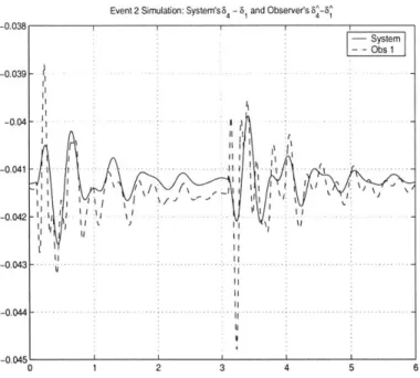
Simulation of Event 2: Results for Event 2 are shown in Figures 3-5, 3-6 and 3-7. Figure 3-5

shows the relative angle 631 at the generator bus nearest to the affected line, and its estimate

631. Notice that 631 reflects the correct general form of 631 during the event period, but a constant angle difference is evident, mostly due to the observer's lack of the information

Event 1 Simulation: System's 8 -8 and Observer's ^-5^ -System -- Obs1 I q - --- -. . - - - -- -.. t - - -I - - V - - - -- - - ----

~ ~ ~ ~

-. -.-- --... -. ...- - - -.. - ...- - - --. -. --. ...-. ..---...---- -. ...-. -- -- -.-- .-- 1 2 3 4 5 6

Figure 3-3: Time plots of 65-61 (system) and 13-SI (observer) when Event 1 occurred (be-ginning at t = 0.1s, duration 3s). 0.1 0.05 0 -0.05 -0.1 -0.15 -0.2 -0.25

Event 1 Simulation: System'su₃and Observer's

0 1 2 3 4 5 6

Figure 3-4: Time plots of w3 (system) and w3 (observer) when Event 1 occurred (beginning

at t = 0.1s, duration 3s). -0.073 -0.074 -0.075 -0.076 -0.077 -0.078 -0.079 -0.08 -0.081 -0.082 0 Syste -- Obs 1 IiIt : i I~

~

III. t It iIt I. I -i - -it -.-. -- -.- -.- - - .- . --. - - -. -. -. -. -. -. -. -. -.-.-. . .1. . . . .. . . .. 1 . . .. . .1 . .. --l - -- -i -t - - -- - - -- - -t - - - t i- - -

-uuua

-.1

Event 2 Simulation: System's ₃ -8 8 and Observers 8^_-A 0.105 System -- Obs 1 0.1 0.095 -0.09 - .-. -..- . -. . -0.085 - - -t- - *- --0 .0 8 - - - .... ..- . .. .- -.-.-.-.- .. .. . -. ...-0.075I- - t . - - - ...-.- -. 0.07

Figure 3-5: Time plots Of 63-JI (system) and 3-S1 (observer) when Event 2 occurred (be-ginning at t = 0.1s, duration 3s).

regarding the change in network topology. After the event the observer estimates J31 well, although some steady-state discrepancy persists due to model mismatch between the system and the observer. Similar explanations are also applicable to the 64, and J41 plot in Figure 3-6 and to the 6, and 661 plot in Figure 3-7. In Figure 3-7, the algebraic nature Of J6 is

evident in the instantaneous angle

jumps

3.2

Selecting the

Q

and R Matrices

The process noise and measurement noise intensity matrices,

Q

and R respectively, influence the observer gain matrix L through (2.18) and (2.19). If the process noise is significantly larger than the measurement noise, the observer will preferentially weight the measurement information relative to the dynamic model. On the other hand, if the measurement noise is significantly larger than the process noise, the observer will not trust the measurements and will essentially run in an open loop, i.e., as an uncorrected real-time simulator.

Even in the absence of process and measurement noise,

Q

and R may be used as design

isuch jumps _{are only possible for the algebraic variables, not for the differential variables such as the}

-0.038 -0.039 -0.041 -0.041 -0.042 -0.044 0

Event 2 Simulation: System's ₄ - 1 and Observer's 4 ^

-- System Obs I * It -.-.-.- - ---. ....-. ..-. ...-. -. ... .-. .- . -...... .... ... ... 1 2 3 4 5 6

Figure 3-6: Time plots of 64-61 (system) and 34-61 (observer) when Event 2 occurred (be-ginning at t = 0.1s, duration 3s).

Event 2 Simulation: System's86 - and Observers 6^-1

_.n net. -0.066 -0.068 -0.07 -0.072 -0.074 -0.076 -0.07f 0 1 2 3 4 5 6

Figure 3-7: Time plots of 66-61 (system) and 16-11 (observer) when Event 2 occurred (be-ginning at t = 0.1s, duration 3s). -System - Obs1 - I -t --... ... ... .. . -I - - - - -- - --- --t _{. . . .}-_{. ..} .. . . . . .. . . . . . .

parameters for the observer. Adjusting their relative values allows one to weight the observer towards heavy reliance on the measurements, or heavy reliance on the model, or a range of intermediate compromises.

For our investigations we chose

Q

and R to both be diagonal matrices. The results2 simulate as shown in this thesis are for the case in which each diagonal entry of

Q

is 25 x 10-8, while the diagonal entries of R are 64 x 10-10 in the positions corresponding to direct angle measurements, and 64 x 10-8 in the positions corresponding to the remaining three types of measurements. A more comprehensive examination of the effects of varying

Q

and R is needed, but left for future study.

3.3

Types of Measurement and Placement

The choice of sensor types and of their placement plays a key role in designing good ob-servers. However, comparing and rank-ordering different choices of sensors and placements is not straightforward, because several factors are involved.

If we commit to choosing the observer gains through the LQE methodology, and if

Q

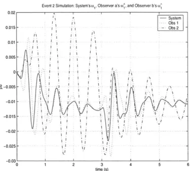
and R indeed represent the intensities of white process and measurement noises, then P in (2.18) represents the error covariance matrix of the state estimate. One could then use, for example, a weighted sum of the state component error variances - i.e., a weighted trace of P - as a measure3 _{of observer quality for each choice of sensor types and placement. A} more thorough study of this possibility is left to future work, but we present an illustration here.

The plots in Figure 3-8 show the results obtained under the same Event 2 scenario considered in Figures 3-5-3-7. Observer a is the observer used in all the results shown so far, while Observer b uses the same three types of sensors, but placed differently: a direct angle sensor at bus 9; a power injection sensor at bus 5; and a power flow sensor on the line directed from bus 4 to bus 5. The (unweighted) trace of P for Observer b (7 x 10-6) is one order of magnitude larger than that for Observer a (7.7 x 10-7), indicating that Observer b is poorer than Observer a. The waveforms compare the actual W, (full line) with

2

We achieved this results by adjusting the values of Q and R until we saw obvious but mild effects of the noises on the states of the system.

3

One difficulty we are experiencing here is a physical interpretation of this measure because the state vector has both angles and speeds as its components; therefore, the weighted sum actually combines both units.

Event 2 Simulation: System's ,, Observer a's o and Observer b's W^ 0.02 - System -- Obs I 0.015 - Obs 2 0 -01 0.005 -01 -CL-0.005 - - -. --0.01 - ---0.015 -~I -0 .02 - ... .. .. . . .. . . . . -0.025 ' 1 -0.03 0 1 2 3 4 5 6 time (s)

Figure 3-8: Time plots of 64-61 (plant), s o-61 (suboptimal) and 37 -61 (worst case compan-ion) when "event 1" occurred (beginning at t = 0.1s duration 3s).

the estimates W (dashed line) and W1 (dot-dash line) provided by the two observers. The differences in performance are clearly visible.

3.4

Pole Placement VS LQE

This section presents results from a simulation comparing the performance of the network observer with the LQE linear gain to the performance of the network observer with a gain computed using pole placement. Pole placement is another filter design technique [9] used in control. This technique provides an easy-to-understand but powerful way to control the steady-state convergence rate of the observer although the choice of desirable pole locations is not always clear.

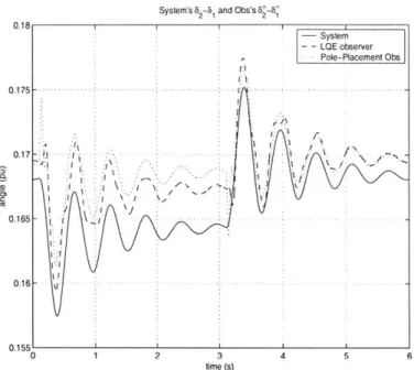
Figure 3-9, Figure 3-10 and Figure 3-11 present the state evolutions of the classical 9-bus system and two observers for Event 1. The first observer using the LQE technique is the same one we used in previous sections, but the other one is based on the pole placement technique and still uses the same three sensors that the first observer does. Note that the gain of the second observer is designed so that all the eigenvalues of (A - LC) are equal to

System's 82-5 and Obs's 6^-S^ 0.1 0.175 0.17 -a 0.165 0.16 0.155' 0 1 2 3 time (s) 4 5

Figure 3-9: Time plots of 62-61 (system) and 62-61 (for both LQE observer and pole-placement observer) when Event 1 occurred (beginning at t = 0.1s, duration 3s).

A's eigenvalues4 (in (2.14)) shifted by -1 and multiplied by 10 to give an observer that is

around 10 times faster than the system.

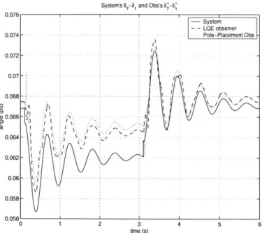
Figure 3-9, Figure 3-10 and Figure 3-11 show that our LQE observer outperforms the pole-placement observer in predicting the real state evolutions even during Event 1; how-ever, Figure 3-12 shows that the pole-placement observer and the LQE observer can also perform equally well. Although the results in this section suggest that our LQE observer usually performs better than the pole placement observer, there should be more comparative research on their performances. We leave this for future study.

4

A always has a zero eigevalue due to its structure

-System - -LQE observer - Pole-Placement Obs - - -. -. -.-.-.-.-.- -. _--. ...

-V

0

I I I I I

System's 87-81 and Obs's ^ 076 - System - LQE observer 074- Pole-Placement Obs 072 -- --- ---.07 - -068 - - - - - -066 - --064 - 062-.06 - - - 058-0 1 2 3 time (s) 4 5 6

Figure 3-10: Time plots of 67-61 placement observer) when Event 1

0.6 0.4 0.2 0.2 -0.4 -0.6 (system) and 67-61 occurred (beginning

System's w and Obs's ^

-System - - LQE observer - Pole-Placement Obs t- lt - -- --. - - - --- -- _t- t -. .. .- -.. -. . . . .. ... ...... ... ... ... . .. --0.8 1 1 2 3 time (s) 4 5 6

Figure 3-11: Time plots of w6 (system) and C26 (for both LQE observer and observer) when Event 1 occurred (beginning at t = 0.1s, duration 3s).

pole-placement 0. 0. 0. C1._0. 0. 0. 0.

(for both LQE observer and pole-at t = 0.1s, durpole-ation 3s).

0

System's 54- and Obs's 8^-5^

2 3

time (s)

4 5 6

2: Time plots of 64-61 observer) when Event

(system) I occurred

and 64-61 (for both LQE observer and pole-(beginning at t = 0.1s, duration 3s). - System S LQE obs - Pole-placement obs -5- q--~~. -. -. -. --- -. - -. .. . ... -. ..-. -. -. -. --. -. ..--. ... --. . - --- - ..-- ...-- - - --...-- - . .--. -.-.-.-.-. .-.-.-.-.-.-. .-.-.-.-.- -..- .-.-.- .- .- .- .-. -. --0.04 -0.0405 -0.041 -0.0415 a -0.042 -0.0425 -0.043 -0.0435 -0.044 -0 0 Figure 3-1 placement I44

Chapter 4

Fault Isolation Applications

The observer studies we did in the previous chapter showed that our nonlinear observer can give us satisfactory numerical results. This chapter provides two simple case studies showing that the nonlinear observer is also capable of achieving effective fault isolation. The first study concerning the multiple observer scheme is a simple fault isolation method that functions effectively with small networks. The other study instead uses a single nominal observer to achieve the task; however, the diagnosis process is possible only through un-derstanding the pattern of the steady-state output error (

y)

vectors. We then proceed to gain insights into the relation between the EY vector and line perturbations through Taylor series expansion analyses based on (2.2) and (2.5).

4.1

Multiple Observers for Fault Isolation

Fault isolation can be achieved via many ways; however, here we implement a simple but accurate and robust method of multiple observers

[3].

The main idea is to have several observers work concurrently in real time. Since our focus in this study is only on a complete single line-out fault, the model assignments to the observers are such that one observer has the nominal model of the system, and each of the rest has the nominal model with one unique line taken out. With such a set up, ideally one would expect that the observer whose model matches the current model of the real system will outperform the other observers in terms of predictions at the steady-state.

The scheme prompts us to further investigate via simulations its applicability in fault isolation of power systems. Therefore, we put the method of multiple observers into tests

on the classical 9-bus system.

Multiple Observers in Simulation Tests: Here, we examine the performance of the

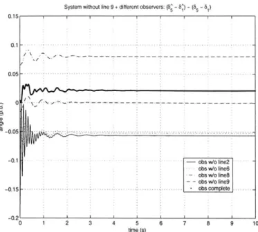
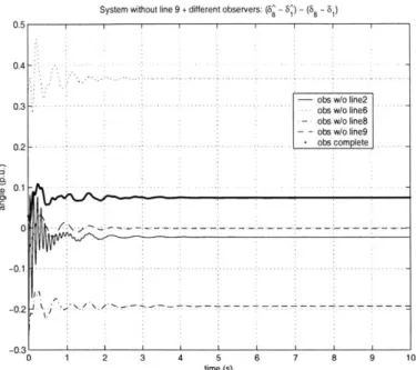
multiple-observer scheme via simulations on the classical 9-bus system. In these simulations, the real system with the nominal model has Line 9 for the line numbering of the classical nine-bus network. taken out at the start1 , and there are ten different observers running independently and concurrently. Note that although having different models, each observer consists of the same three sensors that we used before in the previous chapter. Also, both the real system and the observers start off with the same initial condition, which is the loadflow solution of the nominal system. Therefore, we can see the transients of the real system and all the observers right after the simulations start.

From the above setup, one would expect that the observer whose model is nominal but without Line 9 will best predict the real states because its inherited model matches that of the real system. Our simulation results substantiate the claim. Figure 4-1, Figure 4-2 and Figure 4-3 clearly show that the model-matching observer outperforms other observers since its residual always converges to zero at the steady state, but those of the others do not.

Despite the simplicity and the accuracy of the multiple observer scheme, the approach is computationally intensive and unscalable for bigger and more complex systems. For example, in order to deploy the scheme to isolate a single-line fault of a power network, we need to have n

+

1 different observers for n lines. The linear growth of the computational burden with the number of lines in the network poses a serious problem in real-time state estimations.

Although constrained by its requirement for large computational power, the multiple observer scheme does not only have a virtue of being a good method for fault isolation of small networks, but also illuminates the significance of the model inherited in the fault detection observer to achieve the optimal state predictions. In other words, failing to have the right model, the predictions of an observer will never be able to converge to the correct steady states and will either fall short by a constant offset at the steady-state because of the model discrepancies between its model and that of the real sytem, or will diverge away from the steady state.

Ideally, one would want to have an economical and efficient algorithm for the fault

System without line 9 + different observers: (8^ -8^) -(8 -8)

----

--- - -- - ---- ---- -- --- - - -

-- - - - --- - -

-- --- - - - -- - -- -- -- - obs w/oline2 -obs w/o line6

---obs w/o lineB

-obs w/o line9

-. -.-..-..- scomplete

-0.2'

0 1 2 3 4 5

time (s)

6 7 8 9 10

Figure 4-1: Time plots of the residuals (05-61) - (65-61) of different observers when the real

system has Line 9 taken out.

0.15 r

0

0.05

System without line 9 + different observers: (8^- 8) -(8 _ ) obs w/o line6 obs w/o line8

- -obs w/o line9 .1 - -.- - - - obs complete -0 -0.05 -0.1 -0.151-.- --0. .. . . . .. . . . ... . .. . . . . . - - - - -- - --- ----1 2 3 4 5 6 7 8 9 10 time (s)

Figure 4-2: Time plots of the residuals (66-61) - (66-61) of different observers when the real

system has Line 9 taken out.

0.15 0.1 0.05 A? -0.05 -0.1 -0.15

2

0 co c Cd

(

System without line 9 + different observers: (6^ - ^ ( -8

0.5 1

0.4

- obs w/o line2

03.. obs w/o line6

- obs w/o line8

obs w/o line9

0.2 - . - -- - - - - -- -- .- - - -- - obs complete 0 .1. - - - - -- - - -- - -0- --0 .1 -. ..-. -.- --. . ... .- -- --.- -. .. .--.. -.. .. .-.. -.- -.-- . -.. . .-.-.- - -.- .- --- . aa -0.2 - ~~ ~ ~ ~ ~ - ~ --0.3, 0 1 2 3 4 5 6 7 8 9 110 time (s)

Figure 4-3: Time plots of the residuals (68-61) - (68-61) of different observers when the real

system has Line 9 taken out.

isolation of power networks. However, to achieve such a scheme, we had better well com-prehend the properties of the faults of interest. Having a solid understanding of the fault characteristics, we hope to use those properties as our fault identification criteria.

4.2

Understanding Faults on the Network: Line Parameter

Disturbances

This section investigates the effects of line-parameter disturbances on the classical 9-bus power network. The motivation is to shed light on interesting characteristics originating from line parameter disturbances in the hope that these observations will suggest useful insights for fault isolation application.

First we need to know what information we can use as inputs for our investigation. It is worth emphasizing that in practice the output of the actual system, the output of the observer (or the output prediction of the observer) and the predicted state evolutions are all the information we know. Therefore it is reasonable and obligated for us to focus on using this information to form a comprehensive framework for understanding faults in the real system.

However, before getting deeper into details about faults, we need to know about the normal operation of the system, so that we have a basis for comparisons in future studies about faults.

4.2.1 Normal Operation

In order to understand faults well, we need to realize what happens at the normal operating point. Such knowledge can be helpful when we want to have a base for comparison and for suggestions about the behavior of the network after a fault occurs. Here we show the steady-state angle values of all the nodes and the steady-state loadflow values for all the lines in the classical 9-bus example in Figure 4-4, under the operating conditions labeled in the figure. Note that the direction of the arrow on each transmission line indicates the power flow direction.

Note that we are assuming that all transmission lines of the network are lossless. As a result, the power injected into one end of a line equals the power coming out at the other end of the line. Another interesting consequence is that the power injections of all generators (e.g., node 1, node 2 and node 3) into the network equal the power extractions of load buses (e.g., node 5, node 6 and node 8) from the network. Also, from our observation, the absolute angles of all the nodes always keep decreasing right after the simulation starts2, but the absolute speeds of the generators will first slightly fluctuate downwards and eventually reach steady-state values.

4.2.2 Investigation of the Steady-State Output Error Vectors

The seminal thesis of Beard [10] ;suggests that each fault will affect the network behavior to generate a certain geometric pattern of the corresponding steady-state output error 3 vector

(iy) used in the observer; therefore, we begin our study by doing simulations to scrutinize the pattern.

2

This phenomenon will not be problematic to us because we are interested only the evolutions of relative

angles. The reason is that, by looking at (2.2), we can see only relative angles, not the absoluate angles, play a role in determining to values of f(x, u, w).

3

Sno"m = -0.0427put Line 2 1.6307 p.u.

nom

2 .1149pu

94

2

PO" = -0.1313pu Line 8 0.7627 p.u.

4

Line 9 0.2430 p.u.

8

Line 6 0.8680 p.u.

5

6

Line 4 0.4083 p.u. 4P' = -0.0962pu 0.7173 p.u. Line 1 nom = -0.0179pu

9

Line 3 0.8505 p.u.

3

63"' = 0.032pu Line 7 0.6075 p.u. P"' = -0.1255pu Line 5 0.309 p.u. no " = -0.0548pu

Figure 4-4: Normal operation of the classical 9-bus sytem: angles and power flows.

'7

7 o, = 0.0128pu