Decorrelation time of speckle targets observed with a heterodyne-reception optical radar

WITH A

HETERODYNE-RECEPTION OPTICAL RADAR by

SUN TONG LAU

B.S.E.E., State University of New York at Buffalo (1980)

SUBMITTED IN PARTIAL FULFILLMENT OF THE REQUIREMENTS FOR THE

MASTER OF SCIENCE at the

MASSACHUSETTS INSTITUTE OF TECHNOLOGY June 1982

Signature of Author...

Department of Electrical

Certified by...

... Engineering and Computer Science

June 30, 1982

//e'ffrey

1.

V

Accepted b .

Arthur C. Sm th Chairman, Departmental Committee on Theses

Archives

OF TECHNOLOGY

OCT 20 1982

DECORRELATION TIME OF SPECKLE TARGETS OBSERVED WITH A

HETERODYNE-RECEPTION OPTICAL RADAR

by

SUN TONG LAU

Submitted to the Department of Electrical Engineering & Computer Science on June 30, 1980 in partial fulfillment of the requirements for the

Degree of Master of Science.

ABSTRACT

Coherent laser radars provide new technology for a variety of target detection and imaging scenarios. However, poor-image quality is caused by laser speckle resulting from the shortness of the laser wavelength compared to the surface roughness of typical targets. Serious signal return

fluctuations are found whose time dependence is poorly understood. The purpose of this thesis is to assess the time dependence of speckle target radar returns. A data processing technique is developed to investigate the correlation property of the laser radar data. Accordingly, useful insights concerned with the causes of the return fluctuations are obtained. A

mathematical model, which incorporates random radar and target tilts, is then constructed to describe the decorrelation process of the radar returns. Comparison of experimental results and theoretical results shows that

atmospheric turbulence and wind are the factors which control the decorrela-tion process.

Thesis Supervisor: Jeffrey H. Shapiro

ACKNOWLEDGMENTS

I would like to thank my graduate counselor and thesis advisor Professor J. H. Shapiro for his patient guidance and invaluable advice during my studies at M.I.T. and the course of my thesis research. It has been my pleasure to work with him and learn so much from him.

I also wish to acknowledge all members of the Optical Propagation and Communication research group at M.I.T. especially Dr. D. M. Papurt and T. T. Nguyen. Valuable suggestions from them have added to this work.

Thanks are also due to members of the Opto-Radar Systems group at M.I.T. Lincoln Laboratory. R. J. Hull, T. M. Quist and R. J. Keyes should be mentioned for their help in providing me with the radar data and computer facilities for this research.

Financial support by the U.S. Army Research Office, Contract DAAG29-80-K-0022 is gratefully appreciated.

Elain Aufiero, Donna Gale and Deborah Lauricella deserve mention for their excellent typing.

To my mo.ZheL,

TABLE OF CONTENTS Page ABSTRACT... 2 ACKNOWLEDGEMENTS... 3 TABLE OF CONTENTS... 5 LIST OF FIGURES... 7 LIST OF TABLES... 9 CHAPTER I. INTRODUCTION... 10

I.l. Laser Radar Configuration... 10

1.2. Intensity Fluctuation of Speckle Targets-Problem Statement... 11

1.3. Thesis Overview... 16

Chapter II. STATISTICAL PROPERTIES OF THE INTENSITY FLUCTUATIONS... 18

II.l. Scintillation-sensor/Radar Data Description... 18

II.1.1 Atmospheric Turbulence... 18

11.1.2 Scintillation Measurements... 19

11.1.3 Staring-Mode IRAR Data... 21

11.2. Correlation Coefficient Function (CCF) Estimation... 21

11.2.1 CCF Estimation Procedure... 22

11.2.2 CCFs in Various Turbulence Levels... 24

CHAPTER III.

CHAPTER IV. REFERENCES....

MATHEMATICAL MODELING... III.1 Theoretical Model... III.1.1 Model Derivation. 111.1.2 Model Interpretat 111.2 Model Verification... DISCUSSION... ... o... on Page 44 44 45 54 67 84 87

LIST OF FIGURES

Radar Block Diagram... Formation of a Speckle Pattern... Autocorrelation Function of the Gate Function, g(t)... Estimated Autocovariance Function of x(t)... Estimated Correlation Coefficient Function of y(t)... CCF of Data Set 1... Set 2... Set 3... Set 4... Set 5... Set 6... Target-Return of Data Set 1. Target-Return of Data Set 2. Target-Return ... Intensities vs. Intensities vs. ... . Intensities vs. ... Intensities vs. ... Intensities vs. ... Intensities vs. ... Expected Expected Expected ... Expected ... Expected Expected ... 7 CCF of Data 8 CCF of Data 9 CCF of Data 10 CCF of Data 11 CCF of Data 12 Histogram of Frequencies 13 Histogram of Frequencies 14 Histogram of

Frequencies of Data Set 3. 15 Histogram of Target-Return

Frequencies of Data Set 4.. 16 Histogram of Target-Return

Frequencies of Data Set 5.. 17 Histogram of Target-Return

Frequencies of Data Set 6.. Radar Configuration... Figure

1 2

Theoretical CCFs with Only Radar Tilt Active... Page 12 14 25 26 27 28 29 30 31 32 33 38 39 40 41 42 43 46 3 4 5 6 18 19 ... .. I. .. . .. .. .. .. ... .. . .. . .. ... . . . . . 57

Theoretical CCFs with Only Target Tilt Active... 21 Theoretical Active,R > 1 22 Theoretical Active,R > 1 23 Theoretical Active, R > 24 Theoretical Active, R < 25 Theoretical Active, R < 26 Theoretical Active, R < 27 Theoretical 28 Theoretical 29 Theoretical 30 Theoretical 31 Theoretical 32 Theoretical 33 Best CCF Fit 34 Best CCF Fit 35 Best CCF Fit 36 Best CCF Fit 37 Best CCF Fit 38 Best CCF Fit CCFs with both and a; > G .. CCFs with both and a0 = a . CCFs with both l and au < a. CCFs with both 1 and a < a CCFs with both 1 and a; = a . CCFs with both 1 and a; > a'.

Radar and Target Tilts ... ...

Radar and Target Tilts

... Radar and Target Tilts

... Radar and ... Radar and ... Radar and CCF vs. Experimental CCF CCF CCF CCF CCF of of of of of of vs. Experimental vs. Experimental vs. Experimental vs. Experimental vs. Experimental Data Set 1... Data Set 2... Data Set 3... Data Set 4... Data Set 5... Data Set 6... CCF CCF CCF CCF CCF CCF Target Tilts ...T e... Target Tilts ... o... Target Tilts of of of of of of Data Data Data Data Data Data Set Set Set Set Set Set 1. 2. 3. 4. 5. 6. Figure 20 Page 58 60 61 62 64 65 66 71 72 73 74 75 76 77 78 79 80 81 82

LIST OF TABLES Table

1. Scintillation Measurement Results...

2. Decorrelation Data...

3. Parameters for Figures 21, 22,

4. Parameters for Figures 24, 25,

5. Estimated a e and

-23 ...

26 ...

from Turbulence Theory...

6. Parameter Values for Best CCF Fit... Page 20 34 63 67 69 83

CHAPTER I

INTRODUCTION

Heterodyne-reception optical radars using the 10.6 -rm wavelength CO₂ laser provide new technical options for a variety of target detection and imaging scenarios [1]. However, the much shorter wavelength of laser radars as compared to microwave radars implies new problems as well as enhanced capabilities [2]. One of the problems is the poor image quality which is caused by laser speckle [3], resulting from the shortness of the laser wave-length compared to the surface roughness of typical targets. Serious signal return fluctuations are found whose time dependence is poorly understood. This research will be addressed to assessing the time dependence of speckle target radar data analysis and theoretical modeling. The remainder of the introduction includes a description of the optical radar we are using, a problem statement, and an overview of the thesis organization.

I.1: Laser Radar Configuration

An ongoing program aimed at developing an Infrared Airborne Radar (IRAR) is underway at the M.I.T. Lincoln Laboratory [4] [5]. A radar testbed system has been constructed as part of this program which we will refer to as IRAR, although it is ground mounted. Data for this thesis has been obtained using IRAR. This laser radar uses a one-dimensional, twelve-element HqCdTe hetero-dyne detector array, a transmit/receive telescope of 13 cm aperture, and a 10 W CO2, 10.6 um laser, which is operated in pulsed mode. Presently, we are

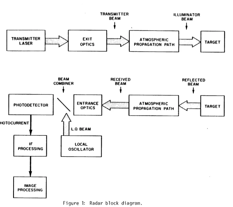
kilometers. More radar system descriptions can be obtained in [2] [4] [5]. In order to set up subsequent statistical system analysis, the basic structure of a heterodyne-reception optical radar is explained. It can be represented by the block diagram of Figure 1 [5]. The laser radar sends out a series of pulses and illuminates a target located a certain distance away. After passing through the exit optics in Figure 1, the laser beam propagates

through the atmosphere and the illuminator beam is reflected back by the target. The reflected beam then comes back through the atmosphere and the entrance

optics. Finally, the received beam is combined with the strong local oscillator beam operating at a frequency offset v IF on the surface of the photodetector. In target-detection applications, the IF signal is to be used to estimate the average target reflection strength which is compared with a threshold value to determine the presence or absence of a target. In performinq imaging, the radar first scans the target and collects arrays of echo signal returns in order to form a complete picture. Then, computer enhancement of the resulting

image follows, after the estimation of the average target reflection strength is finished.

1.2: Intensity Fluctuation of Speckle Targets - Problem Statement

The random intensity distribution that we call a speckle pattern is formed when fairly coherent light is either reflected from a rough surface or propagates through a medium with random refractive index fluctuations [3]. Since the wavelength of the CO2 laser is 10.6 -pm, many target surfaces are

rough on the order of a wavelength. As a result, the surfaces scatter the light diffusely and form a speckle pattern. The observation at a distant point

TRANSMITTER EXIT ATMOSPHERIC

LASER OPTICS PROPAGATION PATH TARGET

BEAM

COMBINER RECEIVEDBEAM REFLECTEDBEAM

EN T RANCE A TMOSPHE RIC

OP TICS PROPAGA TION PA T H T G

L.O. BEA M LOCAL OSCIL LA TOR PHOTODETECTOR PHOTOCURRENT IF PROCESSING IMAGE PROCESSING

scatterers as in Figure 2. Obviously, if the point of observation or the precise position of the target being illuminated is changed, the signal return intensity will change at the same time. Statistically, the speckle fluctuation obeys an exponential probability distribution

p(I) = exp

[-

where I = signal returns intensity <I> = ensemble average intensity.

It can be seen that speckle in infrared radar is an analogy to the Rayleigh cross-section fluctuations in a conventional radar. Intensity fluc-tuations of the magnitude associated with the exponential distribution create

serious problems in imaging. However, averaging several independent image frames will result in significantly better overall image quality. The question then becomes one of obtaining independent image frames, i.e., of determining the decorrelation time for the speckle process.

The exponential distribution cited above rigorously applies to the target-return intensity flucutations over an ensemble of macroscopically

identical rough-surface targets. The exponential distribution has been verified experimentally by Papurt [7] via spatial sampling of the speckle fluctuations in IRAR images obtained form a large rough-surface target of uniform average reflectivity. In this spatial sampling, the target returns from non-overlapping illumination regions on the surface are independent samples from the expon-ential distribution. Because the use of spatial averaging to reduce speckle fluctuations in a laser radar image will necessarily entail a loss in spatial

Figure 2: Formation of a speckle pattern.

SURFACE

resolution, it is important to study the time averaging of intensity returns reflected from a single spot of the speckle target. To probe the time-averaging issue the radar can be operated in staring mode, that is with its scanning

capability disabled. If the target, the radar,and the intervening propagation medium are perfectly rigid, then the radar will stare at one spot on the

target and there will be no time dependence to the intensity returns. Prelimin-ary staring mode IRAR measurements have shown, however, serious fluctuations of the intensity returns in time. It is important to know the time correlation properties of these fluctuations since they will impact radar performance, e.g., the use of frame averaging to reduce speckle fluctuations in the radar image requires inter-frame time separations that are longer than a coherence time. Also, the contributing factors for the staring-mode fluctuations are not known yet. It is significant to see how these factors affect the decorrelation process as it may help guide future improvements in the radar system. The major objectives of this thesis are two fold. First, to investigate the time correlation properties of staring-mode speckle target intensity fluctuations. Second, to explore the causes of the decorrelation mechanism.

For the simple geometry in Figure 2, the causes of the decorrelation process are probably the atmospheric turbulence effects along the laser prop-agation path, and the wind induced vibrations of the IRAR equipment and the target. Staring-mode IRAR data will be used to study the decorrelation process. Simultaneous scintillation-sensor measurements will be used to estimate

atmospheric turbulence levels. Thus, we shall be able to compare the time correlation properties of radar data taken in various turbulence strengths.

To properly account for the speckle target intensity return fluctuations, the probability density function and the correlation coefficient function in

time should be known. The former furnishes information concerning the properties of the intensity fluctuations in the amplitude domain, whereas the latter describes the degree of correlation of the data in the time domain. In the latter case, we will determine the decorrelation time, i.e., the time it takes for the data to become uncorrelated, from IRAR measurements. Using this decorrelation time, a collection of uncorrelated

samples will be extracted from the IRAR data and compared with the exponential ensemble statistics predicted for the former case.

In support of the data examination, a mathematical model is developed to describe the decorrelation process. This model assumes free

space propagation with random radar aiming errors and random target tilts. These statistical quantities may represent turbulence-induced phase

tilts whose strengths can be estimated from turbulence theory using the scintillation measurements. With these estimated values the

predictions of the decorrelation model will be compared with experimental results from the radar data.

1.3: Thesis Overview

In Chapter 2, we begin with a complete description of the radar data format. Then the procedure for estimating the correlation coefficient function is explained. Correlation results based on IRAR data taken in various atmospheric turbulence levels are presented. Finally, a chi-squared goodness-of-fit test for the exponential distribution is performed on

some insight into the nature of the intensity fluctuations.

In Chapter 3, our model for the decorrelation process is postulated and analyzed. We shall exhibit the behavior of the model as its parameters are varied. The correlation coefficient predictions of the theoretical model are then compared with the experimental radar results of Chapter 2. Chapter 4 contains a discussion of the target

return time dependence as understood from our experimental and theoretical results.

CHAPTER II

STATISTICAL PROPERTIES OF THE INTENSITY FLUCTUATIONS

This chapter is devoted to our experimental efforts aimed at under-standing the decorrelation process. We begin with a brief discussion of atmospheric turbulence and a summary of the scintillation sensor data. The format of staring-mode IRAR data is then described. Next, we shall explain the detailed procedure for estimating the correlation coefficient function

(CCF) of the IRAR data. Subsequently, CCFs for six data sets taken in various turbulence levels are presented. Finally, chi-squared goodness-of-fit tests to the exponential distribution are performed on the six data sets.

II.1: Scintillation-Sensor/Radar Data Description

Radar data taken from the IRAR has been investigated in order to

understand its basic statistical properties. It was taken in various turbulence levels with scintillation measurements made simultaneously. Theory for wave propagation in the turbulent atmosphere has been well established during the past decade [8] [9]. In order to provide pertinent information relevant to our research, turbulence effects on laser propagation in atmosphere is intro-duced first. Second, we shall explain the scintillation measurement and its implications. Then, the radar data description is given at the end of this section.

II.1.1: Atmospheric Turbulence

which are due to turbulent mixing of air parcels of nonuniform temperatures in clear weather conditions. These air blobs will dephase an optical wave, hence causing transmitter beam divergence and receiver angle-of-arrival fluctuations. Also, the random lensing of the wave by the turbulence leads to constructive and destructive interference, i.e., amplitude fluctuations, called scintillation.

These effects on laser propagation were described for a time independent medium. In the atmosphere, since the array of turbulent eddies tend to drift with the nominal wind velocity. Consequently, the turbulence has a typical

coherence time tc of 10-3 to 10-2 seconds [101. We strongly suspect that turbulence effects are the prime factor controlling decorrelation time in staring-mode speckle-target measurements. As we go along, the intuition from the data manipulation and the statistical modelling should help justify this statement.

11.1.2: Scintillation Measurements

The turbulence strength along the atmospheric path between IRAR and

the speckle at a particular time can be estimated from the amplitude fluctuations (scintillation) of laser pulses that have propagated over this path. To

perform this scintillation measurement, two lasers, CO2 and GaAs, were located

next to IRAR with their receivers located one kilometer away adjacent to the speckle target. Data acquisition equipment and data processing programs have been developed at Lincoln Laboratory to produce good estimates of the turbulence strength parameter, Cn2 [5] and the atmospheric coherence time tc from the

received CO2 and GaAs laser pulse streams. Six sets of scintillation data were

C and t are summarized in Table 1, where they have been ordered

n c

according to their turbulence strength.

TABLE 1

Scintillation Measurement Results

Data Set Number 1 2 3 4 5 6 Cn2 _m-2/3) 0.95 x 10l 4 0.87 x 10-13 0.107 x 10-12 0.13 x 10-12 0.2 x 10-12 0.34 x 10-12 tc (ms) 39 23 45 16 26 52

11.1.3: Staring-mode IRAR Data

The IRAR data was taken in staring mode using the Lincoln Laboratory flame-sprayed aluminum speckle-target calibration plate at one kilometer range. The pulse-repetition frequency of the radar is 18.9 KHz, correspond-ing to an inter-pulse time interval of approximately 52 vi sec. Even in staring mode IRAR data is recorded in frames of pictures. Each frame has 128 by 60 picture elements (pixels) which are linearly proportional to the return strengths of the associated laser pulses. Unfortunately, the data is not taken in a completely continuous manner, thus giving rise to some difficulty in computing the statistical properties such as the CCF. The details were as follows. Each frame has 60 active lines of 128 data points each plus 82 missing data points because of hardware mechanics. Because of the periodic missing information, we had to formulate a procedure to

estimate the CCF from such an intermittent structure. Discussion of the CCF estimation procedure forms the essence of this chapter. It should be noted that the data which we deal with is the square of the IF signal envelope, because the squared envelope is proportional to the return light intensity. 11.2: Correlation Coefficient Function Estimation

The CCF for a wide-sense stationary random process y(t) with auto-covariance function Kyy(v) is

CCF(v) = Kyy(v) / Kyy (o)

It is well known that CCF(v)I < 1 with ICCF(v)| = 1 when y(t) and y(t + v) are completely correlated, and CCF(v) = o when y(t) and y(t + v) are

uncorrelated. The decorrelation (or coherence) time of the process y(t) can therefore be defined as the time it takes for CCF(v) to drop from one to zero.

11.2.1: CCF Estimation Procedure

If the data were continuously spaced, a direct method could be

employed to compute the correlation coefficient function (CCF). Unfortunately, because of the regularly missing observations in the radar data, a special formulation had to be developed.

Let y(t), t = integer, be the discrete time stationary process

representing the data that would be gotten were there is no regularly missing observations. Let g(t) be the periodic gate function with period a + 3

g(t)

0

where a = 128 and B = 82.

If x(t) denotes the actual data,

t = a + 1 + +

we can write

x(t) = g(t) y (t)

We are interested in the CCF of the random process y(t), which is

CCF(v) = Kyy(v) / Kyy(o)

where Kyy(v) is the autocovariance function of the process y(t) and the latter is assumed to be wide-sense stationary. We shall use as our estimate

of CCF(v) the function

CCF(v) = Kyy(v ; T ; N) / Kyy (0 ; T ; N)

where Kyy (v ; T ; N) is a covariance function estimate based N data streams of length T obtained as described below.

Consider the following estimation equation,

A =1 T-vV

aV--Kxx(v ; t) = vF x(t) - my(Ti)g(t) 'x(t+v) - my(T)g(t+v) t=l

L

where Kxx(v ; T) = estimated autocovariance function of x(t) at lag v based on a T-length data stream,

T T

and m (T) = E x(t) / E g(t)

t=1 t=l

is the sample mean of all the non-zero data points. It is well known that my(T) is an unbiased consistent estimator of m the mean of the process

yy

y(t) [11]. Thus, if T is large we can use m (T) ~ m in Kxx(v T). It is then easily shown that

T-v

E[K xx (v ; T)] E _T~~~yt 1 y(t) - m )g(t)g(t Y + ++v-my]jv)[y(t + V) - m

T-V

T = g(t)g(t + v) E y(t) - my (y(t + v) - m

= R (v)K (v),

T-v

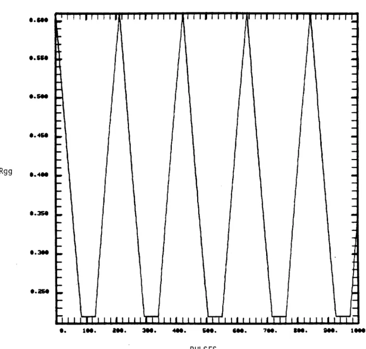
where Rgg(v)

Z

g(t). It can be shown that Rgg(v) is given by [61

,9 for v=o, ...

for v=, ... ,

,- for v=a, _{.. ,a6}

which is Dlotted in Figure 3.

It follows from the above that Kxx(v;T) / Rqg(v) is an approximately unbiased estimater for Kyy(v) for any T-length data stream that is long enough to ensure my(T) ~ my. The stability of this estimator depends on the

stability of Kxx(v;T), which will be good for v<<T and poor forvZ~T [12]. Improved stability can be obtained by taking Kyy (v;T;N) to be the sample mean of N Kxx (v;T) / Rgg(v) estimators obtained from N different T-length data streams.

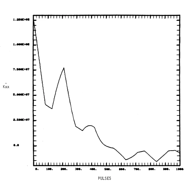
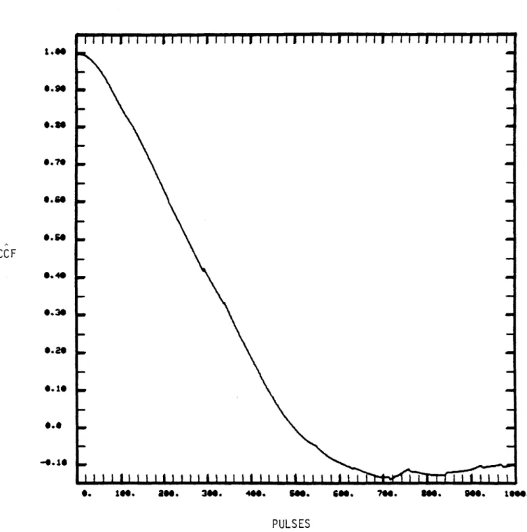
Our CCF estimation algorithm generates my(T) and Kxx(v;T) / Rgg(v) for N = 10 pictures each with T = 128x60 pixels. These were averaged

together to yield Kyy (v;T;N) and CCF(v) = Kyy (v;T;N) / Kyy(O;T;N). For the lag values of interest it was found that averaging the 10 pictures together gave satisfactory stability. Typical examples of Kxx (v;T) and CCF(v) are given in Figures 4 and 5, respectively.

11.2.2: CCFs in Various Turbulence Levels

0. 60 Rgg ,. 0.360 S. 3" 0.150 0. 1*. 0*. 3". 400. s*. 6*. 7". a". 9*. 10*. PULSES

II I III lI t I i i I lillIll Ii tII lilii II 5111191 I I 7.5 E+7 Kxx 5.ees*O7

a.seE+r7

II 1191111111111111111 IIlI 1111111 I||i 11111 Illill I

S. Ie. ae. 30. 4"0. 55. a"0. 750. 350. 950. 1SM.

PULSES

[[ii Iii ii i 511i 11 5 11i11 II ilil i ll Iii I i i ii 1111511 III I.00 0.90e CCF 0.40 0.30 *.ao 0.10 0.e 4.10 0. 100. a**. 300. 400. 500. 600. 700. 900. N00. 1000. PULSES

CCF

0.O5.

I I I I I I I I I I I I I I I I I I I I i i I I t.

. see. 1"s. Is"*. aese. 2500. 30*.

PULSES

-- -- r I i I I I I i i I i T

0.75

CEF

0.S

6. See. 1290. 10. 2OO. 25e0. 3000.

PULSES

~ I~~T ~ I I I T ~ ~ I I ' I I I I I I T o .50 .. CCF * .as 0.*5. I I I I I I I I I I I I I I I I

.Se. i*. ise.. as s25*. 3000.

PULSES

a.-IS

e.so

.

0.S

L . L I I. I I I I I I I I I I I

S. see. iee. isee. ee20. asee. 3900.

PULSES

0.75.-CCF .

as

S.ao0. IS". 50. 2000. a50e. 30".

PULSES

1.00

0.7S

O.Se

.l11. L1.I LL IIII 1 111 11111 I 111

lose. ise. ass.

5".

PULSES

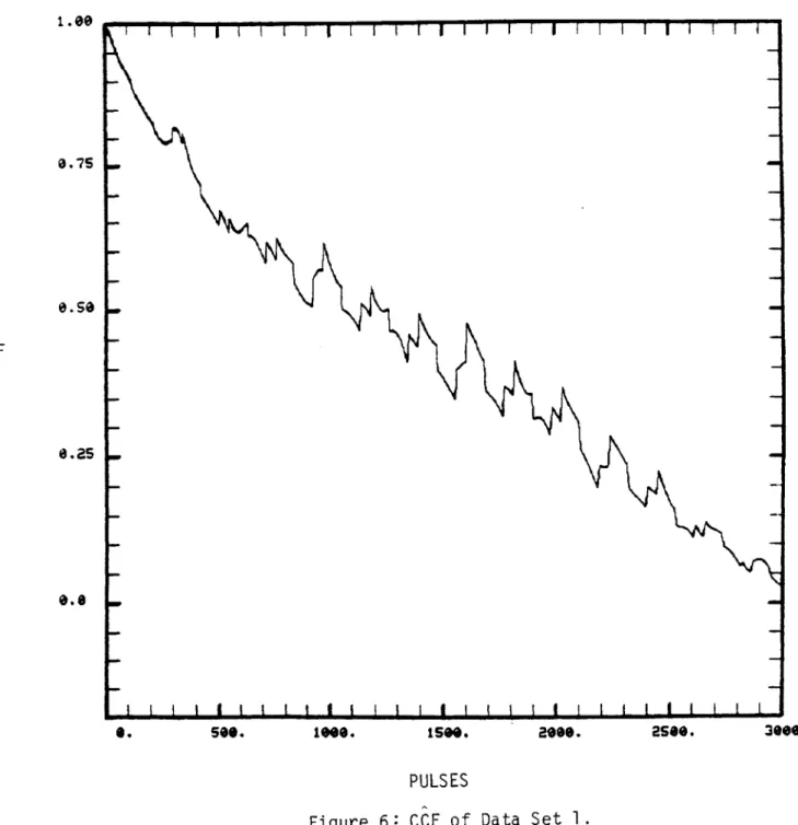
Figure 11 : CCF of Data Set 6.

..... CCF *.25 0.9 3000. -0.

For each figure we have computed the decorrelation time using the 52 vsec pulse spacing. The results are given in Table 2 along with the Cn2 values from Table 1, and the weather description recorded by the IRAR operators.

TABLE 2

Decorrelation Data

Data set no. Decorrelation Time (ms) _{Cn2 -2/3)}

0.95 x 10-~14 0.087 x 10-12 0.107 x 10-12 0.13 x 10-12 0.2 x 10-12 0.34 x 10-12 Haze, Overcast Hiqh Solid Cloud_Cover Partly Sunny Clear, Sunny Clear, Sunny Clear, Sunny

Two interesting points we can easily observe are:

1) Data Set 1 was taken in the weakest turbulence conditions, i.e., haze and overcast. It took 156 ms for the CCF to drop from one to zero which

implied that the data were highly correlated. In other words, the intensity return did not fluctuate very much in this data set.

2) The remaining data was taken in more or less the

Weather 1 2 3 4 5 6 156 65 78 39 39 52

same turbulence level, since the Cn2 values differed only slightly. On the other hand, the decorrelation times for Data Sets 2-6 varied from 39 to 78 ms.

An immediate implication of the first observation is that the intensity return fluctuations depend upon the atmospheric turbulence strength very much. In weak turbulence, the atmosphere is just like a "frozen" medium.

Therefore, the intensity returns stay constant for relatively long time periods. Conversely, the intensity returns start to fluctuate more as the turbulence strength gets stronger. The second observation leads us to suspect the other contributing factor, which is wind speed. As we shall see in the next chapter, wind speed in fact has an effect on the intensity return fluctuations.

11.3: Chi-squared goodness-of-fit test

The ensemble and spatial-sampling statistics of speckle-target radar returns obey the exponential distribution. In this section we shall use our six data sets to examine whether exponential statistics apply to staring-mode target returns from a speckle target. To make a quantitative assessment we will use a special type of hypothesis test called the chi-squared goodness-of-fit test, which is widely employed to test the equivalence of a probability density function of sampled data to some theoretical density function.

Since the decorrelation time for each set of data is known from the previous section, independent samples can be obtained. We first provide a brief description of the test and then give the test result in the sequel.

Consider N independent observations from a random variable x whose probability density function is p(x). Let the N observations be divided into K intervals to form a frequency histogram, where f. denotes the observed frequency in the ith interval. The number of observations which could be expected to fall within the ith interval if the true probability density function of x were p₀(x) is called the expected frequency, F .

To measure the discrepancy for all intervals, a chi-squared value is computed via

2 K' (f. - F.)2

X = F.

where K' is the number of intervals in which the expected frequency is higher than or equal to five. In other words, intervals in which F. is smaller than five are combined to form one interval. The number of degrees of freedom n is equal to K' - r - 1 where r is the number of parameters estimated from the data for the hypothesized distribution. Having obtained x2 and n standard statistical tables will provide a corresponding level of significance a which indicates how good the fit is. Generally a value of at greater than or equal to 0.05 is regarded as verifying the theoretical distribution. Further details about the test can be found in [12].

For our case we use the exponential distribution -1 -x/x x > 0

p (x) =

0 otherwise

where the mean x is set equal to the sample mean of the data. A sample of N = 210 independent observations was used for each of the six data sets.

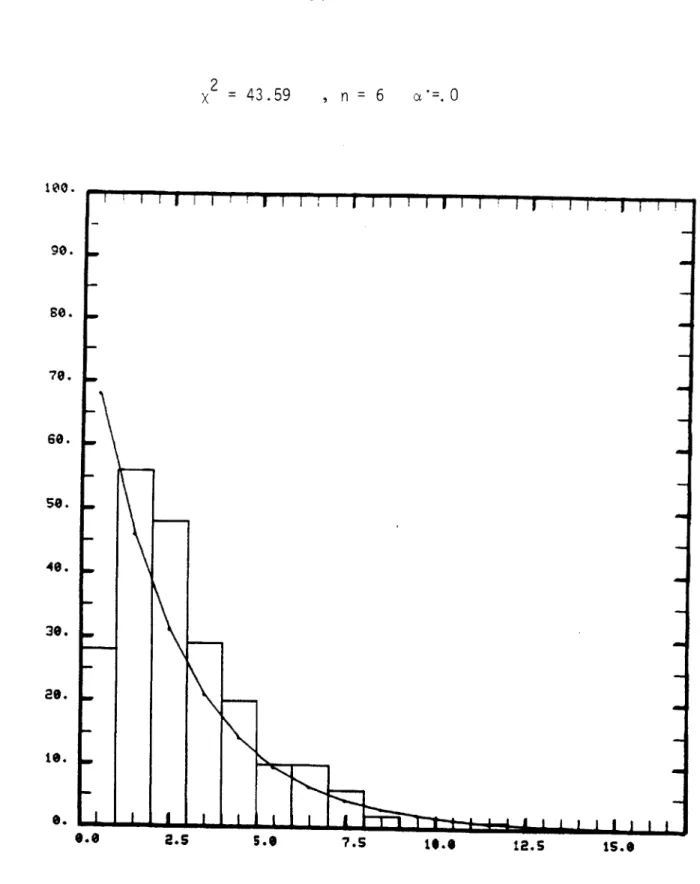
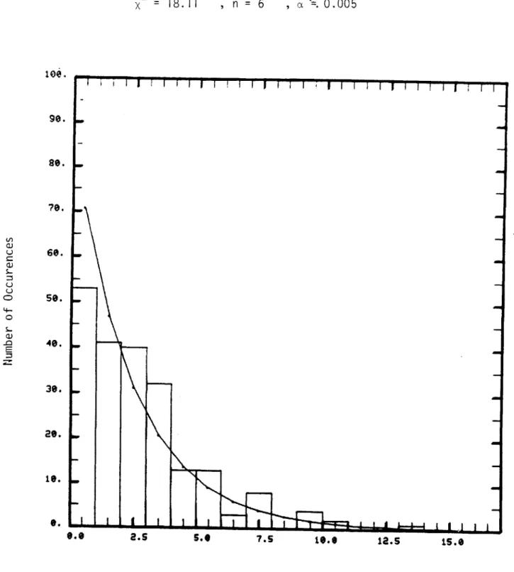
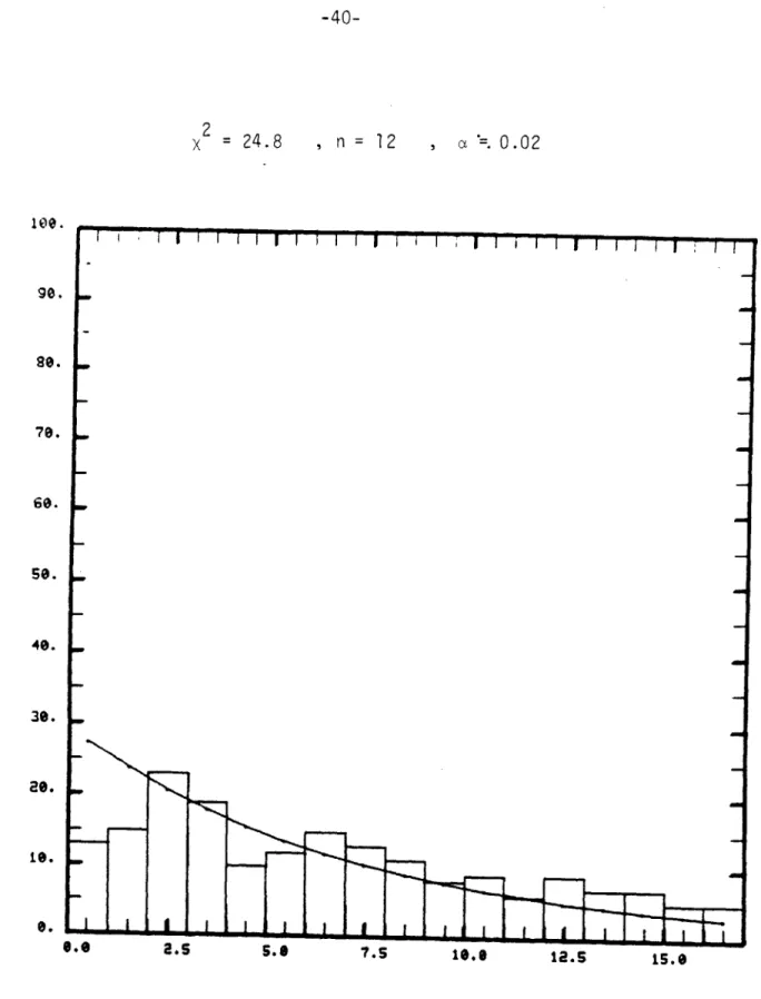
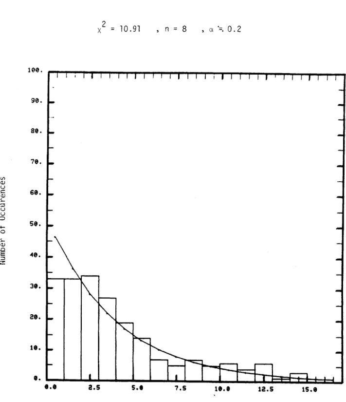
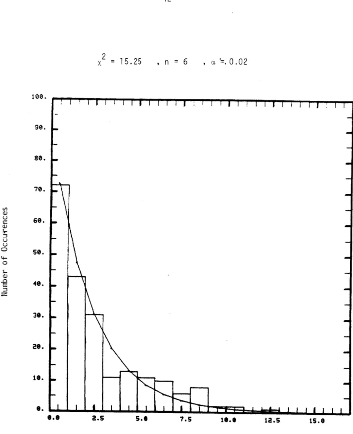
The return values range from 0 to 65025, which is divided into K = 17 intervals and r = 1 because x has been matched to the sample mean. A com-puter program was written to perform the test, with the results given in Figures 12 - 17. In each figure, the bar chart is the histogram of observed frequencies, and the curve is the exponential density fit to the sample mean.

It is not an easy task to explain our results, however some use-ful comments can be made. Data Set 4 has the best fit to the exponential distribution while the others do not fit as well. The fact that Data Set 1 has the worst fit enhances our CCF estimation result ; there is very little randomness in this data set, which was taken in the weakest turbulence. It further convinces us that atmospheric turbulence indeed is an important contributing factor to the return fluctuations, because the atmosphere acts like a "frozen" medium in weak turbulence.

x2 = 43.59

5.0

, n = 6 ef=.0

7.5 _{10.0 12.5 IS.,}

Target-return intensities

Figure 12: Histogram of target-return intensities vs. expected frequencies of Data Set 1.

w C-, C S.-U 4-C S.-100. 90. B0. 70. 60. 5. 45. 30. 2s. 19. 5. I I II I II I Ii II ill I II I I II

.1..

2

x = 18.11 , n = 6 , a _=. 0.005

7.5 _{is.. 12.5 5.e}

Target-return intensity

Figure 13: :Histogram of target-return intensities vs. expected frequencies of Data Set 2.

i

oe.

inL..L

LL

x2 = 24.8 . _b. , n = 12 7.S , '. 0.02 10.1 12.5 _is. Target-return intensities

Figure 14: Histogram of target-return intensities vs. expected frequencies of Data Set 3.

w U a, S.-U U C S.-a, E 1le. 90. 80. 70. 60.

So.

-r

x2 = 10.91

5.0

, n = 8 , a . 2

7.5 1.@ 12.5 Is.0

Target-return intensities

Figure 15 : Histogram of target-return intensities vs. expected frequencies of Data Set 4

90. 80. 70. 60. So. a?) U C--) E S I I I I I~ I I I I I I I I I I I I I I . .P .A ... 40. 3,. 29. 1. 6. .0 2.5

x2 = 15.25 a.5 S.. , n = 6 7.5 , a '=.0.02 10.6 12.5 IS.0 Target-return intensities

Figure 16 :Histogram of target-return intensities vs. expected frequencies of Data Set 5

100. 90. 80. 70. 6e. se.

4e.

in.L

L

je.

2 x =12.21 2.s S., , n = 10 7.5 , a '=. 0.03 19.0 12.5 is., Target-return intensities

Figure 17: Histogram of target-return intensities vs. expected frequencies of Data Set 6

100. 90. BO. 70. 60. So. 40. 39. 20. to. U U 0: 4-0 E iI I I I I I I I I I I I I I I I I J I I I I

..

..

K

CHAPTER III

MATHEMATICAL MODELING

In this chapter we will report on our model for the time

dependence of the staring-mode intensity return fluctuations. The model ascribes the time dependence to random tilts in the radar and target planes. Our first step is to derive a theoretical CCF for staring-mode measurements from the model. Next, because our experimental results have convinced us that atmospheric turbulence is the major cause of the intensity return fluctuationswe use turbulence-induced tilt standard deviations to quantify the.CCF model. The model predictions are then compared with the experimental CCF results. As we shall see, very interesting and significant result is found.

III.1: Theoretical Model

We will model the random radar motion by a random aiming angle error e(t), and the random target motion by a random tilting angle (t). As a result, in the analysis that follows, the transmitted beam and received beam complex envelopes will include the phase term

exp j I(t) - T

and the target reflection process will include the phase term

as shown in Figure 18. The remaining pieces of our radar model parallels that employed in [5], with continuous-wave laser operation and far-field free space propagation assumed.

III.1.1: Model Derivation

1. Let u1 (p,t), the complex envelope of the transmitted laser

beam, be given by,

u(Pt) = (PT) exPp (t) circ2id

where PT is the laser power,

d is the diameter of the exit pupil,

p is the displacement vector on the radar plane, and li(t) is the random aiming error.

2. Let u (P',t) be the transmitted beam complex envelope as it arrives at the target L meters away from the radar. Fraunhofer diffraction theory gives us the result,

exp t7L _{+ 1P 12J}

1!2 (Pt)= jxL dp u pt - exp-

j

where p' is the displacement vector on the target plane. 3. Let u3(p,t), the reflected beam complex envelope at the

UI(, texpp -1

L.O. Beam

Speckle

Target

Figure 18: Radar Configuration

Radar

u3(P' t) = g2(W' t ()exp

F

where (t) is the target tilt angle, and T (p') is a rough surface complex-field reflection function. 4. The complex envelope, u4(p, t), resulting from

propagation back from the target to the radar plane obeys

4(p, 't) = exp j L + jL .

d} d ₃(₉ ', t -

exp

i

-5. Finally, the intermediate frequency complex envelope

(IF) signal has

I.t)

= d 1/2 exp

where e(t) is the aiming error incurred on reception.

Combining the above equations, and using Gaussian beams instead of circular beams to simplify the integrals, we get

y(t) = - exp

j

2

- dp' T (W')exp X (t - )

2 -2 2

7

exp -d

-exp - 21T

XL

2j'~t

exp '

12]

Obviously, the first exponential term in the integration is the moving part of the target reflection model. The second and the third terms are the randomly displaced transmitter beam pattern and the back-propagated local-oscillator pattern, respectively. Our task is to calculate the correlation coefficient function with this IF signal model by assuming statistical properties for T (p') , 6(t) and (t). From this calculation we will be able to see how e(t) and I(t) affect the decorrelation time of the signal intensity fluctuation. Let CCF(T) be the correlation coefficient function, that is

< y_(t + T)I2 |y_(t) 1> - < y(t)j2,2

CCF(t) = _{4 2 2}

<|y(t) >- <ly_(t)I >

Since there is a great deal of tedious algebra involved in deriving CCF, we shall only present the key results here.

The expected value of the IF envelope intensity with respect to the target ensemble is

2 ~ ~P sT Sd P d

JL

<y(t)2T ( ')d

t -

-- 0 P2L ,t2 X

where T (p') has been taken to be a pure speckle target model, i.e., T is a zero-mean circulo-complex Gaussian process with correlation function [5]

<T (P)T*(p2)> = 2 Ts 6(P1 - P2

with Is being the average intensity reflection coefficient of the surface. Assume e(t) is a zero-mean stationary vector Gaussian process with

independent identically distributed components whose: autocovariance function is z(T) = K (T) = K y (k). We then find that,

<ly(t) 2> 2) => << yS 2 T (p' T 2 sT _ _ + 2T 2 d 2 ~z(O) - z

-0 2L .

From this result, we can see that if is short compared with the decorrelation time of z(T), then

<1y(t)K>

P T sd2

2L2

In other words, if F(t) stays constant over times comparable to or

C

longer, the average signal intensity return will be unaffected by the random aiming error ~(t). Note that the average signal intensity is always independent of 6(t), the random tilting angle of the target. The next step is to calculate the quantity,

<_y(t + T)12 jy(t)j 2>,

to be followed by the correlation coefficient function.

Averaging with respect to the target ensemble we get

2

4~dP T2~6t- -t)

<ly(t+-) 2 1iy(t) 2> 2 4 T s -exp -27r2d)2 C

- 4L 4 _2X c _{Td) Ts} 4L 2 _L + 2 + 4 t+----2 t+d2T- 4L + t t+- + - exp {r2d2

eF

L

-51-Next, we average over the (t) ensemble, assuming f(t) to be a zero-mean stationary vector Gaussian process that is statistically independent of

i(t) and has independent identically distributed components whose

autocovariance function is z'(T) = K (T) = K (T). The result we obtain is <<« y(t+)I!y_(t) 2> T S exp>272dd 2 04L~ t - - 2t) 2 t+T- -6(t+T)

L

F1

t

L

16 L

d2j

<Iy(t + T)I2 Iy_(t) I2> = <<<y_(t + T) I

let

Fx(t)

ex

tx t + T

denote a zero-mean Gaussian random vector with covariance matrix

A z(0) (2 L~ zw z(T) Z - TJ z t z(0) z r + z(T) z (T) z 2L IC z

f

z

[?qL

We then have that

<jy(t + T)J2

y(t) 12> = <<<y(t + _) 12 y(t)12>T>_>_ 2 yt)2

I2

C

162L

07

Finally, combining the preceding results for <Iy(t)12> and

<1y(t + T)|2[y(t)jz> we get our predicted CCF

+ ()+ I+2Aw(T)EI II+2 (o)E 1 I+2AW(T)Cl[ d2(z'1 + (o)-z ' (T))+1] JI+ 2Aw(o)CI}

I

-

XJ)

4?

+ 2Tr

d

1

J

]c

I

A substantial simplification results if is much smaller than the

c

decorrelation time of z(t). As our experimental results show decorrelation times of many msec and 2L/c is about 6 ipsec for our data sets, we will set 2L/c = 0 and use the simplified form

CCF(T) =

L(z(o)+z([)) (z(o)-z(-)) + 4(z(o) +

1

16 d 2L2

1

111.1.2: Model Interpretation

To examine the implications of our model we shall assume that the tilt autocovariance functions have the following forms:

Z(T) = T2 e e

and

-T 2/TL

z'(T) = a

e

where Y and ay are the standard deviations of the random radar

aiming error (radar tilt) and the random target motion (target tilt), respectively and Te and -c are the decorrelation times of the radar tilt and target tilt, respectively. We would like to see how the predicted CCF behaves as a function of the dimensionless parameters

Trda

4La

a d

T/Tr and T/T . Intuitively, if ac is larger than N ( > 1), radar

6 e Trd 6

measurements more than T sec apart are likely to illuminate essentially independent portions of the target surface. By the same token, if % > 1 (ay is larger than ), the radar will be likely observed

statistically independent target speckle patterns at time separated by more than T sec.

Let us first consider the behavior of CCF when only one tilt

mechanism is active, i.e., we shall plot CCF vs. T/Te when z'(T) = 0, and CCF vs. T/T4 when z(T) = 0. With these curves, we can compare

the CCF decorrelation time with the decorrelation time of each random tilt.

Case i. z'(T) = 0

In this case, we have that

CCF(T/T ) =

L

which has been plotted in Figure 19 for a = 1,3,5. These curves show that CCF(T/T ) decorrelates faster as a2_{' increases, and for the range}

e e

of a2, shown the GCF decorrelation time is appreciably faster than T.

e e

Case ii. z(T) = 0

In this case, we have

CCF(t/ = / E 4

-which has been plotted in Figure CCF decorrelation time decreases variance increases, but compared CCF decorrelation time is larger decorrelation time.

e }+

]

20 for a = 1,3,5. Once again the as the normalized tilt angle

with the previous figure we see that for the same tilt variance and

0.80 0.70 e.Ge 0.60 CCFs 0.50 0.40 0.30 a - 3 e~ae . 0.0 0*. 0.10 6.20 0.30 0.40 0.s 0.60 0.70 0.80 0.90 1.60 T/Th

* so 0.70 0.60 CCFs 0.40 0.30 0.*20 6.10 0.0 0.16 8.20 8.39 0.40 0.50 0.60 0.70 0.80 0.9, 1.00

Now let us examine how CCF behaves when both tilt mechanisms are present. Here it is worthwhile to define R = T /1e and to

distinguish between R > 1 (radar tilt decorrelates more rapidly than target tilt) and R < 1 (vice versa). In the former case, we will plot CCF vs. T/T6; _{in the latter case we will plot CCF vs.}

T/T .

Case iii. R > 1 In this case, we have

CCF(T/Te) = 71 4(L '' 1+e 1 -

e

{

1

L

I

and 23 give CCF vs. T/Te for the parameter values shown 0

0.10 *.29 0.36 0.40 *.S* 0.60 0.70 0.80 0.90 1.00

T/T

6

Figure 21: Theoretical CCFs with both radar and target tilts active, R > 1 and ae' >

1 .00 0.90 0.80 0.70 0.60 0.50 0.30 0.20 CCFs R= 1 a = 0.1 R= 3 = 3 a '=0.3 R= 5 a ' 0.5 0.6 0..0

o.90 0.80 Rl R = 1 0.60, e.so CCFs 0.40 _{R = 3} a' 3 6.30 _{a 3} * .ae. R= 5 0.1. a 5 0.a' =5 0.0 0.10 *.80 0.30 0.40 *.S@ 0.60 0.70 0.80 . 1.0 T/T 6

Figure 22: Theoretical CCFs with both radar and target tilts active, R > 1 and a₆ ' = a('.

1.00 0.90 0.80 e. 70

o

_e

Figure 23 : Theoretical CCFs with both radar and target tilts active, R > anda < CCFs 0.10 0.20 0.30 R=l a ' e a '=5 R= 3 a '=3 a '-15 R= 5 1 ₅ a =20 .0

Table 3: Parameters for Figures 21, 22, 23 Figure Number 21 22 23 Ratios 1, 3, 5 1, 3, 5 1, 3, 5 a₆ 1, 3, 5 1, 3, 5 1, 3, 5 0.1, 0.3, 0.5 1, 3, 5 5, 15, 20 Case iv. R < I

In this case, we have

e R2 _+4(a')2 { - e $ 2 ₊₇

Figures 24, 25 and 26 give CCF vs. T/T for the parameter values shown in Table 4. CCF(T/T )

4(a

F

{

ei~2

V

N)

{1

1.00 0.80 0.70 0.60 0.40 6.30 0.10 0.0 0. 0.40 6.S0 6.60 0.70 0.80 0.90 1.00

Figure 24: Theoretical CCFs with both radar and target tilts active, R < 1 and a ' < U' 0.10 0.20 0.30 CCFs R = 0.1 a= 0.1 R = 0.2 ' = 0.3 .a R = 0.3 -

a'

0.89 0.70 0.60 0.se 0.40 0.30 *.20 0.10 0. _{0.70 0.86} 0.90 1.00

Figure 25: Theoretical CCFs with both radar and target tilts active, R < 1 anda ' = 1.00 CCFs R 0.1 R = 0.1 R = 0.2 ' = 3 a ' = 3 R =0.3 ae' = 5, (a ' 5 - - . I I I I - I I A - I 0.10 0.20 0.30 0.40 0.50 6.60 0

1.00 0.90 0.80 0.70 0.60 0.50 0.40 0.10 6.6 6. _{6.50 6.60 0.70 6.86 6.96 1.06} T/ T

Fiqure 26 : Theoretical CCFs with both radar and tarqet tilts active, R < 1 and a' > ' CCFs I I I I I I I I I I I

{

Table 4: Parameters for Figures 24, 25, 26

Figure Number Ratios a'

24 0.1, 0.2, 0.3 0.1, 0.3, 0.5 1, 3, 5

25 0.1, 0.2, 0.3 1, 3, 5 1, 3, 5

26 0.1, 0.2, 0.3 5, 15, 20 1, 3, 5

Figures 21-26 reinforce the conclusion drawn earlier from cases (i) and (ii), i.e. the random tilt has a more significant effect than does the target tilt in causing the radar return to decorrelate more rapidly than the tilt itself. Also, as found in cases (i) and (ii), G has to be significantly larger than a to make

these two random effects have comparable impact on CCF. Note that the target is only a calibration plate, which is not as heavy as IRAR. and so the former is more vulnerable to external vibration caused by

the wind. In fact, that is what we will infer in the next section. 111.2. Model Verification

To compare our model with the CCF data from Chapter 2, we need to quantify

Ge,

substituted into our CCF model for comparison with CCF data. By trial and error, however, we have found that to best fit the CCF model to the CCF data the ratio y/a should be made linearly proportional to TeV which is assumed equal to r . As we shall see, this result is

interesting and it allows us to actually predict the decorrelation time of a set of staring data by using the knowledge of the turbulent conditions.

For d < p₀, where d is the diameter of the radar optics exit pupil and p0 is the atmospheric turbulence coherence length, ae can be

computed from [13],

a_{0 2 p5/6 d}1_/6

0

On the other hand, the formula to calculate T needs several steps to develop. It can be shown that in weak turbulence the log-amplitude coherence distance is about equal to /X[ and

T _{~ //vT} '

gives the coherence time of the scintillation in terms of IvTI the magnitude of the tranverse wind velocity which blows perpendicular to the propagation path. Similarly, we have that

PO/IVTI

As a result,

IT5

Finally, p0 is given by,

p = (1.09 C2 k2 L)-3/5

0 n

for a spherical wave [5].

Using the scintillation data from Table 1 and the preceding equations we have obtained the a6 and Te values shown in Table 5.

Table 5: Estimated a and u6 from Turbulence Theory

Data Set No. 1 2 3 4 5 6 a (rad) 4.3 x 10-6 1.3 x 10- 5 1.4 x 10- 5 1.6 x 10- 5 2.1 x 10'5 2.7 x 10 -5 T (ms) & 174.3 27.25 46.8 14.7 18.67 27.2 (pul ses) 3352 524 900 282 359 522

Figures 27-32 show the theoretical and experimental CCF curves for our six data sets assuming a, = (3, Te = T and the values from Table 5.

Obviously, the smooth curve is the theoretical CCF in each figure. At high turbulence levels, Figures 30-32, the theoretical CCFs are very close to the experimental CCFs before the former reaches its asymptotic value. On the other hand, a serious discrepancy occurs in the weak turbulence cases, Figures 27-29. This suggests our model is good

only at high turbulence levels. Also, it leads us to believe turbulence is not the sole factor that causes the tilt effects in our model.

To force the theoretical CCFs to fit the experimental CCFs better, we have tried to vary various parameter values. It was found that if a₆ is kept constant and a is obtained from

jT

G6 110

where T = -- ( measured in pulses) the discrepancy between theoretical CCFs and experimental CCFs is minimized, as shown in

s5. I"*. is"0. 20". as".

PULSES

Figure 27 : Theoretical CCF vs. experimental CCF of Data Set 1.

1.00 *.75 0.50 CCFs e.as 0.0 0. Theoretical CCF Experimental CCF I 1 1 I I I I I I I I 1 I I I I I I I I I I I I I I I I 3000.

1.00

e.

,. 50

500. Is". IS". 20". 2as.

0.

PULSES

Figure 28: Theoretical CCF vs. experimental CCF of Data Set 2. Theoretical CCF

L

50. 1000. IS10. 2090. as*0.

PULSES

Figure 29: Theoretical CCF vs. experimental CCF of Data Set 3.

1.00 0.7s 0.50 CCFs ,.25 0.O Theoretical CCF Experimental CCF 0. 3000.

1 .00 0.75 Theoretical CCF CCFs .. as. Experimental CCF I I I I I I I I I I I I I I I I I I I I I I I

0. See. in*. IS". 20". as**. 3".

PULSES

0.7S

See. 1*. _{is". a29. asse.}

PULSES

Figure 31 : Theoretical CCF vs. experimental CCF of Data Set 5.

I I I I I I I I I I I I I I I I I I Theoretical CCF Experimental CCF I I i i i I i i II I I I 1 I I i i I II I I I CCFs .5as 0.. 0. _3"0.

1.00 0.7S Theoretical CCF *.s

S.

0.7S Theoretical CCF Experimental CCF CCFs *.as 6.S5 I I I I I I I II I I I I I I I I I I I I I I I I 0. S". is". 15". 20W. 25. 3"0. PULSES

Is". IS"0.

PULSES

as*$.

Figure 34: Best CCF fit of Data Set 2. 1.00 0.7s 8.58 CCFs 8.25 0.0 Theoretical CCF Experimental CCF ll 1 111 1i ii I I ii _Ji 0. _as". 30".

1 .00 I II I I I I I I I I I I I I I 0.75 Theoretical CCF 8.se Experimental CCF CCFs *.25. e.g I I I II I I I I I I I I I I I I I I I 1 I I I I I S."0. 10. 1ISO. 20"6. as"0. 30"0. PULSES

1 .00 I i lf lI I II I ~I Pi |7 I I J l i I 0. 75 Theoretical CCF O.se Experimental CCF CCFs *.25. 6.S I I II I I I I I I I I I I I I I I I I I III I

;.e0. i0. ISO$. M"e. as".. 30"e.

PULSES

1.00

0.7

,*se . Theoretical CCF

CCFs ~Experimental _CCF

0.s

o. 5". I I .I 5I. _{20II. as". 39 .}

PULSES

I#". IS". 20S. *

PULSES

Figure 38 : Best CCF fit of Data Set 6.

1.00 0.75 @.S CCFs 0.2 Theoretical CCF Experimental CCF I I I I i I I I I I I I I I I I I I I I I I I I I 0. S".. _{as".. 30".}