Design and analysis of a stage-based electrospray propulsion system for CubeSats

(1)

Design and Analysis of a Stage-Based Electrospray

Propulsion System for CubeSats

by

Oliver Jia-Richards

S.B., Massachusetts Institute of Technology (2018)

Submitted to the Department of Aeronautics and Astronautics

in partial fulfillment of the requirements for the degree of

Master of Science in Aeronautics and Astronautics

at the

MASSACHUSETTS INSTITUTE OF TECHNOLOGY

June 2019

© Massachusetts Institute of Technology 2019. All rights reserved.

Author . . . .

Department of Aeronautics and Astronautics

May 20, 2019

Certified by. . . .

Paulo Lozano

M. Alemán-Velasco Professor of Aeronautics and Astronautics

Thesis Supervisor

Accepted by . . . .

Sertac Karaman

Associate Professor of Aeronautics and Astonautics

Chair, Graduate Program Committee

(2)

(3)

Design and Analysis of a Stage-Based Electrospray Propulsion

System for CubeSats

by

Oliver Jia-Richards

Submitted to the Department of Aeronautics and Astronautics on May 20, 2019, in partial fulfillment of the

requirements for the degree of

Master of Science in Aeronautics and Astronautics

Abstract

The standardization of small spacecraft through CubeSats has allowed for more af-fordable space exploration. This progress in affordability has been limited to Earth orbit due in part to the lack of high ΔV propulsion systems that are compatible with the small form factor. The ion Electrospray Propulsion System developed at the Space Propulsion Laboratory at the Massachusetts Institute of Technology is a promising technology foundation for a compact, high ΔV propulsion system. How-ever, the ΔV output of the propulsion system is limited by the lifetime of individual electrospray thrusters. This thesis presents the design and analysis of a stage-based concept for the ion Electrospray Propulsion System where the propulsion system is composed of a stack of electrospray thruster arrays.

The stage-based propulsion system bypasses the lifetime limit of individual elec-trospray thrusters in order to increase the lifetime of the entire propulsion system. In effect, propulsion capabilities for CubeSats can be advanced without the need for technological developments. With the current performance metrics of the ion Electro-spray Propulsion System, deep-space missions with an initial spacecraft form factor of a 3U CubeSat are feasible with current propulsion technology. Mechanisms required for the stage-based system are designed and demonstrated in a vacuum environment. In addition, analytical methodologies for the analysis of stage-based propulsion sys-tems are developed to assist in preliminary mission design as well as provide the framework for autonomous decision making. Finally, applications of a stage-based propulsion system for missions to near-Earth asteroids are explored as well as ana-lytical guidance for the escape trajectory.

Thesis Supervisor: Paulo Lozano

(4)

(5)

Acknowledgments

Thank you to everyone who has supported me throughout this work. In particular, thank you Paulo for providing me ample opportunity and guidance to develop as an aerospace engineer and trusting me enough to let me work in the Space Propulsion Lab, first as an undergraduate researcher and now as a graduate student. Thank you as well to Emma for always being by my side whether it be writing this thesis, traveling, or watching the Leafs. You have, without a doubt, made my life better and more enjoyable.

Funding for this research was provided by the NASA Space Technology Mission Di-rectorate through the Small Spacecraft Technology Program under grant 80NSSC18M0045 and through a NASA Space Technology Research Fellowship under grant 80NSSC18K1186.

(6)

(7)

List of Figures

1-1 Propellant mass fraction for 3 km/s ΔV mission . . . 18 1-2 Comparison of ΔV versus wet mass for 3U CubeSat propulsion systems 19 1-3 Diagram of electrospray emitter and extractor . . . 20 1-4 iEPS thruster mounted on a single thruster fuel tank . . . 21 1-5 Four iEPS thrusters mounted on the same fuel tank . . . 22 1-6 Configuration of iEPS thrusters on a 3U CubeSat compatible stage. . 23 1-7 Concept image of staging on a 3U CubeSat [10] . . . 25 1-8 ΔV versus wet mass for a 3U CubeSat compatible stage-based system 26 2-1 Diagram of ceramic casing for staging mechanism . . . 29 2-2 Demonstration of staging mechanism in air . . . 30 2-3 Fusing metric for various metals . . . 32 2-4 Effect of capacitor internal resistance on available energy for fusing

given system properties . . . 33 2-5 First resonant mode versus number of stages with 2 or 4 SS304 staging

mechanisms per stage . . . 34 2-6 Proof of concept with early routing mechanism prototype . . . 36 2-7 Stage configuration with staging and routing mechanisms . . . 37 2-8 Test setup for in-air demonstration of staging and routing mechanisms 38 2-9 Demonstration of staging and routing mechanisms with dummy stages

in air with LED’s representing thrusters . . . 38 2-10 Fuse wire after staging mechanism operation in air . . . 39 2-11 Test setup for vacuum testing of staging mechanism . . . 40

(10)

2-12 Demonstration of staging mechanism fusing in vacuum . . . 41

2-13 Capacitor output voltage during staging mechanism test in vacuum . 41 2-14 Capacitor output voltage during staging mechanism fusing in vacuum 42 2-15 Fuse wire after staging mechanism operation in vacuum . . . 42

2-16 Demonstration of staging and routing mechanism with dummy stages in vacuum with LEDs representing thrusters . . . 43

2-17 Test setup for stage-based propulsion system demonstration . . . 44

2-18 Thrusters mounted in custom electronics board . . . 45

2-19 Voltage and current for first stage firing . . . 46

2-20 Thruster plume from first stage firing . . . 47

2-21 Demonstration of a stage-based electrospray propulsion system. . . . 48

2-22 Voltage and current during second stage firing . . . 49

3-1 Ratio of required firing time for escape for velocity pointing and free pointing control laws versus angular pointing control law . . . 53

3-2 Low-thrust escape spiral from Earth without staging . . . 54

3-3 Angular difference between velocity direction and angular direction . 54 3-4 Pareto front for tradeoff in payload mass and escape time . . . 59

3-5 Trajectory, control thrust, and switching function for a 180 day escape trajectory along the Pareto front . . . 60

3-8 Percent error in ΔV approximation versus number of stages . . . 65

3-9 Effect of mass ratio on stage approximation error . . . 66

3-10 Percent error in ΔV approximation versus number of stages when ac-counting for fuel mass flow . . . 68

3-11 Comparison of analytical and numerical calculations of required num-ber of stages neglecting fuel mass flow . . . 70

(11)

3-12 Comparison of analytical and numerical calculations of required num-ber of stages accounting for fuel mass flow . . . 70 3-13 Tradeoff in required number of stages between thrust and stage lifetime

neglecting fuel mass flow . . . 72 3-14 Tradeoff in required number of stages between thrust and stage lifetime

accounting for fuel mass flow . . . 73 3-15 Diagram of different components contributing to the height of a thruster 74 3-16 Mass and volume of a stage-based propulsion system compatible with

the 3U CubeSat form factor based on minimum performance iEPS thrusters . . . 76 3-17 Ratio of firing times for staged to un-staged propulsion systems

ne-glecting fuel mass flow . . . 78 3-18 Ratio of firing times for staged to un-staged propulsion systems

ac-counting for fuel mass flow . . . 79 3-19 ΔV distribution for a stage-based system neglecting fuel mass flow . . 81 3-20 ΔV distribution for a stage-based system accounting for fuel mass flow 82 3-21 Effect of holding partially failed stage before ejecting on ΔV

distribu-tion of the entire propulsion system . . . 85 3-22 Optimal firing time distribution to each stage . . . 92 3-23 Firing time savings from optimal firing time distribution . . . 93 4-1 Comparison of analytical and numerical trajectories for orbit transfer 99 4-2 Percent error in analytical approximation relative to numerical

propa-gation for orbit transfer . . . 100 4-3 Comparison of analytical and numerical trajectories for escape . . . . 101 4-4 Percent error in analytical approximation relative to numerical

propa-gation for escape . . . 102 4-5 Analytical reference trajectory for transfer from a circular

(12)

4-6 LQR feedback controlled trajectory for transfer from a circular medium-Earth orbit to geostationary orbit . . . 112 4-7 Control thrust for LQR feedback controlled trajectory for transfer from

a circular medium-Earth orbit to geostationary orbit . . . 113 4-8 MPC feedback controlled trajectory for transfer from a circular

medium-Earth orbit to geostationary orbit . . . 114 4-9 Control thrust for MPC feedback controlled trajectory for transfer from

a circular medium-Earth orbit to geostationary orbit . . . 114 4-10 Analytical reference trajectory for transfer from a circular low-Earth

orbit to geostationary orbit . . . 115 4-11 LQR feedback controlled trajectory for transfer from a circular

low-Earth orbit to geostationary orbit . . . 116 4-12 Radial position of the spacecraft when using LQR feedback control

starting from a circular low-Earth orbit . . . 116 4-13 Control thrust for LQR feedback controlled trajectory for transfer from

a circular low-Earth orbit to geostationary orbit . . . 117 4-14 MPC feedback controlled trajectory for transfer from a circular

low-Earth orbit to geostationary orbit . . . 118 4-15 Control thrust for MPC feedback controlled trajectory for transfer from

a circular low-Earth orbit to geostationary orbit . . . 119 4-16 Feedforward thrust normalized by maximum thrust of the propulsion

system versus time normalized by the escape time . . . 121 4-17 Feedforward thrust normalized by maximum thrust of the propulsion

system versus time normalized by the escape time when reduced for feasibility . . . 122 4-18 Analytical reference trajectory for escape from Earth starting from

geostationary orbit with reduced reference acceleration . . . 123 4-19 LQR feedback controlled trajectory for escape from Earth starting from

(13)

4-20 Control thrust for LQR feedback controlled trajectory for escape from Earth starting from geostationary orbit with reduced reference accel-eration . . . 125 4-21 Control thrust magnitude normalized by the maximum thrust of the

propulsion system for LQR feedback controlled trajectory for escape from Earth starting from geostationary orbit with reduced reference acceleration . . . 126 4-22 LQR feedback controlled trajectory for escape from Earth starting from

geostationary orbit with partially reduced reference acceleration . . . 126 4-23 Control thrust magnitude normalized by maximum thrust of the

propul-sion system for LQR feedback controlled trajectory for escape from Earth starting from geostationary orbit with partially reduced refer-ence acceleration . . . 127 4-24 Feedforward thrust normalized by the maximum thrust of the

propul-sion system versus time normalized by the escape time when reduced for feasibility and using a stage-based system . . . 128 4-25 LQR feedback controlled trajectory for escape from Earth starting from

geostationary orbit with reduced reference acceleration and a stage-based system . . . 129 4-26 Control thrust magnitude normalized by the maximum thrust of the

propulsion system for LQR feedback controlled trajectory for escape starting from geostationary orbit with reduced reference acceleration and a stage-based system . . . 129 B-1 Initial and goal states for spacecraft . . . 142 B-2 Trajectory solution from model predictive control . . . 144 B-3 Spacecraft trajectory over time with bars representing thruster plumes 145

(14)

(15)

List of Tables

1.1 Performance regimes of iEPS thrusters . . . 22 3.1 Escape time scalar factor for various acceleration ratios . . . 87 3.2 Performance of stage-based propulsion system for escape for minimum

and target iEPS performance metrics . . . 88 4.1 Orbital elements and estimated diameter of easily retrievable objects 96 4.2 Predicted ΔV, required number of stages, and available payload mass

and volume for missions to near-Earth asteroids starting from geosta-tionary orbit . . . 97

(16)

(17)

Chapter 1 Introduction

The standardization of small spacecraft through CubeSats has allowed for more af-fordable space exploration. However, this progress in affordability has often been limited to Earth orbit, with the recent launch of Mars Cube One [1] representing the first deep-space mission performed with CubeSats. There are several other missions that could take advantage of the CubeSat form factor. In particular, missions to near-Earth asteroids lend themselves to the use of CubeSats. Our current under-standing of these asteroids in terms of composition and characteristics is limited and the paradigm of using a single large spacecraft restricts the number of visits to once every few years. By using fleets of CubeSats, all of which could be launched on the same launch vehicle, the frequency of asteroid visits could be dramatically increased all while significantly decreasing the cost per visit.

However, there are a number of technical challenges that are preventing such mis-sions from being performed including the miniaturization of hardware, autonomy, and guidance, navigation, and controls systems. This work aims towards an independent deep-space CubeSat mission from the propulsion standpoint. Specifically, given the current propulsion technology available, can a propulsion system compatible with the CubeSat form factor be developed that can propel CubeSats from Earth orbit into deep-space and to a near-Earth asteroid?

As will be covered in Section 4.1, a mission to a near-Earth asteroid from geo-stationary orbit around Earth will require at least 3 km/s of ΔV when accounting

(18)

Figure 1-1: Propellant mass fraction for 3 km/s ΔV mission

for low-thrust losses. Figure 1-1 shows the propellant mass fraction for a 3 km/s ΔV mission for various specific impulses with typical specific impulses for different propulsion systems marked. Cold gas and chemical monopropellant based propulsion systems are clearly prohibitive for such a mission even if the low-thrust losses were removed. Chemical bipropellant propulsion systems require a fuel mass fraction of 0.53. This is not necessarily a prohibitively high propellant mass fraction given a sufficiently large spacecraft. However, for a 3U CubeSat which has a baseline wet mass of 4 kg, this leaves only 1.88 kg of mass to fit all other aspects of the spacecraft including the nozzle, fuel tanks, and propellant management systems for the propul-sion system, likely preventing the mispropul-sion from being feasible. Therefore, a CubeSat compatible propulsion system capable of producing 3 km/s of ΔV will have to be based in electric propulsion technology.

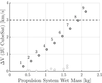
Within electric propulsion, electrospray propulsion holds many advantages that help to reduce the dry mass and volume of the system. Figure 1-2 shows the ΔV capabilities of various 3U CubeSat compatible propulsion systems versus their wet

(19)

Figure 1-2: Comparison of ΔV versus wet mass for 3U CubeSat propulsion systems mass. We can see that all systems fall woefully short of the 3 km/s ΔV requirement with the best system producing 340 m/s of ΔV.

Separate from commercial options, the ion Electrospray Propulsion System (iEPS) developed in the Space Propulsion Laboratory at the Massachusetts Institute of Tech-nology produces relatively high ΔV (second highest of the propulsion systems sur-veyed) with the lowest wet mass. In addition the system occupies a relatively low volume, around 0.5U, for the thrusters, fuel tanks, and power processing unit. The low mass and volume of iEPS is a result of the underlying electrospray propulsion technology and ionic liquid propellant.

1.1 Overview of Electrospray Propulsion

Electrospray thrusters produce thrust through electrostatic acceleration of ions. Ions are evaporated from an ionic liquid propellant by overcoming the surface tension of the liquid with an applied electric field. The ionic liquid propellant is a molten salt at room temperature that is non-reactive, readily available, and has low toxicity. Elec-trospray thrusters and their ionic liquid propellants hold three main advantages that make them an excellent choice for propulsion of small spacecraft such as CubeSats. Firstly, the ionic liquid is “pre-ionized” and does not need an ionization chamber.

(20)

Figure 1-3: Diagram of electrospray emitter and extractor

Second, ionic liquids have near-zero vapor pressure due to the ionic bonds between molecules and therefore do not need any form of pressurized containment. Lastly, propellant is fed to the thruster by passive capillary forces through a porous liner embedded into the fuel tank thereby eliminating the need for any pumping systems. These three advantages allow electrospray thrusters to be incredibly compact and suitable for the CubeSat form factor.

To produce a strong enough electric field to evaporate the ions, the ionic liquid is fed to a sharp emitter tip. A voltage is applied to the ionic liquid with respect to an extractor grid. The sharp tip of the emitter allows for a strong electric field to develop that causes a liquid instability and the development of a sharp liquid meniscus that accentuates the electric field further to the point that ions can be evaporated from the liquid [2]. A diagram of a single emitter and extractor is shown in Figure 1-3. The thrust produced by a single emitter extractor pair is only on the order of 10s of nano-Newtons. Therefore, multiple emitters are arranged in an array to produce a single thruster. Since a single emitter is on the 100 𝜇m scale, arrays of 100s of emitters can be manufactured on a 1 cm scale.

In addition to the inherent advantages of ionic liquid propellants, the operation of electrospray thrusters can also reduce mass and complexity relative to other propul-sion systems. Since the ionic liquid is composed of both positively and negatively charged ions, by changing the polarity of the voltage applied between the emitter

(21)

Figure 1-4: iEPS thruster mounted on a single thruster fuel tank

tip and extractor, the thruster will either evaporate and accelerate negative ions or positive ions. To prevent spacecraft charging, thrusters are operated in pairs with one thruster firing positive ions and the other thruster firing negative ions. This paired operation eliminates the need for a neutralizer further reducing the mass and size of the propulsion system.

1.1.1 ion Electrospray Propulsion System

For this work we will consider the ion Electrospray Propulsion System (iEPS) under development in the Space Propulsion Laboratory (SPL) at the Massachusetts Institute of Technology. Each iEPS thruster consists of an array of 480 emitter tips made from porous glass. The emitter array is housed in a 13 x 12 x 2.4 mm silicon frame with a gold coated silicon extractor grid. Figure 1-4 shows an iEPS thruster mounted on a single thruster fuel tank. Due to the passive propellant feed system, the same iEPS thruster can be mounted on a variety of fuel tanks as long as a porous material connection exists between the ionic liquid and emitter array. Figure 1-5 shows a scaled up configuration where four iEPS thrusters are mounted on the same fuel tank thereby maximizing the density of emitter tips while maintaining structural integrity during launch from Earth.

(22)

Figure 1-5: Four iEPS thrusters mounted on the same fuel tank Table 1.1: Performance regimes of iEPS thrusters

Minimum Target

Max thrust 20 𝜇N 80 𝜇N

Specific impulse 1000 s 2500 s

Lifetime 500 hr 1000 hr

impulse close to 1000s when using EMI-BF4 as the ionic liquid propellant [3].

How-ever, the thrust and specific impulse are heavily dependent on the ionic liquid used as well as the material of the emitter array. Ongoing research at the SPL is investigating different materials for the emitter array that can contribute to an increased thrust, specific impulse, and thruster lifetime [4]. Two regimes of thruster performance are considered throughout this work. The first represents the current demonstrated per-formance which is the minimum expected perper-formance of the thrusters during imple-mentation. The second represents the target performance which is based on expected near term developments. The performance metrics for both the minimum and target performance regimes are summarized in Table 1.1.

A single iEPS thruster on its own does not produce enough thrust to be useful for main propulsion of a CubeSat mission. While the low thrust has other applica-tions, such as for high precision attitude control [5], for main propulsion the thrust is increased by using arrays of thrusters. Tanks with four thrusters each, as shown in Figure 1-5, are arranged on a 1U CubeSat face. A 1U CubeSat face can hold up to nine of these clusters in a 3 x 3 square pattern for a total of 36 thrusters. For this

(23)

Figure 1-6: Configuration of iEPS thrusters on a 3U CubeSat compatible stage. work, we will consider a configuration where a thruster in the center row is omitted to provide space for the staging electronics, which will be introduced in Section 1.2, and mounting on either side of the thrusters as shown in Figure 1-6.

This configuration, with 32 thrusters, can produce 0.64 mN of thrust in the mini-mum performance case and 2.56 mN of thrust in the target performance case. While this thrust is still relatively small, the low mass of the CubeSat form factor means that the net acceleration is comparable to that of other electric propulsion based missions such as Dawn [6].

1.1.2 Lifetime Limitations of Electrospray Thrusters

While electrospray thrusters are highly compatible with the CubeSat form factor due to their mechanical simplicity and small size, the ΔV that can be produced by an electrospray thruster based system is limited by the operational lifetime of the thrusters themselves. The primary life-limiting mechanism for electrospray thrusters is accumulation of propellant on the extractor grid [7]. The beam of ions which is extracted from the emitter tip leaves in a conical shape with observed half-angles of 60 degrees [3]. The beam can therefore impact the extractor grid and allow propellant to

(24)

accumulate or backspray onto the emitter array. Misalignments between the emitter tips and extractor grid during thruster manufacturing can accentuate the impingment of the ion beam onto the extractor grid and increase the rate at which propellant accumulates. If enough propellant accumulates, an ionic liquid connection can be formed between the emitter and extractor causing an electrical short and rendering the thruster inoperable. It is believed that propellant accumulation caused an electrical short of one of the electrospray thrusters on the ESA LISA Pathfinder mission [8].

While ion beam impingement with the extractor grid is the primary lifetime lim-itation of electrospray thrusters, there are many other effects that can contribute to a reduced lifetime. Models as well as experimental techniques to analyze the var-ious lifetime limitations are developed in [7] and [9] and, as mentioned prevvar-iously, efforts are being made to increase the lifetime of current iEPS thrusters. However, in the near term future, even if the target performance metrics for iEPS thrusters are met the thrusters will not have sufficient lifetime to produce enough ΔV to conduct deep-space missions. In addition, even if the lifetime of the thrusters were infinite, a stage-based approach provides multiple other benefits such as propulsion system redundancy or the potential for new avenues of mission optimization.

1.2 Staging Concept

To increase the ΔV output of an electrospray thruster propulsion system, the lifetime limitation has to be overcome. While the lifetime of electrospray thrusters will in-crease as the technology matures, increasing the lifetime to the point where 3 km/s of ΔV could be produced would take a substantial amount of development. Therefore, in order to enable deep-space, and more generally high ΔV, missions with Cube-Sats, an alternative method needs to be developed that bypasses the lifetime limit of an individual electrospray thruster in order to increase the overall lifetime of the propulsion system.

A staging concept is proposed where the propulsion system consists of a series of stages of electrospray thruster arrays. Figure 1-7 shows a concept image of the

(25)

Figure 1-7: Concept image of staging on a 3U CubeSat [10]

staging system on a 3U CubeSat. As an array of electrospray thrusters reaches its lifetime limit, it is ejected from the spacecraft exposing a new array of thrusters in order to continue the mission. With such a system, the lifetime limit of an individual electrospray thruster is bypassed and the lifetime of the overall propulsion system can be arbitrarily increased by increasing the number of stages.

In terms of the ΔV production, Figure 1-8 shows the ΔV versus wet mass for a stage-based system with one to nine stages. We can see that a nine stage system can provide enough ΔV to complete the mission and has mass low enough that the system is compatible with the CubeSat form factor. As will be shown in Section 3.2.4, the volume of the nine stage propulsion system is 2.1U leaving enough mass and volume

(26)

Figure 1-8: ΔV versus wet mass for a 3U CubeSat compatible stage-based system for a small, but capable, mission.

The remainder of this thesis is dedicated to the design, analysis, and application of a stage-based electrospray propulsion system. Chapter 2 covers the design of the mechanisms for a stage-based propulsion system as well as their testing in a vacuum environment and integration with actual thrusters for a full laboratory demonstration of a stage-based propulsion system. Chapter 3 analyzes a stage-based system from an analytical approach and develops methodologies for preliminary propulsion system and mission analysis with stage-based systems and the framework for autonomous decision making on small spacecraft with stage-based propulsion systems. Chapter 4 looks at the application of stage-based propulsion systems for missions to near-Earth asteroids as well as extensions of analytical methodologies for analytical guidance of spacecraft performing orbit transfers and escape missions enabling complex missions to be performed with computationally simple reference trajectories.

(27)

Chapter 2 Design

Two approaches could be used to increase the total lifetime of the propulsion sys-tem. Either the lifetime of individual thrusters could be increased, or an alternative system could be developed that bypasses the lifetime limit of the thrusters. Near-term developments at the SPL aim to increase the lifetime of individual thrusters through improvements in materials and manufacturing techniques. However, those developments only expect to increase the lifetime by a factor of 2 or 3, still less than the required firing time to enable deep-space missions from geostationary orbit. In addition, even if the lifetime of the thrusters were infinite, a stage-based approach opens up new avenues for mission optimization similar to the optimization of launch vehicles. Therefore, a staging concept is proposed with sequential stages of thruster arrays. One set of thrusters is fired until the lifetime limit before being ejected from the spacecraft and exposing a new set of thrusters. Through staging, the lifetime limit of individual thrusters is bypassed in order to increase the overall lifetime of the propulsion system. Figure 1-7 shows a concept image of a stage-based system and a CubeSat staging a set of thrusters mid-flight.

Development of a staging concept also provides two additional benefits. Firstly, stages can be used to provide redundancy for the propulsion system. Second, as thrusters are fired they might, after some time, decay and their performance decreases. Current efforts to minimize the effect of this decay involve increasing the input voltage to the thruster [11]. However, increasing the input voltage further accelerates thruster

(28)

decay and requires more power. By staging thrusters, a new, fresh set of thrusters will be used thereby avoiding the effects of thruster degradation.

Normally, this staging concept would not be feasible for most propulsion systems. However, the compact nature of iEPS thrusters and the lack of need for ionization chambers, pressurized propellant containment, and propellant feed systems means that the contribution of a single thruster array to the overall spacecraft mass and volume is small relative to other spacecraft systems. A complete array of thrusters compatible with a 3U CubeSat with enough fuel for 500 hours of firing only occupies approximately 0.2U (200 cm3_{) of volume and weights 220 grams.}

To develop the stage-based propulsion system, two mechanisms are required. The first is the staging mechanism itself which holds together successive stages during flight and separates the outermost stage at the time of staging. The second is a routing mechanism that passively routes control signals to the active stage. All thruster stages will use the same control electronics. Therefore, it is necessary to route the control signals to the correct stage. By performing the routing mechanically and passively, the control electronics can remain “stage-blind” and no electrical addressing of individual stages will be required. Both mechanisms are designed, prototyped, and demonstrated in a vacuum environment with iEPS thrusters to demonstrate a stage-based propulsion system.

2.1 Staging Mechanism Design

The staging mechanism is based on a fuse wire approach. Successive stages are held together with a thin stainless steel wire. At the time of staging, a high current (10 A) provided by a high power density (≤ 200 mΩ ESR) ultra-capacitor is run through the wire, heating it up until it melts. After the wire melts and the stages are separated, a compression spring is used to eject the stage from the spacecraft. The wire is housed in a ceramic casing and attaches to standard 4-40 standoffs allowing for easy integration to existing iEPS electronics boards.

(29)

Figure 2-1: Diagram of ceramic casing for staging mechanism

composed of two ceramic casings both with their spring housings facing inwards. A 0-80 screw terminal is used to hold the stainless steel wire under tension due to the compressed spring and to provide electric contacts for the capacitor. The slot for the fuse wire is slightly off center such that when the fuse wire is held in the slot, the wire itself is centered in the ceramic casing. A 4-40 threaded hole is included at the back of the casing for mounting. Figure 2-2 shows the staging mechanism in operation. The entire fusing procedure takes approximately 100 ms. A gap between the ceramic casings is intentionally added during this test in order to provide visibility to the fuse wire. During normal operation, the ceramic casings are flush.

Similar approaches have been explored previously for miniature release mecha-nisms for small satellites. A nichrome burn-wire mechanism is explored in [12] where a nichrome wire is heated up in order to cut through a Vectran tie down cable. The release mechanism in this research differs from [12] in that the wire itself is melted to activate release rather than used to cut through a second wire therefore simplifying the mechanism design.

Multiple miniature release mechanisms are explored in [13] including a fuse wire based mechanism. The fuse wire mechanism in [13] is based on a beryllium-copper wire and has the wire loop through a retainer mechanism. The mechanism in [13] uses five unique components and requires the fuse wire to be etched in order to control the fusing location. The mechanism developed in this research keeps the fuse wire

(30)

(31)

straight and uses four unique components, only one of which, the ceramic casing, requires fabrication. By keeping the wire straight and securing it between two screw terminals, no wire etching is required as the wire can fuse in any location and still release the two stages.

2.1.1 Fuse Wire Material Selection

Material selection for the fuse wire consists of balancing mechanical and thermal properties. Desirable mechanical properties are low density and high tensile strength while desirable thermal properties are low specific heat capacity and low melting point. These properties can be combined to form a fusing metric, Γ, which is a function of the wire’s initial temperature and defined as

Γ(𝑇0) ≡

𝜌 𝑐 (𝑇m− 𝑇0)

𝜎 (2.1)

where 𝜌 is the wire’s density, 𝑐 is the specific heat capacity, 𝑇m is the melting point,

𝑇0 is the initial wire temperature, and 𝜎 is the ultimate tensile strength. The fusing

metric is also equal to the ratio of the required energy to fuse the wire, 𝐸f, to the

maximum load the wire can carry, 𝐹 , and the length of the wire, 𝑙 Γ ≡ 𝐸f

𝐹 𝑙 (2.2)

For a given maximum load and wire length, set by the form factor of the spacecraft and staging mechanism, the fusing metric gives the minimum energy required for fusing before losses. Materials with a lower fusing metric are therefore more desirable.

Figure 2-3 shows the ultimate tensile strength versus the fusing energy per unit volume for various materials starting from an initial temperature of 0° C. Lines orig-inating from the origin represent lines of constant fusing metric with lines with a larger slope correspond to lower fusing metrics. The line for Γ = 10 is shown for reference. Per this analysis, good material choices are the stronger aluminum and beryllium-copper alloys. In addition, pure tin is a particularly good choice with a

(32)

Figure 2-3: Fusing metric for various metals fusing metric of 1.3.

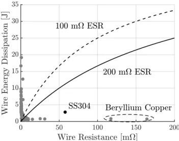
Beyond mechanical and thermal properties, the electrical properties of the mate-rial determine its ability to be integrated into the spacecraft system. While pure tin has a low fusing metric, its low conductivity prevents its use given current capacitor capabilities. A 6.35 mm long pure tin wire capable of holding 40 N of force has a resistance an order of magnitude lower than the internal resistance of commercially available high power density capacitors (∼200 mΩ ESR). This discrepancy in resis-tance prevents power dissipation in the wire and therefore prevents fusing. Figure 2-4 shows the available energy output from a capacitor with energy capacity of 50 J and internal resistance of 200 mΩ. Required energies for fusing for materials shown in Figure 2-3 as well as total wire resistances are shown for 6.35 mm long wires capable of holding 40 N of load (equivalent to 4 wires each holding 10 N of load). We can see that most materials have very low resistances (∼5 mΩ) due to their low resistivity and therefore do not dissipate enough energy for fusing.

For this work, stainless steel 304 (SS304) is used as the fuse wire material. Al-though SS304 has a poor fusing metric (∼11) we can see from Figure 2-4 that its relatively high resistivity means that more of the capacitor energy is dissipated in the wire compared to most other materials considered in this study thereby allowing for wire fusing with sufficient safety margin. In addition, SS304 is readily available

(33)

Figure 2-4: Effect of capacitor internal resistance on available energy for fusing given system properties

which allows for rapid prototyping. As capacitors with lower internal resistances are developed, materials such as tin which offer better fusing metrics can be used. Figure 2-4 also shows the available energy for fusing if the internal resistance of the capacitor is reduced by half to 100 mΩ.

Select beryllium-copper alloys are the only materials surveyed that have lower required fusing energy and higher wire resistance than SS304. However, given that SS304 is more readily available and can be fused with the capacitor considered in this study, SS304 is used for all tests in the in this work. Future work will consider using beryllium-copper alloys as the fuse wire material.

The fuse wire itself is 6.35 mm long and has a diameter of 0.203 mm (0.008 in). Each fuse wire can therefore hold ∼16 N of load. Given the fusing metric of SS304 ∼11, the estimated energy to fuse the wire is 1.15 J. As the melting point of SS304 is high (1400° C) the effect of initial wire temperature is minimal and so a reference of 0° C is used.

2.1.2 Vibration Analysis

With the addition of the staging mechanism, successive stages are only held together by 2-4 thin metal wires thereby influencing the vibration characteristics of the

(34)

space-Figure 2-5: First resonant mode versus number of stages with 2 or 4 SS304 staging mechanisms per stage

craft during launch. While the entire spacecraft structure could be constrained, in the worst-case scenario the entire vibrational load will have to be absorbed by the fuse wires.

The stack of stages is approximated by stacked spring-mass systems where the spring constant, 𝑘, is approximated as

𝑘 = 𝑁𝐴 𝐸

𝐿 (2.3)

where 𝑁 is the number of staging mechanisms per stage, 𝐴 is the wire cross-sectional area, 𝐿 is the relaxed wire length, and 𝐸 is the Young’s modulus of the wire material, SS304 in this case. Figure 2-5 shows the first resonant mode of the staging stack versus number of stages for both 2 and 4 SS304 staging mechanisms per stage. In all cases, the first resonant mode is greater than 100 Hz and will therefore avoid dynamic coupling between the low frequency dynamics of the launch vehicle and the stages.

In actuality, the first resonant modes will be higher than in this analysis. The spring-mass approximation allows for compression of the fusing wire. On the staging mechanisms, compression of the fusing wire is constrained by the stiffer machinable ceramic casing. Future work will involve experimental measurement of the resonant

(35)

modes of the staging mechanisms as well as their response to random vibration.

2.2 Routing Mechanism Design

The routing mechanism is a custom made, normally closed, momentary push button switch. When a preceding stage is present, the mechanism is opened preventing control signals from entering the stage. When the preceding stage is ejected, the mechanism is closed and the stage becomes active. After the thrusters on the stage reach the end of their lifetime, the stage is ejected, automatically activating the next stage. With this mechanism the control electronics remain “stage blind” and do not need to track which stage is active. This greatly simplifies the electronics design as existing iEPS electronics boards can continue to be used without needing to add extra electronics for addressing of individual stages. It also allows for greater flexibility when adding or removing stages as the number of stages does not impact the electronics boards.

Figure 2-6 shows a proof of concept of the routing mechanism concept with an early routing mechanism prototype. We can see that without any actuation, the contacts between the two ends of the routing mechanism are connected and the multimeter reads a finite resistance. When the mechanism is actuated, through pushing down the button, the connection between the contacts is broken and the multimeter is overloaded as it cannot read a finite resistance. When integrated into a stage-based propulsion system, each stage will physically actuate the routing mechanism for the stage below it. The button will be pressed down by the stage board such that when the above stage is present the routing mechanism is inactive (connection between contacts broken) and when the above stage leaves, the routing mechanism becomes active (contacts are connected).

(36)

(37)

Figure 2-7: Stage configuration with staging and routing mechanisms

2.3 Stage Configuration

Both the staging and routing mechanisms can be easily integrated onto the proposed stage configuration in Figure 1-6. The staging mechanisms simply replace the 4-40 standoffs used for mounting and the routing mechanisms can be added in the spaces next to the center row of thrusters. Figure 2-7 shows the thruster configuration with the routing mechanisms included and with the mounting holes replaced with staging mechanisms. All control electronics required for thruster firing and staging mechanism activation will be mounted on separate electronics boards below the stage stack and have their signals routed to the active stage through the routing mechanisms.

2.4 Mechanism Testing

Testing of the stage-based system is conducted first in air and then in vacuum. Figure 2-8 shows the test setup for an in-air demonstration of the staging and routing mech-anisms with dummy stages. Two staging mechmech-anisms are used for the test and are fused with a PBL-4.0/5.4 passively balanced ultracapacitor from Tecate Group. The control electronics first charge the capacitor to at least 4.4 V before fusing the staging mechanisms. An LED is included on each stage to represent electrical connections for thrusters with a common power connection run through the routing mechanism. We can see that in the initial setup, the LED on the first stage is lit since it is the

(38)

Figure 2-8: Test setup for in-air demonstration of staging and routing mechanisms

Figure 2-9: Demonstration of staging and routing mechanisms with dummy stages in air with LED’s representing thrusters

active stage while the LED on the second stage is not lit.

Figure 2-9 shows the in-air demonstration. In the first image, the system is in the initial configuration as shown in Figure 2-8. In the second image, the staging mechanisms are activated. We can see the glow from the fuse wires as the first stage is ejected. In addition, the LED on the second stage is now lit as the contacts on the routing mechanism are closed when the first stage is ejected. In the final image, the first stage is fully ejected and the second stage is now active. The LED on the second stage remains lit, representing the second array of thrusters now firing.

(39)

Figure 2-10: Fuse wire after staging mechanism operation in air

2.4.1 Vacuum Testing

To mature the stage-based propulsion system technology, the staging system needs to be tested in a vacuum environment. Since the routing mechanism operation is entirely mechanical, there is no expected difference in operation in air versus vacuum. However, the behavior of the fusing mechanism might have minor differences. Figure 2-10 shows the fuse wire after staging mechanism operation in air. We can see that the wire has oxidized around the fusing point due to the high heat and the break in the wire looks more like the wire snapped rather than melting.

The test setup for testing the staging mechanism in a vacuum chamber is shown in Figure 2-11. The same PBL-4.0/5.4 ultracapacitor from Tecate Group is used and a relay controls whether or not the capacitor is charging or the staging mechanism is fusing. No spring is included in the staging mechanism during this test to prevent debris in the vacuum chamber. Figure 2-12 shows the staging mechanism operating in vacuum at 𝜇Torr levels. The green LED in the first image indicates that the capacitor is charging while the yellow LED in the second image indicates that the staging mechanism is being fused. We can see the fuse wire in the staging mechanism

(40)

Figure 2-11: Test setup for vacuum testing of staging mechanism glowing during operation as expected.

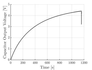
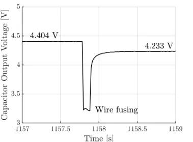
Figure 2-13 shows the capacitor output voltage throughout the test. We can see that the capacitor charges to 4.4 V in just over 19 minutes, requiring an average power input from the spacecraft bus of only 0.05 W. After the capacitor voltage reaches 4.4 V, the electrical connection from the power supply to the capacitor is broken and the capacitor is electrically connected to the staging mechanism to initiate fusing. Figure 2-14 shows the portion of the voltage plot in Figure 2-13 corresponding to fusing. We can see a drop in output voltage due to the equivalent series resistance of the capacitor. The fuse wire fuses in approximately 100 ms after which the capacitor output voltage recovers to its final value of 4.2 V. Energy wise, 4 J of energy are used during the fusing which is split between the fuse wire and the internal resistance of the capacitor. Figure 2-15 shows the fuse wire after staging mechanism operation in vacuum. In contrast to the fuse wire that was operated in air in Figure 2-10 we can see that no oxidation occurred, due to the lack of air, and that both sides of the fuse wire have clearly melted at the fuse point in order to cause the separation of the staging mechanism.

(41)

Figure 2-12: Demonstration of staging mechanism fusing in vacuum

(42)

Figure 2-14: Capacitor output voltage during staging mechanism fusing in vacuum

(43)

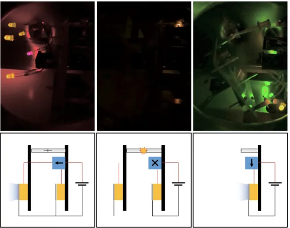
Figure 2-16: Demonstration of staging and routing mechanism with dummy stages in vacuum with LEDs representing thrusters

test with dummy stages similar to the in-air test in Figure 2-9. Figure 2-16 shows the combined test in vacuum at 𝜇Torr levels with LEDs as electrical placeholders for thrusters. The lighting in the chamber was dark throughout the test in order to properly see the visual cues, such as when the staging mechanism was activated. Therefore, a diagram is provided below the test sequence showing what is happening in the chamber throughout the test on an electrically equivalent thruster system.

The test used a two stage system with a common power supply for both stages. Initially, when both stages are present, the power for the LEDs is routed past the second stage and up to the first stage. We can see, in the first image, that the LEDs for the first stage are lit in this initial configuration and that the thruster on the first stage is firing in the supplemental diagram. After the first stage reaches its lifetime limit the staging mechanisms are activated. The electrical connection to the first stage is cut, visually demonstrated by the LEDs on the first stage no longer

(44)

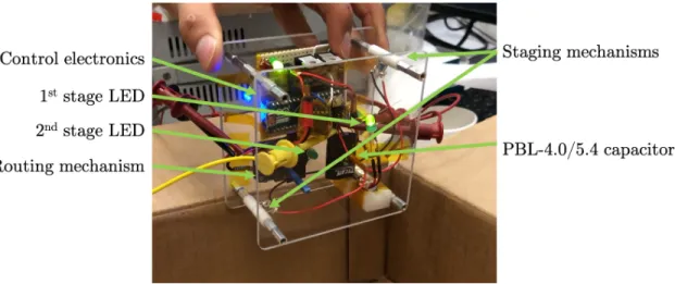
Control electronics for staging Thruster power processing unit 2nd_stage 1st_stage Staging mechanisms Routing mechanisms

Figure 2-17: Test setup for stage-based propulsion system demonstration lit up, and the electrical connections to the second stage are still not closed. The staging mechanism fuse wires are glowing as the mechanisms are activated in order to initiate staging. After staging has been completed, the first stage is ejected from the spacecraft activating the routing mechanism on the second stage and closing the associated electrical connections. The LEDs on the second stage are now lit representing the second stage thrusters now firing.

2.4.2 Fully Integrated Test

Figure 2-17 shows the test setup for testing of the staging and routing mechanisms with electrospray thrusters. The test used the already existing iEPS power processing unit with custom control electronics for the staging as well as custom thruster boards to hold two thrusters and to accommodate the routing mechanisms. During the test, aluminum foil was wrapped around the thruster power processing unit and staging control electronics in order to prevent potential charging due to reflection of emitted ions from the vacuum chamber walls. Figure 2-18 shows the thrusters mounted on one of the thruster boards prior to testing.

Figure 2-19 shows the voltage and current output when firing the first stage. We can see that emission was achieved in the ∼900 V range. The thrusters were

(45)

Figure 2-18: Thrusters mounted in custom electronics board

operated at 1000 V for three 30 second polarity cycles. We can see a significant asymmetry in the current levels between the two thrusters and also when the thruster polarities are switched. The thrusters were operated at a higher-than-intended current level. However, due to the high current level, Figure 2-20 shows a visible plume from the thrusters confirming that the thrusters were actually firing during the test. Unfortunately, the thrusters were left not firing over night and developed an electrical short by the morning. It is suspected that the short was due to gravity pulling the ionic liquid towards the edge of the emitter array and creating an electronic connection between the emitter array and extractor grid.

Since the first stage was deemed inoperable, it was staged from the propulsion sys-tem. Figure 2-21 shows the staging sequence. Initially, both stages are still attached to the propulsion system. The staging mechanisms are then activated and the first stage is ejected from the system. After staging, the propulsion system is left with only the second stage and is ready to continue thruster firing.

Figure 2-22 shows the voltage and current output when firing the second stage. The vast majority of the perceived noise in the output is due to switches in the thruster polarity. Unfortunately, only one of the two thrusters on the second stage successfully fired. The unfired thruster initially showed no signs of firing when a voltage was

(46)

(47)

Thruster plume

Figure 2-20: Thruster plume from first stage firing

applied before developing an electrical short rendering it inoperable. However, the thruster that did fire fired as expected in terms of output current. An emitted current of 150 𝜇A was achieved and maintained for almost ten hours. Approximately ten hours into the test, a voltage trip caused the PPU to stop applying voltage to the thruster causing the thruster to sit not firing over night and developing an electrical short similar to what happened with the first stage.

This test serves as the first demonstration of a stage-based electrospray propulsion system. Electrospray thrusters on two different stages were fired and the first stage was successfully ejected from the propulsion system. While thrusters were rendered inoperable throughout the test, the causes do not appear to be associated with the stage-based propulsion system. In addition, all thrusters used for this test were test units and not engineering or flight units so unexpected behavior, such as premature shorting, was to be expected. Further refinement of both the staging and routing mechanisms is required to make the system flight ready. However, the mechanical feasibility of such a propulsion system has been demonstrated.

(48)

(49)

(50)

(51)

Chapter 3 Analysis

3.1 Un-staged Escape Trajectory

Before analyzing trajectories with stage-based propulsion systems, it is worth analyz-ing trajectories of un-staged propulsion systems to first determine what control law and thrust program to use during escape. Specifically, there are two questions we aim to answer with this analysis:

• What control law should be used (what direction to apply thrust)? • Should coast arcs be added to the trajectory to improve payload mass?

To determine the control law to use, three control laws are considered: angular pointing, velocity pointing, and free pointing. Angular pointing and velocity pointing mean that the thrust is constrained to be applied in the angular and velocity directions respectively. In free pointing, the thrust direction is left free and is optimized with the GPOPS-II general purpose optimal control software [14]. Of the three options, angular pointing and velocity pointing are considerably simpler control laws in regards to implementation on a small satellite. Angular pointing provides the additional benefit of maintaining a face of the satellite pointed at Earth which can be useful for navigation purposes. We will find that velocity pointing and free pointing do not provide any significant advantages over angular pointing in terms of escape time. Therefore, angular pointing will be the control law of choice.

(52)

The addition of coast arcs in the trajectory allows for a tradeoff between payload mass delivered to escape and escape time. Optimal control with calculus of variations is used to determine when to add coast arcs into the trajectory in order to maximize the payload mass delivered to escape for a given escape time. Calculus of variations allows the problem to be reduced from an optimization of a continuous time variable, the thrust input, down to an optimization over a few scalar values. However, the result of the optimization will give that adding coast arcs to the trajectory only provides marginal increases in the payload mass while requiring significant increases in escape time. Therefore, the final control law will be angular pointing with no coast arcs (continuous thrust).

3.1.1 Comparison of Control Laws

Three control laws are considered for the escape trajectory: angular pointing, velocity pointing, and free pointing. In all cases, thrust is applied continuously throughout the trajectory, then the three control laws are then compared based on the firing time required to achieve escape from geostationary orbit. Angular pointing and velocity pointing are easily evaluated by propagating the trajectory with their respective con-trol law. For free pointing, the GPOPS-II general purpose optimal concon-trol software [14] is required in order to optimize the direction of thrust to minimize the required firing time.

Figure 3-1 shows the ratio of firing time for escape for the velocity pointing and free pointing control laws versus the angular pointing control law for various thrusts normalized by the iEPS minimum performance value. We can see that the velocity pointing and free pointing control laws provide marginal improvements in escape time compared to angular pointing with a maximum decrease in escape time of ∼1.35%. In addition, we can see that there is almost no difference between the velocity pointing and free pointing results.

The marginal difference between angular pointing and velocity pointing is due to the nature of the low-thrust escape spiral. Figure 3-2 shows the escape spiral for the minimum performance iEPS thrust along with the orbit of the Moon for scale. We can

(53)

Figure 3-1: Ratio of required firing time for escape for velocity pointing and free pointing control laws versus angular pointing control law

see that except for the last revolution of the spacecraft around the Earth, the orbit is approximately circular. Therefore, there is little difference between the velocity pointing and angular pointing control laws. We can see this more clearly in Figure 3-3 where the angular difference between the velocity direction and angular direction is plotted over time. For the vast majority of the trajectory the two directions are nearly aligned with an angular difference of only ∼4.5 degrees after 75% of the trajectory has been completed.

The small difference between the velocity pointing and free pointing control laws is also not surprising. If we consider the specific power input of the propulsion system to the spacecraft

𝑑𝜖 𝑑𝑡 =

1

𝑚𝐹 · ⃗⃗ 𝑣 (3.1)

where 𝜖 is the specific energy of the orbit, 𝑚 is the mass of the spacecraft, ⃗𝐹 is the thrust vector, and ⃗𝑣 is the velocity vector, then we can see that the instantaneous change in the specific energy of the orbit is maximized if the thrust vector is aligned with the velocity vector. If the goal of the mission is to achieve escape (𝜖 → 0) then the intuitive control law would be to align the thrust and velocity vectors - velocity

(54)

Figure 3-2: Low-thrust escape spiral from Earth without staging

(55)

pointing. The free pointing optimization can only make marginal improvements to the velocity pointing control law by sacrificing the instantaneous change in specific energy to slightly improve the change in specific energy at a later time in the trajectory.

Implementation wise, the free pointing control law is more complex than either the velocity pointing or angular pointing control laws and is susceptible to model-ing errors. Both the velocity pointmodel-ing and angular pointmodel-ing control laws are simple to implement assuming knowledge of the spacecraft velocity vector. However, the angular pointing control law has the additional bonus that a face of the spacecraft will always be pointed towards Earth throughout the escape trajectory. This can be advantageous for communications and autonomous navigation. The spacecraft’s radial position can be estimated by taking measurements of the angular diameter of the Earth during escape. In addition, the angular position of the spacecraft can be estimated by combining measurements from a star tracker and the position of the Earth in the spacecraft’s camera. Therefore, while the velocity pointing control law does have a lower escape time than the angular pointing control law, angular pointing will be the default control law for future analysis.

3.1.2 Optimization with Calculus of Variations

In Section 3.1.1 angular pointing was selected as the control law but the analysis assumed constant thrust applied throughout the trajectory. Here, we are interested in optimizing our trajectory to minimize propellant mass usage by allowing for vary-ing thrust throughout the trajectory. The goal of this analysis is to determine the tradeoff between escape time and propellant mass - can we save a significant portion of propellant mass by taking a little longer to reach escape? It is worth noting that this problem is a restricted form of Primer Vector Theory which is covered in [15].

Formally, the problem can be expressed as min 𝐹 (𝑡) 𝐽 =propellant mass = ∫︁ 𝑡𝑓 0 𝐹 (𝑡) 𝑐 𝑑𝑡 (3.2)

(56)

subject to the dynamics ˙𝑟 = 𝑣𝑟 (3.3) ˙ 𝜃 = 𝑣𝜃/𝑟 (3.4) ˙𝑣𝑟 = 𝑣2𝜃/𝑟 − 𝜇/𝑟2 (3.5) ˙𝑣𝜃 = −𝑣𝑟𝑣𝜃/𝑟 + 𝐹/𝑚 (3.6) ˙ 𝑚 = −𝐹/𝑐 (3.7)

saturation limits for the input thrust

0 ≤ 𝐹 ≤ 𝐹max (3.8)

and the final condition that the spacecraft must achieve escape 1 2(︀𝑣 2 𝑟+ 𝑣 2 𝜃)︀ − 𝜇 𝑟 ≥ 0 (3.9)

We can solve this problem with optimal control using calculus of variations. A good reference for the derivation of the necessary conditions for optimal control is [16]. Here, we will advance the results of the derivation and form the Hamiltonian function by combining our cost function with our dynamics adjoined with costate variables 𝜆

𝐻 = 𝐹

𝑐 + 𝜆𝑟˙𝑟 + 𝜆𝜃 ˙

𝜃 + 𝜆𝑣𝑟˙𝑣𝑟+ 𝜆𝑣𝜃˙𝑣𝜃+ 𝜆𝑚𝑚˙ (3.10) where the time dependences of all variables has been dropped for clarity. Substituting in the dynamics and rearranging the equation we end up with

𝐻 =(︂ 1 − 𝜆𝑚 𝑐 + 𝜆𝑣𝜃 𝑚 )︂ 𝐹 + 𝜆𝑟𝑣𝑟+ 𝜆𝜃 𝑣𝜃 𝑟 + 𝜆𝑣𝑟 (︂ 𝑣2 𝜃 𝑟 − 𝜇 𝑟2 )︂ − 𝜆𝑣𝜃 𝑣𝑟𝑣𝜃 𝑟 (3.11)

The optimal control is the one that minimizes this Hamiltonian function. However, we can see that the Hamiltonian is linear in the control input. Therefore, we invoke

(57)

Pontryagin’s minimum principle to say that the control thrust must be at one of the two saturation limits. Specifically, defining the switching function

𝑆 = 1 − 𝜆𝑚

𝑐 +

𝜆𝑣𝜃

𝑚 (3.12)

then the optimal control thrust is

𝐹 = ⎧ ⎪ ⎨ ⎪ ⎩ 0 𝑆 > 0 𝐹max 𝑆 < 0 (3.13)

We note that Pontryagin’s minimum principle does not define what the control input should be when 𝑆 = 0. However, this is only an issue if 𝑆 = 0 for finite time which, in practice, does not occur for our problem.

To determine the optimal control for all time we simply track the value of the switching function over time turning on the thruster whenever the switching function is negative and turning it off when the switching function is positive. To do this, we need to know the values of the costates through time. Optimal control theory also gives us the dynamics of the costate variables as

˙𝜆𝑖 = −

𝜕𝐻 𝜕𝑥𝑖

(3.14) where 𝜆𝑖 is the costate corresponding to state 𝑥𝑖. For our problem, this gives

˙𝜆𝑟 = 𝜆𝜃𝑣𝜃/𝑟2+ 𝜆𝑣𝑟𝑣 2 𝜃/𝑟 2_{− 𝜆} 𝑣𝜃𝑣𝑟𝑣𝜃/𝑟 2_{+ 2𝜆} 𝑣𝑟𝜇/𝑟 3 _(3.15) ˙𝜆𝜃 = 0 (3.16) ˙𝜆𝑣𝑟 = 𝜆𝑣𝜃𝑣𝜃/𝑟 − 𝜆𝑟 (3.17) ˙𝜆𝑣𝜃 = 𝜆𝑣𝜃𝑣𝑟/𝑟 − 𝜆𝜃/𝑟 − 2𝜆𝑣𝑟𝑣𝜃/𝑟 (3.18) ˙𝜆𝑚 = 𝜆𝑣𝜃𝐹/𝑚 2 _(3.19)

We can simplify the costate dynamics by noting that since the terminal conditions do not depend on 𝜃 and ˙𝜆𝜃 = 0 then we know that 𝜆𝜃 = 0 for all time. Therefore, the

(58)

reduced costate dynamics are ˙𝜆𝑟= 𝜆𝑣𝑟𝑣 2 𝜃/𝑟2− 𝜆𝑣𝜃𝑣𝑟𝑣𝜃/𝑟 2_{+ 2𝜆} 𝑣𝑟𝜇/𝑟 3 _(3.20) ˙𝜆𝑣𝑟 = 𝜆𝑣𝜃𝑣𝜃/𝑟 − 𝜆𝑟 (3.21) ˙𝜆𝑣𝜃 = 𝜆𝑣𝜃𝑣𝑟/𝑟 − 2𝜆𝑣𝑟𝑣𝜃/𝑟 (3.22) ˙𝜆𝑚 = 𝜆𝑣𝜃𝐹/𝑚 2 _(3.23)

Now, all we need to implement the optimal control law are the initial costate values. Unfortunately, optimal control theory does not tell us what the initial costate values should be. However, we have managed to reduce our continuous time optimization of the control thrust over the entire trajectory to an optimization over the initial costate values - four decision variables - which dramatically reduces the complexity of the problem.

To solve the problem and find the tradeoff between escape time and propellant mass we pose the problem as a multi-objective optimization. Find the range of initial costate values with the objectives

minimize 𝑓1 =propellant mass

𝑓2 =escape time

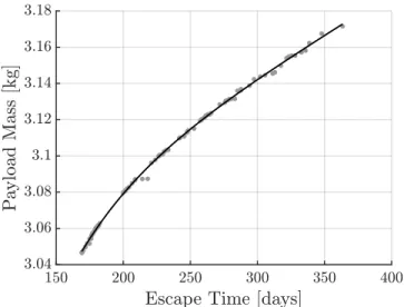
such that the spacecraft achieves escape. The Pareto front can be found with a genetic algorithm. Deb [17] provides a good reference on using genetic algorithms for multi-objective optimization. Figure 3-4 shows the resulting Pareto front for a minimum performance iEPS system on a 3U CubeSat starting from geostationary orbit. The points on the plot represent the result of the genetic algorithm while the black line is a second order exponential fit of the data. We can see that the tradeoff is quite poor - going from a 200 day trajectory to a 300 day trajectory only increases the payload mass by 60 grams meaning that we increase the payload mass by 0.6 grams per day that we sacrifice.

(59)

Figure 3-4: Pareto front for tradeoff in payload mass and escape time

points along the Pareto front can be simulated to see the trajectory. Figure 3-5 shows the trajectory, control thrust, and switching function for a 180 day escape trajectory along the Pareto front. Sections of the trajectory in black correspond to thruster firing while sections of the trajectory in red correspond to coasting. We can see based on the trajectory and control thrust that only a single coast arc is used. The time at which the thruster is turned off also corresponds to the time which the switching function is positive, as expected.

Figures 3-6 and 3-7 show Pareto dominant trajectories, control thrusts, and switch-ing functions for 205 and 365 day escape trajectories. We can see that as more and more coast arcs are added, the coast arcs are concentrated around where the orbital radius of the spacecraft is highest and therefore the orbital velocity is lowest - as expected. For the cases in Figures 3-5 and 3-6 we can see that the vast majority of thrusting is done during the initial spiral up from geostationary orbit with coast arcs being added to the final revolutions of the orbit. This helps to explain why the tradeoff between payload mass and escape time is so poor. During the initial spiral, the orbit of the spacecraft is very close to being circular and therefore there is no advantage to coasting. It’s only towards the end of the trajectory when the orbit be-comes slightly elliptical that the spacecraft can coast to take advantage of the Oberth effect and increase the payload mass.

(60)

Figure 3-5: Trajectory, control thrust, and switching function for a 180 day escape trajectory along the Pareto front

(61)

(62)

(63)

This effect can also be seen in Figure 3-7. Even though coast arcs are introduced lower in the trajectory, we can see that the orbits are still fairly circular. This means that the escape time is being significantly increased due to the added coasting but the payload mass is only marginally improved since the orbit is almost circular.

Based on this analysis and the analysis in Section 3.1.1 optimizations which aim to increase the payload mass delivered to escape do not provide significant results. Therefore, for these low-thrust escape trajectories the path forward is to use an angu-lar pointing control law, due to its simplicity, and continuous thrust with no coasting. Using such a control law dramatically decreases the complexity of designing escape trajectories. This allows us to develop good analytical approximations of the escape trajectory which can be used in analytical analyses of stage-based propulsion sys-tems as in Section 3.2.7 or as reference trajectories for guidance during circular orbit transfers or escape as in Section 4.2.

3.2 Analytical Analysis of Stage-Based Systems

To analyze the impact of using a stage-based propulsion system, an analytical ap-proach is taken. The analytical apap-proach allows us to view the dependencies of the stage-based propulsion system performance on the parameters of the individual stages. In addition, we can provide the framework to move towards autonomous decision mak-ing on satellites with stage-based propulsion systems by providmak-ing a computationally simple method for determining propulsion system performance.

The goal of the analytical approach is to develop equations that can answer key questions about the propulsion system. Namely,

• How many stages are required for a given mission?

• What are the dependencies on propulsion system parameters? • What is the mass and volume of the propulsion system? • How do un-staged and staged propulsion systems compare?

(64)

• What is the probability of mission success?

The answers to these questions all stem from an approximation of the ΔV of the propulsion system. We will find that we can provide a tight approximation of the true ΔV of the propulsion system both in cases where mass flow is neglected and where mass flow is accounted for. In addition, the approximation of ΔV will be conservative, meaning that any results derived from the approximation will bound the true result. These analytical approximations of the results can then be used in preliminary propulsion system and mission design, focusing of propulsion system technology developments, and online autonomous decision making.

3.2.1 ΔV Approximation

Ignoring fuel mass depletion, the ΔV for a stage-based propulsion system is given by ΔV = 𝑁 ∑︁ 𝑖=1 𝐹 𝐿 𝑚0− (𝑖 − 1)𝑚S (3.24) where 𝐹 is the propulsion system thrust, 𝐿 is the lifetime of each stage, 𝑚0 is the

initial spacecraft wet mass, and 𝑚S is the dry mass for a single stage. This sum does

not have an analytical solution. However, we can approximate its value by assuming that the impulse of each stage (𝐹 𝐿) is applied to the average mass of the spacecraft.

¯

𝑚 = 𝑚0−

1

2(𝑁 − 1)𝑚S (3.25)

This approximation eliminates the summing index from the sum itself and allows for a simple approximation of the ΔV for the whole system

ΔV ≈ 𝑁 ∑︁ 𝑖=1 𝐹 𝐿 𝑚0− 1₂(𝑁 − 1)𝑚S = 𝑁 𝐹 𝐿 𝑚0− 1₂(𝑁 − 1)𝑚S (3.26) Figure 3-8 shows the percent error in the ΔV approximation versus number of stages when compared to an exact calculation of the sum using minimum performance iEPS characteristics for a 3U CubeSat. We can see that the error is very small

Design and analysis of a stage-based electrospray propulsion system for CubeSats

Design and Analysis of a Stage-Based Electrospray

Propulsion System for CubeSats

by

Oliver Jia-Richards

S.B., Massachusetts Institute of Technology (2018)

Submitted to the Department of Aeronautics and Astronautics

in partial fulfillment of the requirements for the degree of

Master of Science in Aeronautics and Astronautics

at the

MASSACHUSETTS INSTITUTE OF TECHNOLOGY

June 2019

© Massachusetts Institute of Technology 2019. All rights reserved.

Author . . . .

Department of Aeronautics and Astronautics

May 20, 2019

Certified by. . . .

Paulo Lozano

M. Alemán-Velasco Professor of Aeronautics and Astronautics

Thesis Supervisor

Accepted by . . . .

Sertac Karaman

Associate Professor of Aeronautics and Astonautics

Chair, Graduate Program Committee

Design and Analysis of a Stage-Based Electrospray Propulsion

System for CubeSats

by

Oliver Jia-Richards

Abstract

Acknowledgments

Contents

List of Figures

List of Tables

Chapter 1

Introduction

1.1

Overview of Electrospray Propulsion

1.1.1

ion Electrospray Propulsion System

1.1.2

Lifetime Limitations of Electrospray Thrusters

1.2

Staging Concept

Chapter 2

Design

2.1

Staging Mechanism Design

2.1.1

Fuse Wire Material Selection

2.1.2

Vibration Analysis

2.2

Routing Mechanism Design

2.3

Stage Configuration

2.4

Mechanism Testing

2.4.1

Vacuum Testing

2.4.2

Fully Integrated Test

Chapter 3

Analysis

3.1

Un-staged Escape Trajectory

3.1.1

Comparison of Control Laws

3.1.2

Optimization with Calculus of Variations

3.2

Analytical Analysis of Stage-Based Systems

3.2.1

ΔV Approximation