HAL Id: inria-00143541
https://hal.inria.fr/inria-00143541v2
Submitted on 6 May 2008HAL is a multi-disciplinary open access
archive for the deposit and dissemination of sci-entific research documents, whether they are pub-lished or not. The documents may come from teaching and research institutions in France or
L’archive ouverte pluridisciplinaire HAL, est destinée au dépôt et à la diffusion de documents scientifiques de niveau recherche, publiés ou non, émanant des établissements d’enseignement et de recherche français ou étrangers, des laboratoires
Estimation of the Brownian dimension of a continuous
Ito process
Jean Jacod, Antoine Lejay, Denis Talay
To cite this version:
Jean Jacod, Antoine Lejay, Denis Talay. Estimation of the Brownian dimension of a continuous Ito process. Bernoulli, Bernoulli Society for Mathematical Statistics and Probability, 2008, 14 (2), pp.469-498. �10.3150/07-BEJ6190�. �inria-00143541v2�
Estimation of the Brownian dimension
of a continuous Itˆo process
Jean Jacod
Institut de Math´ematiques de Jussieu
Universit´e Pierre et Marie Curie et CNRS (UMR 7586) 4 Place Jussieu
75252 PARIS Cedex 05 France
Antoine Lejay INRIA Nancy – Grand Est IECN, Campus Scientifique
B.P. 239
54506 Vandœuvre-l`es-Nancy Cedex France
Denis Talay
INRIA Sophia Antipolis – M´editerran´ee 2004 Route des Lucioles
B.P. 93
06902 Sophia-Antipolis France
Summary. In this paper we consider a d-dimensional continuous Itˆo process, which is observed at n regularly spaced times on a given time interval [0, T ]. This process is driven by a multidimensional Wiener process, and our aim is to provide asymptotic statistical procedures which give the minimal dimension of the driving Wiener process, which is between 0 (a pure drift) and d. We exhibit several different procedures, which are all similar to asymptotic testing hypotheses.
Keywords. Asymptotic testing, Brownian dimension, Discrete observations, Itˆo pro-cesses.
Running title. Estimation of the Brownian dimension
This article has been published in Bernoulli
hhttp://isi.cbs.nl/bernoulli/i, 14:2, 469–498 (2008)
1
Introduction
In numerous applications, one chooses to model a complex dynamical phenomenon by stochastic differential equations or, more generally, by semimartingales, either because random forces excite a mechanical system, or because time–dependent uncertainties dis-turb a deterministic trend, or because one aims to reduce the dimension of a large scale system by considering that some components contribute stochastically to the evolution of the system. Examples of applications respectively concern mechanical oscillators submit-ted to random loading, prices of financial assets, molecular dynamics.
Of course the calibration of the model is a crucial issue. A huge literature deals with the statistics of stochastic processes, particularly of diffusion processes: Parametric and non-parametric estimators of the coefficients of stochastic differential equations have been intensively studied; see for example the books [6] and [7] of Prakasa Rao, in which a large number of papers are quoted and analyzed. However, somewhat astonishingly, it seems to us that most of the papers consider that the dimension of the noise is known by the observer. This hypothesis is often questionable: there is no reason to a priori fix this dimension when one observes a basket of assets, or a complex mechanical structure in a random environment. Actually the last two authors of this paper were motivated to study this question by modelling and simulation issues related to the pricing of contracts based on baskets of energy prices (see O. Bardou’s thesis [3]). There was no determining financial reason to fix the Brownian motion dimension to a particular value. In addition, the interest to find an as small dimension as possible was two-fold: first, one then avoids the calibration of useless diffusion matrix components; second, practitioners need that the simulation of the model, and thus the computation of contract prices and of corresponding risk measures by means of Monte Carlo simulations, are as quick as possible.
We thus try, in this paper, to tackle the question of estimating the Brownian dimension of an Itˆo process from the observation of one trajectory during a finite time interval. More precisely, we aim to build estimators which provide an “explicative Brownian dimension”
rB: a model driven by a rB Brownian motion satisfyingly fits the information conveyed
by the observed path, whereas increasing the Brownian dimension does not allow to fit the data any better. Stated this way, the problem is obviously ill posed, hence our first step consists in defining a reasonable framework to develop our study.
Suppose that we observe a continuous d–dimensional Brownian semimartingale X = (Xi)
1≤i≤d on some space (Ω, F, (Ft), P). The observation time interval is [0, T ] with T
finite. The process X is a continuous Itˆo process, meaning that it satisfies the following assumption: Hypothesis (H): We have Xt= X0+ Z t 0 asds + Z t 0 σs dWs, (1)
where W is a standard q–dimensional BM, a is a predictable Rd–valued locally bounded
process, and σ is a d × q matrix–valued adapted and c`adl`ag processes (in (1) one can replace σs by the left limit σs−, so as to have a predictable integrand, if one wishes).
We say that we are in the “pure diffusion case” when σs= σ(Xs). We set cs = σsσs?
(so cs = c(Xs) where c = σσ? in the pure diffusion case). The process c takes its values in
the set Md of all d × d symmetric nonnegative matrices. We denote by rank(Σ) the rank of any Σ ∈ Md.
As it is well known, the same process X can be written as (1) with many different Wiener processes; namely if (Πs) is a progressively measurable process taking its values
in the set of q × q orthogonal matrices, then W0 t =
Rt
0ΠsdWs is another q-dimensional Wiener process and X is of the form (1) with W0 and σ0
s= σsΠ−1s . Then the “Brownian
dimension” rBof our model is defined as being the smallest integer r such that, after such
a transformation, the last q − r columns of σ0
s(ω) vanish (outside a P(dω)ds-null set, and
for s ≤ T of course). In this case, we can forget about the last q − r components of W0
and in fact write (1) with an r-dimensional Wiener process. Obviously rB≤ d always, so
one could start with a model (1) with q ≤ d always, but it is convenient for the discussion in this paper to take q arbitrary.
Our aim is to make some kind of inference on this Brownian dimension rB, which is
also the maximal rank of cs (up to a P(dω)ds-null set), on the basis of the observation of the variables XiT /n for i = 0, 1, . . . , n, where [0, T ] is the time interval on which the process is available. Let us make some preliminary comments, in which we refer to the “ideal” and “actual” observation schemes when one observes X completely over [0, T ], or at times iT /n only, respectively.
1) Suppose we are in the pure diffusion case, that is cs = c(Xs) with c a continuous function, and that the range of the process is the whole of Rd (that is, every open
subset of Rd is visited by X on the time interval [0, T ] with a positive probability).
Set r(x) := rank(c(x)), and let A(ω) be the subset of Rdwhich is visited by the path
(X(ω)t: t ∈ [0, T ]). The Brownian dimension is rB= supx∈Rdr(x), but in the ideal
scheme we observe R(ω) = supx∈A(ω)r(x) and so we can only assert that r ≥ R(ω).
The situation is similar to what happens in the non-parametric estimation of the function c : in the ideal scheme this function c is known on A(ω) and hopelessly unknown on Rd\A(ω).
2) More generally, the only relevant quantity we might hope to “estimate” is the (ran-dom) maximal rank
R(ω) = sup
s∈[0,T )
rank(cs(ω)) (2)
(we should take the essential supremum rather than the supremum, but the two agree since cs is right-continuous in s). The variable R is integer–valued, so its “estimation” is more akin to testing that R = r for any particular r ∈ {0, . . . , d}, although it will not be a test in the ordinary sense because R is random. Note that in many models we will have that rank(cs(ω)) is independent of s and ω; then R is
non–random, but this property does not really makes the analysis any easier.
3) In the actual scheme we will construct an integer–valued statisticsRbnwhich serves as an “estimator” for R. We have to somehow maximize (and evaluate) the probability that Rbn = R, or perhaps this probability conditional on the value taken by R,
or conditional on the whole path of X over [0, T ]. That is, we perform a kind of “conditional test”.
4) We might also take a different look at the problem. Considering the model (1), we can introduce a kind of “distance” ∆r between the true process X and the class
of all processes X0 of the same form, but with a diffusion coefficient c0
s satisfying
identically rank(c0
s) ≤ r. Then we construct estimators ∆nr for ∆r, for all values of
r, and decide on the basis of these ∆n
r which Brownian dimension rB is reasonable
to consider for the model. The mathematical problem is then similar to the semi– parametric estimation of a parameter in the diffusion coefficient for a discretely observed diffusion with unknown drift: here the “parameter” is the collection of all ∆r, and the unknown (nuisance) parameters are the processes as and cs (or σs).
The paper is organized as follows: In Section 2 we explain in a more precise way the “distances” mentioned above. Section 3 is a collection of simple linear algebra results, and Section 4 contains the basic limiting results needed. Then in Sections 5 and 6 we put the previous results in use to develop some statistical applications, and finally we provide some numerical experiments in Section 7.
2
An instructive but non effective approach
In this section we measure the discrepancy between the model (1), and models of the same type but with a different Brownian dimension. We denote by Sr the set of all c`adl`ag
adapted d × q matrix–valued processes σ0 such that c0
s = σ0sσ0?s satisfies rank(c0s) ≤ r a.s.
for all s. In particular S0 contains only σ0≡ 0. With any σ0 ∈ Sr we associate the process
Xt0 = X0+ Z t 0 asds + Z t 0 σ 0 s dWs, (3)
with the same a and the same W than in (1).
A measure of the “distance” between the two processes X and X0 of (1) and (3),
measured on the time interval [0, t], is the random variable ∆(X, X0)
t defined below: in
the next formula H ranges through all predictable d-dimensional process with kHt(ω)k ≤ 1 for all (ω, t) and H? is the transpose; hM i is the quadratic variation process of the
semimartigale M and • denotes stochastic integration: ∆(X, X0)t= sup
H :kHk≤1
hH?• (X − X0)it. (4)
This measurement of the discrepancy between X and X0 is particularly well suited to
finance, where E(∆(X, X0)
t) is a measure of the difference in the L2 sense between the
portfolio evaluations when one takes the model with X or the model with X0. Then set ∆(r; X)t= inf(∆(X, X0)t: X0 is given by (3), with σ0 ∈ Sr) (5)
for the “distance” from X to the set of semimartingales with Brownian dimension not more than r, again on the time interval [0, t].
Remark 1 Of course ∆(X, X0)
t is not a genuine distance, for two reasons: it does not
satisfy the triangle inequality (it is rather the square of a distance), and more impor-tant it is random. The genuine distance (which is one of Emery’s distances, see [5]) is
p
E(∆(X, X0)t), provided we identify two processes which are a.s. equal, as usual.
Also, note that the two approaches, here where W is kept fixed, and in the previous section where W may be changed into another Wiener process W0, look different but are
actually the same. 2
The next proposition shows how to compute “explicitly” ∆(r; X)t. We denote by
λ(1)s≥ λ(2)s≥ . . . ≥ λ(d)s≥ 0 the eigenvalues of the matrix cs, and we set
L(r)t= Z t
0 λ(r)s ds. (6)
Proposition 2 For any r = 0, . . . , d − 1 we have ∆(r; X)t= L(r + 1)t, and the infimum
in (5) is attained.
Proof. It is no restriction to suppose that q ≥ d (if not, we can always add independent components to W , and accordingly components to σ which are 0). Let J be the d × q matrix with (i, i) entry equal to 1 when 1 ≤ i ≤ d, and all other entries equal to 0. Then we can find two c`adl`ag adapted processes Πs and Qs, with values in the sets of d × d and
q × q orthogonal matrices respectively, and such that σs = ΠsΛ1/2s JQs, where Λs is the
diagonal matrix with entries λ(i)s. Note that cs= ΠsΛsΠ?s.
Let Ir (resp. I0
r) be the d × d matrix with (i, i) entry equal to 1 when 1 ≤ i ≤ r (resp.
r + 1 ≤ i ≤ d), and all other entries equal to 0. Then we set σ0s = ΠsΛ1/2s IrJQs and we
associate X0 by (3). Then σ s− σs0 = ΠsΛ1/2s Ir0JQs, and thus hH?• (X − X0)it= Z t 0 (H ? sΠsΛ1/2s Ir0JQsQ?sJ?Ir0Λ1/2s Π?sHs)ds.
The integrand above is simply Hs?ΠsΛ1/2s Ir0Λ1/2s Π?sHs and, if kHsk = 1, we also have
kΠ?
sHsk = 1 and thus this integrand is not bigger than λ(r + 1)s: therefore ∆(X, X0)t≤
L(r + 1)t. Furthermore σ0sσ0?s = ΠsΛsIrΠ?s is of rank ≤ r, so σ0 ∈ Sr.
Now, let σ0 be any process in S
r and put c0s = σs0σs0?. The kernel Ks0 of the linear
map on Rd associated with the matrix c0
s is of dimension at least d − r. The subspace
Ks of Rd generated by all eigenvectors of this linear map, which are associated with the
eigenvalues λ(1)s, . . . , λ(r + 1)s, is of dimension at least r + 1 (it is strictly bigger than
r + 1 if λ(r + 1)s= λ(r + 2)s). Then Ks∩ Ks0 is not reduced to {0}, and we thus can find
a process H = (Hs)s≥0 with kHsk = 1 and Hs ∈ Ks∩ K0
s identically, and obviously this
process can be chosen to be progressively measurable. Then c0
sHs= 0 (because Hs∈ Ks0)
and H?
scsHs ≥ λ(r + 1)skHsk = λ(r + 1)s (because Hs ∈ Ks). The first property above
yields H?• Xt0 = Z t 0 H ? sasds, hence hH?• (X − X0)it= hH?• Xit= Z t 0 (H ? sc?sHs)ds,
which by the second property above is not less than L(r + 1)t: hence we are done. 2
In particular, L(1)t= ∆(0; X)tmeasures the “distance” between the process X and the
pure drift process X0+
Rt
0asds. The following is obvious, with the convention L(d+1)t= 0 :
Rt≤ r ⇐⇒ L(r + 1)t= ∆(r; X)t= 0, (7)
where, similar to (2), we have set for all t > 0:
R(ω)t= sup s∈[0,t]
rank(cs(ω)). (8)
Hence the random value L(r + 1)t measures the distance between X and the set of all
processes with Brownian dimension r, over the time interval [0, t], and for our particular
path of X. Note also that it is an “absolute” measure of the distance, which is multiplied
by u2 if we multiply the process X by u.
Unfortunately, the variables L(r)t do not seem to be easy to “estimate” from discrete observations since they involve eigenvalues. Hence we will construct below estimators which are easier to handle.
3
Linear algebra preliminaries
Consider for a moment the toy model X = σW , where σ is a non-random d × q matrix. That is, we have (1) with X0 = 0 and as = 0 and σs(ω) = σ, or equivalently X is a
Wiener process with covariance Σt at time t, where Σ = σσ?. The observation scheme
amounts to observing n i.i.d. random vectors Gi, all of them N (0, Σ)–distributed (namely
Gi = p
n/T ∆niX, with the notation ∆niX = XiT /n− X(i−1)T /n). To infer rank(Σ) from the observations of the n first variables Gk, we can use the empirical covariance
b Σn= 1 n n X k=1 GkG?k. (9)
Indeed, the variables Gkhave a density over their support, which is a linear subspace with
dimension rank(Σ): hence rank(Σbn) is almost surely equal to n when n < rank(Σ), and
to rank(Σ) otherwise, and the problem is solved in a trivial way.
If we are in the same setting, except that cs depends on s (and is still deterministic)
and has a constant rank r, then typically the eigenspaces “rotate” when s varies, and the rank of Σbn above is a.s. equal to d as soon as n ≥ d. Therefore Σbn gives no insight on
the rank. So the problem for nonhomogeneous Wiener process, and a fortiori for general diffusions like (1), is actually more complex.
Despite the uselessness of the toy model consisting of an homogeneous Wiener process, let us give a couple of formulas about it, for further reference. We denote by Arthe family
of all subsets of {1, . . . , d} with r elements (r = 1, . . . , d). If K ∈ Ar and Σ = (Σij) ∈ Md
we denote by detK(Σ) the determinant of the r × r sub–matrix (Σkl : k, l ∈ K), and we
set
det(r; Σ) = X
K∈Ar
Observe that det(d; Σ) = det(Σ), while det(1; Σ) is the trace of Σ.
Lemma 3 If Σ ∈ Md has eigenvalues λ(1) ≥ . . . λ(d) ≥ 0, we have for r = 1, . . . , d:
1
d(d − 1) . . . (d − r + 1) det(r; Σ) ≤ λ(1)λ(2) . . . λ(r) ≤ det(r; Σ). (11)
Notice that both inequalities in (11) may be equalities. It follows from (11) that, with the convention 0/0 = 0, we have
1 ≤ r ≤ d =⇒ r ≤ rank(Σ) =⇒ det(r; Σ) > 0 r > rank(Σ) =⇒ det(r; Σ) = 0, (12) 2 ≤ r ≤ d =⇒ r! d! det(r; Σ) det(r − 1; Σ) ≤ λ(r) ≤ d! (r − 1)! det(r; Σ) det(r − 1; Σ). (13)
Proof. We expand the characteristic polynomial of Σ as
det(Σ − λI) = (−λ)d+
d X r=1
(−λ)d−rdet(r; Σ).
In view of the well known expressions for the “symmetrical functions” of the roots of a polynomial, we get
X
1≤i1<...<ir≤d
λ(i1)λ(i2) . . . λ(ir) = det(r; Σ),
and thus both sides of (11) are obvious. 2
Next, we consider a sequence (Gi)i≥1of i.i.d. N (0, Σ)-distributed random vectors. For
all j = 1, . . . , d we define two random elements of Mdby
ζj = j X i=1 GiG?i, ζj0 = d+j X i=d+1 GiG?i, (14)
and we consider the mean and covariance of the random vector (det(r; ζr)/r! : 1 ≤ r ≤ d):
γ(r; Σ) = 1 r! E(det(r; ζr)), Γ(r, r0; Σ) = 1 r!r0! E(det(r; ζr) det(r0; ζr0)) − γ(r; Σ)γ(r0; Σ). ) (15)
Since (ζj, ζj0 : 1 ≤ j ≤ d) are i.i.d. we also have
Γ(r, r0; Σ) = 1
r!r0! E ³
det(r; ζr) det(r0; ζr0) − det(r; ζr) det(r0; ζr00)
´
Lemma 4 If r ∈ {1, . . . , d}, we have γ(r; Σ) = det(r; Σ). (17) Moreover r ≤ rank(Σ) ⇒ γ(r; Σ) > 0, Γ(r, r; Σ) > 0 r > rank(Σ) ⇒ γ(r; Σ) = 0, Γ(r, r; Σ) = 0. (18)
Proof. For proving (17) it is enough to show that for any K ∈ Ar, we have E(detK(ζr)) =
r! detK(Σ), and for this it is no restriction to assume that K = {1, . . . , r}. We denote
by Pr the set of all permutations of the set {1, . . . , r}, and ε(τ ) is the signature of the
permutation τ . Then detK(ζr) = X τ ∈Pr (−1)ε(τ ) r Y l=1 ζrlτ (l)= X 1≤k1,...,kr≤r X τ ∈Pr (−1)ε(τ ) r Y l=1 Glkl Gτ (l)kl ,
and each summand of the first sum of the extreme right side is the determinant of a matrix with rank less than r, unless all kl are distinct. So it is enough to sum over all r–uples (k1, . . . , kr) with distinct entries between 1 and r, that is for r–uples with ki = τ0(i) for
some τ0 ∈ P
r. In other words, we have
detK(ζr) = X τ0∈Pr X τ ∈Pr (−1)ε(τ ) r Y l=1 Glτ0(l) Gτ (l)τ0(l). (19)
Since the variables Gn are independent and E(GknGln) = Σkl, we deduce that
E(detK(ζr)) = r! X τ ∈Pr (−1)ε(τ ) r Y l=1 Σlτ (l)= r! detK(Σ), and we have (17).
If r > rank(Σ) we have det(r; Σ) = 0 (see (12)): the nonnegative variable det(r; ζr)
has zero expectation, so it is a.s. null, and we have the second part of (18). Finally let
r ≤ rank(Σ). By (12) again we have E(det(r; ζr)) > 0. Also, observe that det(r; ζr) is a continuous function of the random vectors Gn for n = 1 . . . , r, which vanishes if all these
Gnare 0. Thus det(r; ζr) can take arbitrarily small values with a positive probability, and
it has a positive expectation, so it is not degenerate and we get the first part of (18). 2
4
Limit theorems for estimators of the Brownian dimension
It turns out that determinants or “integrated determinants”, are much easier to estimate than eigenvalues or integrated eigenvalues. So in view of (11) and (12) one might replace the variable L(r)tof (6) by L0(r)t= Rt 0det(1; cs) ds if r = 1 Rt 0 detdet(r−1;c(r;cs)s) ds if r ≥ 2.However, L0(r)
t for r ≥ 2 is still not so easy to estimate: for example for the toy model
of Section 3 the variable det(r; ζr)/r! is an unbiased estimator of det(r; Σ) (see (17)), but
we have no explicit unbiased estimator for a quotient like det(r; Σ)/ det(r − 1; Σ). So we propose to measure the distance between X and the set of models with multiplicity
r, over the time interval [0, t], by the following random variable: L(r)t=
Z t
0 det(r; cs) ds. (20)
Up to multiplicative constants, this more or less amounts to replace the “natural” distance
L(r)t by Rt
0λ(1)s. . . λ(r)s ds. The variables L(r)t, L0(r)t and L(r)t convey essentially the same information as far as rank is concerned, and in particular they vanish simultaneously, which is the most important property for our purposes. In other words, exactly as in (7) we have
Rt≤ r ⇐⇒ L(r + 1)t= 0, (21)
By virtue of (17) we can rewrite L(r) as follows (we also introduce additional variables
Z(r, r0), using the notation (15)):
L(r)t= Z t 0 γ(r; cs) ds, Z(r, r 0) t= Z t 0 Γ(r, r 0; c s) ds. (22)
Now, we need to approximate the variables in (22) by variables which depend on our discrete observations only. To this end we introduce the random matrices
ζ(r)ni =
r X j=1
(∆ni+j−1X) (∆ni+j−1X)?, where ∆n
iX = XiT /n− X(i−1)T /n. (23)
We have ζ(r)n
i ∈ Md and rank(ζ(r)ni) ≤ r. Then we set (with [x] being the integer part
of x): L(r)nt = nr−1 Tr−1 r! [nt/T ]−r+1X i=1 det(r; ζ(r)ni), (24) and Z(r, r0)nt = nr+r 0−1 Tr+r0−1 r! r0! [nt/T ]−d−r0+1 X i=1 ³ det(r; ζ(r)ni) det(r0; ζ(r0)ni)
−det(r; ζ(r)ni) det(r0; ζ(r0)nd+i)´. (25)
The first key theorem is the “consistency” of these variables:
Theorem 5 Under (H) the variables L(r)n
t and Z(r, r0)nt converge in probability to L(r)t
and Z(r, r0)
t respectively, uniformly in t ∈ [0, T ].
This is not enough for our purposes, and we need rates of convergence. For this (H) is not sufficient, and some additional regularity on the coefficients a and σ is necessary. A first set of sufficient conditions is simple enough:
Hypothesis (H1): We have (H) with a c`adl`ag process a, and a process σ which is H¨older continuous (in time) with index ρ > 1/2, in the sense that
sup 0≤s<t≤T
kσt− σsk
(t − s)ρ < ∞ a.s. (26)
The assumption on a above is quite mild, and the assumption on σ is reasonable when
σ is deterministic. However, in the pure diffusion case we have σs = σ(Xs) for, say, a
Lipschitz or locally Lipschitz function σ, and of course (26) fails for any ρ ≥ 1/2. This assumption also fails when σs is a “stochastic volatility” driven by an Itˆo equation, and
even more if this equation has jumps !
Therefore, for practical purposes which are especially relevant in finance, we need to replace (H1) by a different assumption. This assumption looks (is ?) complicated to state, but it essentially says that a is as in (H1), and that the process σ follows a jump-diffusion Itˆo equation, or in other words that it is driven by a Wiener process and a Poisson random measure); in particular it is satisfied in the pure diffusion case when σs = σ(Xs) with a
C2 function σ.
Hypothesis (H2): We have (H), the process a is c`adl`ag, and the process σ is a (possibly discontinuous) Itˆo semimartingale on [0, T ], that is for t ≤ T we have
σt = σ0+ Z t 0 a 0 sds + Z t 0 σ 0 s−dWs + Z t 0 Z Eϕ ◦ w(s−, x)(µ − ν)(ds, dx) + Z t 0 Z E(w − ϕ ◦ w)(s−, x)µ(ds, dx). (27)
Here σ0 is Rd⊗ Rq⊗ Rq-valued adapted c`adl`ag, and a0 is Rd⊗ Rq–valued predictable
and locally bounded; µ is a Poisson random measure on (0, ∞) × E independent of W and V , with intensity measure ν(dt, dx) = dtF (dx) with F a σ–finite measure on some Polish space (E, E); ϕ is a continuous function on Rdq with compact support, which
coincides with the identity on a neighborhood of 0); finally w(ω, s, x) is a map Ω×[0, ∞)×
E → Rd⊗ Rq which is Fs⊗ E–measurable in (ω, x) for all s and c`adl`ag in s, and such
that RE(1Vsupω∈Ω,s≤Tkw(ω, s, x)k2) F (dx) < ∞.
These conditions are indeed quite easy to check in practice. They accommodate the case of a stochastic volatility driven by a Wiener process having some (or all) components independent of X: since W has an “arbitrary” dimension q in this paper, possibly q > d, there might be components used for X in (1) and other components used in (27).
Theorem 6 Assume either (H1) or (H2). The d–dimensional processes (V (r)n t)1≤r≤d with components
V (r)nt =√n (L(r)nt − L(r)t) (28)
converge stably in law to a limiting process (V (r)t)1≤r≤d, which is defined on an extension of the original space and which, conditionally on F, is a non-homogeneous Wiener process with quadratic variation process t 7→ (T Z(r, r0)
Proof of Theorems 5 and 6. The proof goes through several steps:
1) It is based on the following two results of [4]. Take N functions gj on Rd, which are
C2 and with polynomial growth and even. Set
Y (g1, . . . , gN)nt = T n [nt/T ]−N +1X i=1 N Y k=1 gk( q n/T ∆ni+k−1X).
Then under (H) we have
Y (g1, . . . , gN)nt −→ Y (gP 1, . . . , gN)t:= Z t
0 y(g1, . . . , gN; cs) ds,
where the convergence in uniform in t ∈ [0, T ] and where y(g1, . . . , gN; Σ) is, for any d × d covariance matrix Σ, the expectation of the variable
γ(g1, . . . , gN) =
N Y k=1
gk(Gk)
and the Gn’s are i.i.d. random vectors with law N (0, Σ), as in Section 3.
If further (H2) holds, then for any array³(g1j, . . . , gjNj) : 1 ≤ j ≤ J´ with gji as above, the J–dimensional processes ³pn/T (Y (gj1, . . . , gNjj)n
t − Y (g1j, . . . , gNjj)t
´
1≤j≤J converge stably in law to a limiting process which, conditionally on F, is a non-homogeneous Wiener process with quadratic variation process R0tΓ(cs)ds, and where Γ(Σ) is the covariance
matrix of the random vector ³γ(g1j, . . . , gNjj)´
1≤j≤J as defined above. Under (H1) instead of (H2) the same result holds: it is not explicitely stated in [4], but the proof is similar and technically much simpler.
2) These results extend by ”linearity” in an obvious way. More precisely, for 1 ≤ j ≤ J set Y (j)nt = T n [nt/T ]−NXj+1 i=1 hj µq n/T ∆n iX, q n/T ∆ni+1X, . . . , q n/T ∆ni+Nj−1X ¶ , (29)
where each hj is a linear combinations of tensor products g1⊗ . . . ⊗ gNj, where the gi’s
are C2 functions on Rd, even and with polynomial growth. Let also denote by M (Σ)
and C(Σ) the mean vector and the covariance matrix of the J–dimensional random vector (hj(G1, . . . , GNj)1≤j≤J, with Gi as above. Then:
1. under (H) we have Y (j)nt −→ Y (j)P t:= Z t 0 M j(c s)ds, uniformly in t ∈ [0, T ]; (30)
2. under (H1) or (H2) the J-dimensional processes with components pn/T (Y (j)n t −
Y (j)t) converge stably in law to a limiting process which, conditionally on F, is a
3) The theorem is now almost trivial. The determinants entering (24) and (25) are sums of even monomials of the components of ∆n
i+j−1X for 1 ≤ j ≤ 2d, each one with degree
2r, resp. 2(r + r0). More specifically, L(r)n is of type (29), with Nr = r and the function
hr(x1, · · · , xr) = r!1 det ³ r, r X j=1 xjx?j ´ ,
whereas Z(r, r0)nis of type (29), with Nr,r0 = d + r0 and the function
hr,r0(x1, · · · , xd+r0) = 1 r! r0! det³r,Xr j=1 xjx?j ´ det³r0, r0 X j=1 xjx?j ´ − det³r, r X j=1 xjx?j ´ det³r0, d+r0 X j=d+1 xjx?j ´ .
Then Theorem 5 readily follows from Step 2 and from the relations (15). 2
In the sequel we will need also some estimates on the moments of V (r)n
t, uniform in
n. It follows from the proofs in [4] that, under (H2) and for each t ∈ (0, T ], there is a
sequence Ap,t of Ft–measurable sets such that
Ap,t↑ Ω as p → ∞
p ≥ 1, n ≥ 1, t ∈ (0, T ] =⇒ E(|V (r)n
t|21Ap,t) ≤ Cp,
)
(31)
for a suitable sequence of constants Cp (depending on T ). This very same result also holds
under (H1).
Now, if the coefficient a is bounded, and if we have (H1) with (26) holding uniformly in ω, or (H2) with a0
s(ω) and σs0 − ω) bounded and kw(ω, s, x)k ≤ h(x) for some function
having RE(1Vh(x)2)F (dx) < ∞, one can (easily) prove that (31) holds for A
1,t= Ω, and so there is a constant C, depending on T , such that
n ≥ 1, t ∈ (0, T ] =⇒ E(|V (r)nt|2) ≤ C. (32)
5
Tests based on thresholds
5.1 A test based on an absolute threshold
We come back to the initial problem, in the light of the second comment of Section 1: namely, we want to decide which integer value (between 0 and d) the variable R of (2) takes for the particular path ω which is known only through the observations XiT /n. In principle we have our observations XiT /n for i = 0, . . . , n, but it may be interesting to determine how our estimators behave as time changes; this is why we also give estimators for the variable Rt of (8), based on the observation of XiT /n for i = 0, . . . , [nt/T ].
Let us say once more that in the ideal scheme (the whole path of X is known over [0, T ]) we also know R = R(ω), whereas we have the equivalence (21). In view of this, and
taking into account the convergence result in Theorem 5, it seems natural to operate as follows: we choose a sequence of positive numbers ρn such that
ρn→ 0, ρn
√
n → ∞. (33)
Then we take the following ”estimator” for Rt:
b
Rn,t= inf³r ∈ {0, . . . , d − 1} : L(r + 1)nt < ρnt´, (34)
with inf(∅) = d. That this estimator is a priori reasonable comes from the fact that if we set Rn,t = inf³r ∈ {0, . . . , d − 1} : L(r + 1)t< ρnt´, then by (21) and the property
ρn → 0, we have P(Rn,t = Rt) → 1 as n → ∞. We take a threshold of the form ρnt
because L(r + 1)n
t is roughly proportional to t.
Remark 7 Another equally reasonable estimator, which is a kind of “dual” ofRbn,t, is the
following one:
b
R0n,t= sup³r ∈ {1, . . . , d} : L(r)nt ≥ ρnt´, (35)
with sup(∅) = 0. The analysis ofRbn,t made below carries over forRb0n,t in pretty much the
same way. 2
Remark 8 The choice of the threshold ρn is arbitrary, upon the fact that (33) holds: asymptotically all choices are equivalent. In practice, though, it is of primary importance because n, albeit large, is given and is of course not infinite ! Even worse, an absolute threshold like in (34) is sensitive to the unit in which the values of the Xi
t are expressed:
for example if we multiply all components by the same (known) constant the estimator of the Brownian dimension provides a different value. So using an absolute threshold is probably not advisable in general. Nevertheless we pursue here the analysis of tests based on an absolute threshold, since they may serve as a case study and are somewhat simpler to study than the tests based on relative thresholds which are introduced later. 2
The integer–valued estimator Rbn,t should be analyzed using the testing methodology
rather than as a usual estimator: we test the hypothesis Rt = r with the critical region
{Rbn,t6= r}. The “power function” is in principle the probability of rejection, a function of
the underlying probability measure. Here we have a single P, and Rtis (possibly) random.
We thus develop two different substitutes to the power function.
5.2 A first substitute to the power function
A seemingly acceptable version of the power function is
b
βn,tr (r0) = P(Rbn,t6= r | Rt= r0), r0 = 0, 1, . . . , d, (36)
provided P(Rt = r0) > 0. We explicitly mention the number n of observations and the
number r, but it also depends on the sequence ρn. The index r indicates the “test” with null hypothesis Rt = r which we are performing, while the index r0 indicates the “true”
value or Rt: so βbn,tr (r) should be small, andβbn,tr (r0) should be close to 1 when r0 6= r.
Theorem 9 Under (33) and either (H1) or (H2) we have for all r, r0 in {1, . . . , d}, and provided P(Rt= r0) > 0: b βn,tr (r0) −→ ( 1 if r 6= r0 0 if r = r0. (37)
Another equivalent (simpler) way of stating this result consists in writing
P(Rbn,t6= Rt) → 0. (38)
This is more intuitive, but somehow farther away from the way results on tests are usually stated.
Proof. For each s = 1, . . . , (r0+ 1) ∧ d we set δn,ts (r0) = P(L(s)nt < ρn, Rt= r0). Observe
that, if ρ0 n= ρn
√
n, and with the notation (28), δs n,t(r0) ≤ P(L(s)t< 2ρnt, Rt= r0) + P(|V (s)nt| > ρ0nt), P(Rt= r0) − δn,ts (r0) ≤ P(L(s)t> ρnt/2, Rt= r0) + P(|V (s)nt| ≥ ρ0nt/2). (39)
Theorem 6 yields that the sequence V (s)n
t converges in law when n goes to infinity, whereas
on the set {Rt = r0} we have L(s)
t > 0 if s ≤ r0, and L(s)t = 0 if s > r0. Therefore it
follows from (33) that
s ≤ r0 ⇒ δs n,t(r0) → 0 s = r0+ 1 ≤ d ⇒ δs n,t(r0) → P(Rt= r0). ) (40)
Now {Rbn,t6= r0} = (∪1≤s≤r0{L(s)tn< ρnt}) ∪ {L(r0+ 1)nt ≥ ρnt}, with the convention
{L(d + 1)n t ≥ ρnt} = ∅. Then P(Rbn,t6= r0= Rt) ≤ Pr0 s=1δsn,t(r0) + P(Rt= r0) − δr 0+1 n,t (r0) if r0≤ d − 1 Pr0 s=1δsn,t(r0) if r0= d.
Then it readily follows from (40) that βbr0
n,t(r0) → 0 as soon as P(Rt= r0) > 0. Under this
assumption and if r 6= r0 we clearly haveβbr
n,t(r0) = 1 − P(Rbn,t= r | Rt= r0) ≥ 1 −βbr
0
n,t(r),
hence βbr
n,t(r0) → 1. 2
The previous result seems to settle the matter. However, it is not as nice as it may look, because it gives no “rate” for the convergence in (37) or (38) and is thus impossible to put in use in practice. The impossibility of getting a rate is apparent in (39): the second terms on the right may be more or less controlled through estimates like (31), but the first terms on the right cannot be controlled at all; indeed if Rt= r the variable L(r)t
5.3 A second substitute to the power function
As emphasized in Comment 4 of Section 1, one may reasonably decide that Rt= r if r is
the “true” Brownian dimension in a “significant” way, which means in particular that the “distance” between the model X and the set of models with Brownian dimension r0 < r
is not “infinitesimal”. This may be interpreted as the property that L(r)t exceeds some
positive level for all r ≤ Rt.
In other words, we set Br0,ε,t = {Rt = r0, L(r)t ≥ εt for r = 1, . . . , r0}, and we define
the “power function” as being
b
βn,tr (r0, ε) = P(Rbn,t6= r | Br0,ε,t), (41)
provided P(Br0,ε,t) > 0.
Evaluating βrn,t(r0, ε) is still difficult, because it involves the unknown quantity P(Br0,ε,t).
So we provide a result which does not directly give the power function itself, but which is probably more relevant for applications.
Theorem 10 Under (H1) or (H2) there are Ft-measurable sets (Ap,t) increasing to Ω as
p → ∞, and constants Cp such that, for all r in {1, . . . , d}, and provided ρn< ε/2:
P({Rbn,t6= r} ∩ Br,ε,t∩ Ap,t) ≤ nρCp2 n
(42)
for all t ∈ (0, T ]. If further (32) holds, we can find a constant such that
P({Rbn,t6= r} ∩ Br,ε,t) ≤ nρC2 n
, (43)
or in other words, the “level” satisfies βbr
n,t(r, ε) ≤ C/ ³ nρ2 nP(Br,ε,t) ´ .
Note that we can choose ρn above at will, provided it satisfies (33), and neither Apnor
Br0,ε,t nor Cp depend on this choice (the estimator Rbn,t does, though): so we can obtain
a rate 1/nθ for any θ ∈ (0, 1), as close to 1 as one wishes.
Proof. We consider the sets Ap,tfor which (31) holds, and we denote by Cp0 the constants
occurring in that formula. For s = 1, . . . , (r + 1) ∧ d we set (ε > 0 being fixed) δs
n,t(r, p) =
P({L(s)n
t < ρnt} ∩ Br,ε,t∩ Ap,t). Exactly as for (39), we have
δn,ts (r, p) ≤ P({L(s)t< 2ρnt} ∩ Br,ε,t)) + P({|V (s)nt| > ρ0nt} ∩ Ap,t),
P(Br,ε,t∩ Ap,t) − δn,t0s (r, p) ≤ P({L(s)t> ρnt/2} ∩ Br,ε,t) + P({|V (s)nt| ≥ ρ0nt/2} ∩ Ap,t). Taking into account (31) and ρn < ε/2 and the facts that L(s)t = 0 if Rt = r < s and
that L(r)t≥ εt on B(r, ε, t), we deduce from Tchebycheff inequality that
s ≤ r ⇒ δsn,t(r, p) ≤ C 0 p ρ02 n , P(Br,ε,t∩ Ap,t) − δr+1n,t (r, p) ≤ 4C0 p ρ02 n , (44)
where the second equality makes sense when r < d only. Applying once more the identity {Rbn,t6= r} = {L(r + 1)nt ≥ ρnt} ∪ (∪1≤s≤r{L(s)nt < ρnt}, we get P({Rbn,t6= r} ∩ Br,ε,t∩ Ap,t) ≤ ( Pr s=1δn,ts (r, p) + P(Br,ε,t∩ Ap,t) − δr+1n,t (r, p) if r < d Pr s=1δn,ts (r, p) if r = d.
Then we deduce (42) form (44) if we put Cp = (4 + d)Cp0. Finally under (32) we may
choose A1,t = Ω above, and thus (43) with C = (4 + d)C10. 2
Of course (42) is not useful in general, although it gives us a rate, because we do not know the sets Ap,t. In case (32) holds the result appears much more satisfactory; however, we still do not know the constant C in (43), and have no mean to guess what it is from the observations.
5.4 Tests based on a relative threshold
In practice the previous tests are not recommended, see Remark 8. Now we exhibit other tests which are scale-invariant.
If we multiply X by a constant δ > 0, then cs is multiplied by δ2 and both L(r)nt
and L(r)t are multiplied by δ2r. Then, for any given sequence ρn ∈ (0, 1] satisfying (33)
the following two “estimators” of R, which are candidates to be explicative Brownian
dimensions, are scale-invariant:
e Rn,t= inf ³ r ∈ {0 . . . , d − 1} : L(r + 1)n t < ρnt−1/r(L(r)nt)(r+1)/r ´ , e R0 n,t= inf ³ r ∈ {0, . . . , d − 1} : L(r + 1)n t < ρnt−r(L(1)nt)r+1 ´ , (45)
with the convention that L(0)n
t = 1, and again inf(∅) = d. The presence of t1/r or trabove
accounts for the fact that L(r)n
t is roughly proportional to t, as in (34).
Note thatRe0
n,t≥ 1, even when Rt = 0: so if Rt = 0 this estimator is bad, but in this
case our problem is essentially meaningless anyway ! When Rt ≥ 1, the significance of
these two estimators is essentially as follows: Ren,tis the smallest integer r for which there
is a “large” drop between the explicative powers of the models with Brownian dimensions r and r+1, whereasRe0
n,tis the smallest integer r at which the ratio between the contributions
of the (r + 1)th and the first Brownian dimension is smaller than ρn. Clearly there exist
other estimators of the same kind, with slightly different meanings, the above two being the extremes. All such estimators are amenable to essentially the same mathematical analysis.
In practice the choice of ρnis relative to the physical phenomenon under consideration
and to the use which is made of the model (prediction, simulation, computation of extreme values, etc.). Roughly speaking the choice should reflect the physical effects which are modelled as the driving noise, and the intensity of components of the noise which are considered as important to capture essential properties of the model.
Here again the substitutes to the power functions are
e
We now aim to a result similar to Theorem 9 :
Theorem 11 Under (33) and either (H1) or (H2) we have for all r, r0 in {1, . . . , d}, and
provided P(Rt= r0) > 0: e βn,tr (r0) −→ ( 1 if r 6= r0 0 if r = r0, (47)
and the same for βe0r n,t(r0).
Proof. We prove the result for βer
n,t(r0) only, the other case being similar. For each
s = 1, . . . , r0∧ d we set
δn,ts (r0) = P(L(s)nt < ρnt−1/s(L(s − 1)nt)s/(s−1), Rt= r0).
As in Theorem 9 we write ρ0 n= ρn
√
n, and with the convention 0/0 = 1 and with t ∈ (0, T ]
fixed we put e V (s)n= t1/s √ n à L(s)n t (L(s − 1)n t)s/(s−1) − L(s)t (L(s − 1)t)s/(s−1) ! . (48)
Observe that, similar to (39), we have
δsn,t(r0) ≤ P(L(s)t< 2ρnt−1/s(L(s − 1)t)(s−1)/s, Rt= r0) + P(|V (s)e n| > ρ0n, Rt= r0),
P(Rt= r0) − δn,ts (r0) ≤ P(L(s)t> ρnt−1/s(L(s − 1)t)(s−1)/s/2, Rt= r0)
+P(|V (s)e n| ≥ ρ0n/2, Rt= r0).
Moreover Theorem 6 yields that, on the set {L(s − 1)t> 0} = {Rt≥ s − 1}, the variables e
V (s)n converge stably in law to the variable e V (s) = t1/sL(s)t (L(s − 1)t)s/(s−1) Ã V (s)t L(s)t − s s − 1 V (s − 1)t L(s − 1)t ! .
Therefore, since (33) holds, we get (40). At this stage, we can reproduce the end of the
proof of Theorem 9 to obtain (47). 2
Obviously the comments made after Theorem 9 for the estimators Rbn,t apply to Ren,t
orRe0n,t, and in particular the fact that (47) gives no rates. Moreover there is nothing like Theorem 10 here, because we have no moment estimates like (31) or (32) for the variables
e
V (s)n of (48) (such estimates seem to be out of reach, because of the denominators).
Remark 12 On could also think of estimators similar to (35), for example
e
R00n,t= sup³r ∈ {1 . . . , d} : L(r)nt ≥ ρnt−1/(r−1)(L(r − 1)nt)r/(r−1) ´
. (49)
However, the previous analysis does not carry over toRe00
n,t, again because we do not know
whether the variablesV (s)e nt converge stably in law on the set {Rt< s − 1} (due once more
Remark 13 Here again the problem of choosing the threshold ρn is crucial in practice,
despite the fact that a relative threshold is - at least - insensitive to the scale. This is illustrated somehow by the numerical experiments conducted in Section 7. For real data, only the experience of the statistician, at this point, can help for the choice of ρn. We hope
in a future work to be able to derive some tests based on the consideration of the variables
L(r)n
t again, but which do not necessitate an arbitrary threshold. The next section is a
kind of first and somewhat incomplete attempt in this direction. 2
6
A test based on confidence intervals
Finally, we can take full advantage of the fourth comment in the Introduction. Namely, instead of trying to directly evaluate Rt, we can try to evaluate the variables L(s)t for all
s = 1, . . . , d.
In view of Theorem 6, this is quite simple: in restriction to the set {Rt≥ r}, the
vari-ables√n (L(r)n
t − L(r)t) are asymptotically mixed normal, with a (conditional) variance
T Z(r, r)t, which in turn can be estimated by T Z(r, r)nt because of Theorem 5. And on
the set {Rt< r}, the variables √n (L(r)n
t − L(r)t) =
√
n L(r)n
t go to 0 in law.
This allows one to derive (asymptotic) confidence intervals for L(s)t. More precisely,
we get the following: lim n P µ¯ ¯ ¯ ¯ q nT Z(r, r)n t (L(r)nt − L(r)t) ¯ ¯ ¯ ¯≥ γ | Rt= r0 ¶ = P(|G| ≥ γ) (50)
for any γ > 0, where G is an N (0, 1) random variable, and provided P(Rt= r0) > 0 and
r0 ≥ r. This is quite satisfactory because Z(r, r)n
t is observable. On the other hand, as
soon as P(Rt= r0) > 0 and r0 < r and γ > 0, we get
lim n P ³¯¯ ¯√n L(r)nt ¯ ¯ ¯≥ γ | Rt= r0 ´ = 0. (51)
This is less satisfactory, because the confidence intervals based on this are not sharp. And it is difficult to obtain non trivial limit theorems for the sequence L(r)nt suitably normalized, when Rt< r: it seems linked to the speed with which the eigenspaces associated with the
positive eigenvalues of cs rotates in Rd.
An example. Let us consider for instance the problem of “testing” whether the scale-invariant variable St:= tr−1L(r)
t/(L(1)t)rexceeds some prescribed level ε > 0 (with, say,
0/0 = 0). This variable is naturally estimated by Sn,t= tr−1L(r)nt/(L(1)nt)r.
Although once again this is not a testing problem in the usual sense, one can do as if
St were a (deterministic) parameter and the null hypothesis is St≥ ε. Critical regions on
which we reject this hypothesis are naturally of the form
Cn,t(η) = {Sn,t< η}. (52)
The “level” of this test is
αηn,t= sup
and its “power function” for x ∈ (0, ε) is
βηn,t(x) = P(Cn,t(η) | St≤ x). (54)
(it would perhaps be more suitable to use P(Cn(η) | S = x) as the power function, but
the later cannot be evaluated properly below). We also need the following variable
Zn,t= T t2(r−1)(L(r)nt)2 L(1)2r n à Z(r, r)n t (L(r)n t)2 − 2rZ(1, r)nt L(r)n tL(1)nt +r2Z(1, 1)nt (L(1)n t)2 ! , (55)
which looks complicated but is actually computable at stage n from our observations. Then we get the following result:
Theorem 14 Assume (H1) or (H2). Let α ∈ (0, 1) and take γ ∈ R to be such that
P(G > γ) = α, where G is an N (0, 1) variable.
(i) If P(St ≥ ε) > 0, the “tests” with critical regions Cn,t(ηn,t) have an asymptotical
level less than or equal to α (that is, lim supnαηn,t
n,t ≤ α), if we take ηn,t= ε − γ q |Zn,t| √ n . (56)
(ii) If P(L(1)t> 0) = 1, the power function βn,tηn,t of the above test, with ηn,t given by
(56), satisfies βηn,t
n,t (x) → 1 for any x ∈ (0, ε).
The assumption P(L(1)t > 0) = 1 in (ii) is very mild: it rules out the case where the
function s 7→ cs(ω) vanishes on [0, t] on a subset of Ω with positive probability. If it fails, then the variable St is not well defined on this set anyway and the problem is essentially
meaningless.
Proof. The result is based on the following consequences of Theorems 5 and 6. We fix
t ∈ (0, T ] and we introduce the variables
b Vn:=√n (Sn,t− St) = tr−1√n à L(r)n t (L(1)n t)r − L(r)t (L(1)t)r ! . (57)
Theorem 6 yields that, in restriction to the set A = {L(1)t> 0}, the variablesVbnconverge
stably in law to the variable
b V = tr−1 L(r)t (L(1)t)r à V (r)t L(r)t − rV (1)t L(1)t ! .
Conditionally on the σ-field F, and again in restriction to A, the variable V is centeredb
normal with variance
Z = T t2(r−1)L(r) 2 L(1)2r à Z(r, r)t (L(r)t)2 − 2rZ(1, r)t L(r)tL(1)t + r 2Z(1, 1) t (L(1)t)2 ! .
Finally, the above variable Z is the limit in probability of the sequence Zndefined in (55),
by virtue of Theorem 5. To summarize, we deduce that the variables Tn = Vbn/ q
|Zn,t|
converge stably in law, in restriction to A again, to an N (0, 1) variable, say G, which is independent of F. In particular, for all y ∈ R we have:
B ∈ F, B ⊂ A ⇒ P({Tn< y} ∩ B) → P(B) P(G < y). (58)
It remains to observe that Sn,t = St+ Tn q
Zn,t/n. Then with the choice (56) for ηn,t
we have Tn < −γ on Cn,t(ηn,t) as soon as St ≥ ε, and (i) follows from (58) applied to
B = {St≥ ε}, which is included into A. Finally the assumption in (ii) is P(A) = 1. Let
y, z > 0 and x < ε, and observe that if Tn< y and S ≤ x < ε and q
|Zn,t| ≤ z
√
n, we have Sn< x+yz and so we are in Cn,t(ηn,t) as soon as yz < ε−x. Then (58) with B = {S ≤ x}
and the fact that Zn,t converges in probability to Z yield for any y, z > 0 with yz < ε − x:
P(Cn,t(ηn,t) ∩ B) ≥ P({Tn< y} ∩ B) − P(Zn,t > nz2) → P(B) P(G < y).
Since y is arbitrarily large, we conclude that P(Cn,t(ηn,t) ∩ B) → P(B), and (ii) follows.
2
7
Numerical experiments
In this section we present numerical results for three different families of models. The two first ones concern financial applications, namely, the calibration of baskets of stan-dard stock prices, or energy indices, with stochastic volatilities. Our last example is not motivated by Finance; however it presents a kind of degeneracy which illustrates an (un-surprising) limitation of our estimation procedure.
All the numerical results below concern the test based on a relative threshold described in section 5.4.
7.1 Models with Stochastic Volatilities
In Finance the calibration of models is a difficult issue. One has to handle missing data in statistical analysis; the frequency of prices observations is often too weak to allow one to estimate quadratic variations and thus volatilities with good accuracies, and if it is high then microstructure noises tend to blur the picture; moreover because of market instabilities, any particular model with fixed parameters or coefficients can pretend to describe market prices over only short periods of time. Consequently the practitioners are used to calibrate implicit parameters of their stock price models by solving PDE inverse problems (see, e.g., Achdou and Pironneau [1] and the references therein), minimizing entropies (see, e.g., Avellaneda et al. [2]), etc. Such procedures use instantaneous market information on the stocks under consideration, particularly derivative prices, rather than historical data. In all these approaches, as soon as one deals with a portfolio with several assets, the Brownian dimension is a parameter of prime importance. We thus have studied the performances of our estimation procedure within the commonly used Black, Scholes and Samuelson framework with stochastic volatilities.
0 2 4 6 8 10 1.0 2.0 3.0 2 4 6 8 10 0.0 0.1 0.2 0.3 0.4 0.0 0.1 0.2 0.3 0.4 0.0 0.1 0.2 0.3 0.4 0.0 0.1 0.2 0.3 0.4 0.0 0.1 0.2 0.3 0.4 0.0 0.1 0.2 0.3 0.4 0.0 0.1 0.2 0.3 0.4 0.0 0.1 0.2 0.3 0.4 0.0 0.1 0.2 0.3 0.4 0.0 0.1 0.2 0.3 0.4 0.0 0.1 0.2 0.3 0.4 0.0 0.1 0.2 0.3 0.4 0.0 0.1 0.2 0.3 0.4 0.0 0.1 0.2 0.3 0.4 0.0 0.1 0.2 0.3 0.4 0.0 0.1 0.2 0.3 0.4 0.0 0.1 0.2 0.3 0.4 0.0 0.1 0.2 0.3 0.4 0.0 0.1 0.2 0.3 0.4 0.0 0.1 0.2 0.3 0.4 0.0 0.1 0.2 0.3 0.4
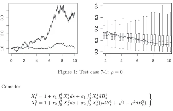
Figure 1: Test case 7-1: ρ = 0
Consider Xt1 = 1 + r1 Rt 0Xs1ds + σ1 Rt 0Xs1dBs1 X2 t = 1 + r2 Rt 0Xs2ds + σ2 Rt 0Xs2(ρdBs1+ p 1 − ρ2dB2 s) ) with σ1 = 0.1, σ2 = 0.2, r1 = 0.05 and r2 = 0.15. To simulate paths of (X1
t, Xt2) we have used the Euler scheme with stepsize 10−4. The
final time is T = 10. The observations are at times k · 10−2, 1 ≤ k ≤ 1000. In view of (45)
we consider the estimators
ξnt(1) = tL n t(2) Lnt(1)2, ξt(1) = t Lt(2) Lt(1)2 .
Figs. 1-4 are organized as follows: the left picture displays a particular sample path of the pair (Xt1, Xt2), and in the right picture we have plotted the paths of ξnt(1) (solid line) and ξt(1)) (dashed line) corresponding to the path of the left display. Moreover at each integer time t = 2, 3, · · · , 10 the right picture also displays two boxes and whiskers: the box and whiskers on the right plots the empirical quartiles and extends upward and downward to the extremal values of 500 independent samples of the random variables
ξnt(1); the box and whiskers on the left provides a similar information on ξt(1). Moreover the left-hand paths in all Figs 1-4 correspond to the same simulated path of the Brownian motion (B1, B2).
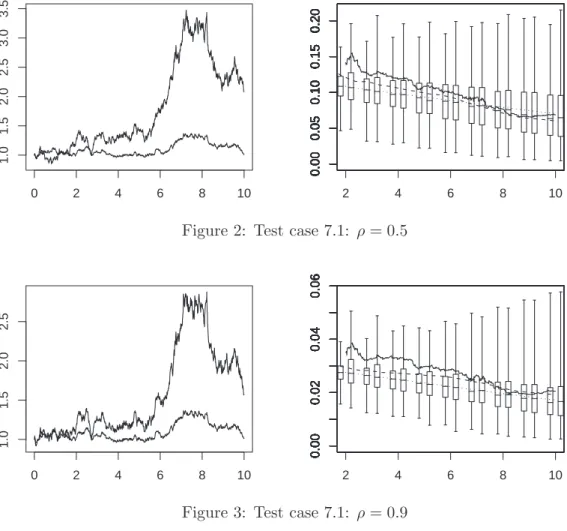
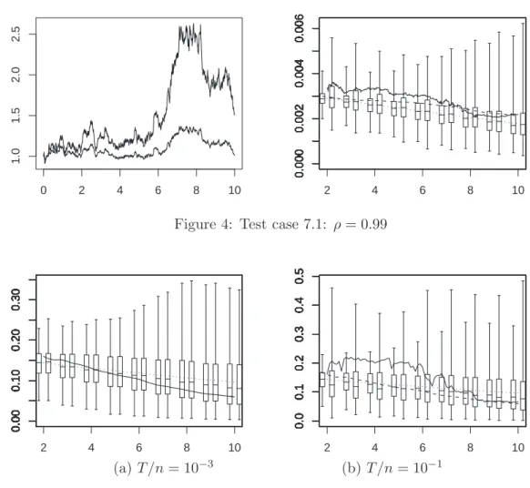
On this example we see that the paths of (X1, X2) for different values of ρ (and corresponding to the same Brownian motion (B1, B2)) are difficult to distinguish, whereas the values taken by ξnt(1) clearly allows one to distinguish the strongly correlated and weakly correlated cases.
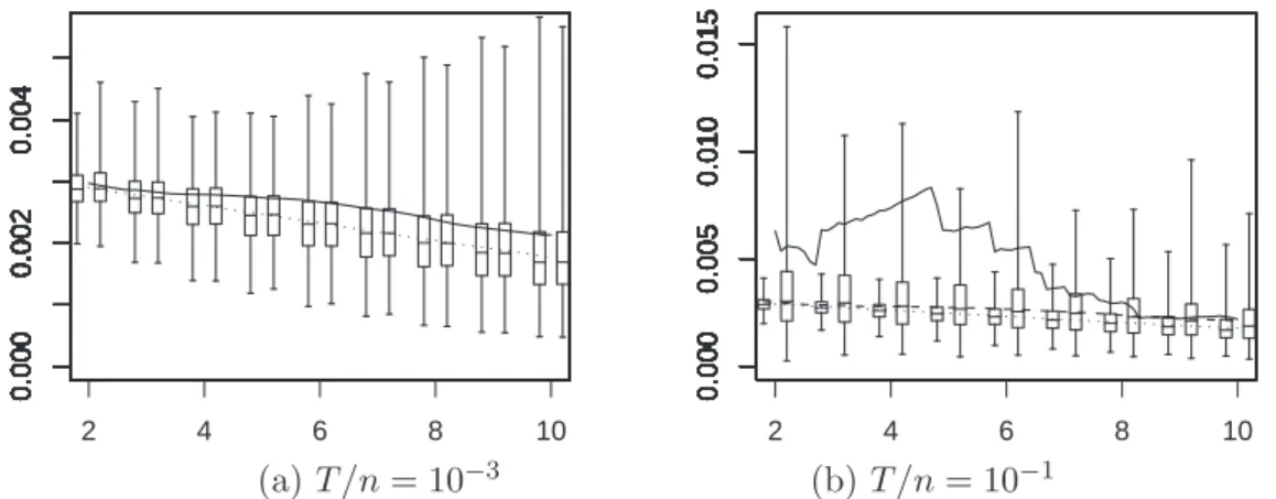
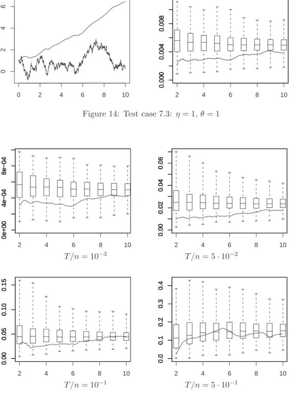
Figs. 5 and 6 display the same box and whiskers pictures than previously, but with
ρ = 0.00 and ρ = 0.99 and for two sampling frequencies T /n: for each integer time t the
left box and whiskers are the same on the left and right displays (they both are for ξt(1), beware the change of scale between the two displays), but unsurprisingly the spread of
ξnt(1) is bigger at low frequency (right display). However even at the lowest frequency (with only 100 observations) it allow to correctly estimate the real Brownian dimension.
0 2 4 6 8 10 1.0 1.5 2.0 2.5 3.0 3.5 2 4 6 8 10 0.00 0.05 0.10 0.15 0.20 0.00 0.05 0.10 0.15 0.20 0.00 0.05 0.10 0.15 0.20 0.00 0.05 0.10 0.15 0.20 0.00 0.05 0.10 0.15 0.20 0.00 0.05 0.10 0.15 0.20 0.00 0.05 0.10 0.15 0.20 0.00 0.05 0.10 0.15 0.20 0.00 0.05 0.10 0.15 0.20 0.00 0.05 0.10 0.15 0.20 0.00 0.05 0.10 0.15 0.20 0.00 0.05 0.10 0.15 0.20 0.00 0.05 0.10 0.15 0.20 0.00 0.05 0.10 0.15 0.20 0.00 0.05 0.10 0.15 0.20 0.00 0.05 0.10 0.15 0.20 0.00 0.05 0.10 0.15 0.20 0.00 0.05 0.10 0.15 0.20 0.00 0.05 0.10 0.15 0.20 0.00 0.05 0.10 0.15 0.20 0.00 0.05 0.10 0.15 0.20
Figure 2: Test case 7.1: ρ = 0.5
0 2 4 6 8 10 1.0 1.5 2.0 2.5 2 4 6 8 10 0.00 0.02 0.04 0.06 0.00 0.02 0.04 0.06 0.00 0.02 0.04 0.06 0.00 0.02 0.04 0.06 0.00 0.02 0.04 0.06 0.00 0.02 0.04 0.06 0.00 0.02 0.04 0.06 0.00 0.02 0.04 0.06 0.00 0.02 0.04 0.06 0.00 0.02 0.04 0.06 0.00 0.02 0.04 0.06 0.00 0.02 0.04 0.06 0.00 0.02 0.04 0.06 0.00 0.02 0.04 0.06 0.00 0.02 0.04 0.06 0.00 0.02 0.04 0.06 0.00 0.02 0.04 0.06 0.00 0.02 0.04 0.06 0.00 0.02 0.04 0.06 0.00 0.02 0.04 0.06 0.00 0.02 0.04 0.06
Figure 3: Test case 7.1: ρ = 0.9
7.2 A simplified model for energy indices
We now present a toy model for oil prices. In his Ph.D. thesis within a collaboration between INRIA and Gaz de France, O. Bardou [3] has studied modelling and simulation questions related to energy contract pricing problems. One question was to identify the co-efficients of a stochastic differential system which could satisfyingly describe the dynamics of about ten energy indices.
Here, for the sake of simplicity, we consider a three-dimensional system whose coeffi-cients resemble those identified by O. Bardou: for 1 ≤ i ≤ 3 we set
dXti= [αi(Xti− Ki)++ βi]dBit+ νi(µi− Xti)dt,
with X1
0 = 0.29, X02 = 0.89, X03 = 0.62.
Fixed this way, the diffusion term does not satisfy Hypothesis (H2). We thus slightly modify the equation and consider
dXti = [αiφ(Xti− Ki) + βi]dBti+ νi(µi− Xti)dt,
0 2 4 6 8 10 1.0 1.5 2.0 2.5 2 4 6 8 10 0.000 0.002 0.004 0.006 0.000 0.002 0.004 0.006 0.000 0.002 0.004 0.006 0.000 0.002 0.004 0.006 0.000 0.002 0.004 0.006 0.000 0.002 0.004 0.006 0.000 0.002 0.004 0.006 0.000 0.002 0.004 0.006 0.000 0.002 0.004 0.006 0.000 0.002 0.004 0.006 0.000 0.002 0.004 0.006 0.000 0.002 0.004 0.006 0.000 0.002 0.004 0.006 0.000 0.002 0.004 0.006 0.000 0.002 0.004 0.006 0.000 0.002 0.004 0.006 0.000 0.002 0.004 0.006 0.000 0.002 0.004 0.006 0.000 0.002 0.004 0.006 0.000 0.002 0.004 0.006 0.000 0.002 0.004 0.006
Figure 4: Test case 7.1: ρ = 0.99
2 4 6 8 10 0.00 0.10 0.20 0.30 0.00 0.10 0.20 0.30 0.00 0.10 0.20 0.30 0.00 0.10 0.20 0.30 0.00 0.10 0.20 0.30 0.00 0.10 0.20 0.30 0.00 0.10 0.20 0.30 0.00 0.10 0.20 0.30 0.00 0.10 0.20 0.30 0.00 0.10 0.20 0.30 0.00 0.10 0.20 0.30 0.00 0.10 0.20 0.30 0.00 0.10 0.20 0.30 0.00 0.10 0.20 0.30 0.00 0.10 0.20 0.30 0.00 0.10 0.20 0.30 0.00 0.10 0.20 0.30 0.00 0.10 0.20 0.30 0.00 0.10 0.20 0.30 0.00 0.10 0.20 0.30 0.00 0.10 0.20 0.30 2 4 6 8 10 0.0 0.1 0.2 0.3 0.4 0.5 0.0 0.1 0.2 0.3 0.4 0.5 0.0 0.1 0.2 0.3 0.4 0.5 0.0 0.1 0.2 0.3 0.4 0.5 0.0 0.1 0.2 0.3 0.4 0.5 0.0 0.1 0.2 0.3 0.4 0.5 0.0 0.1 0.2 0.3 0.4 0.5 0.0 0.1 0.2 0.3 0.4 0.5 0.0 0.1 0.2 0.3 0.4 0.5 0.0 0.1 0.2 0.3 0.4 0.5 0.0 0.1 0.2 0.3 0.4 0.5 0.0 0.1 0.2 0.3 0.4 0.5 0.0 0.1 0.2 0.3 0.4 0.5 0.0 0.1 0.2 0.3 0.4 0.5 0.0 0.1 0.2 0.3 0.4 0.5 0.0 0.1 0.2 0.3 0.4 0.5 0.0 0.1 0.2 0.3 0.4 0.5 0.0 0.1 0.2 0.3 0.4 0.5 0.0 0.1 0.2 0.3 0.4 0.5 0.0 0.1 0.2 0.3 0.4 0.5 0.0 0.1 0.2 0.3 0.4 0.5 (a) T /n = 10−3 (b) T /n = 10−1
Figure 5: Test case 7.1: ξnt(1) in terms of T /n (ρ = 0.00)
In this very simplified model the components of X are independent; in the real situation where one observes energy indices, one should take correlated Brownian motions Bi, as in
Subsection 7.1.
We set νi = µi = αi = 1. The drift term then stabilizes the process around the value
1. If βi= 0, the process (Xti) diffuses only when Xti is above the threshold Ki.
As above, we have approximated a path of the system by simulating the Euler scheme with stepsize 10−4 between times 0 and 10. The observations are at times k · 10−2, 1 ≤
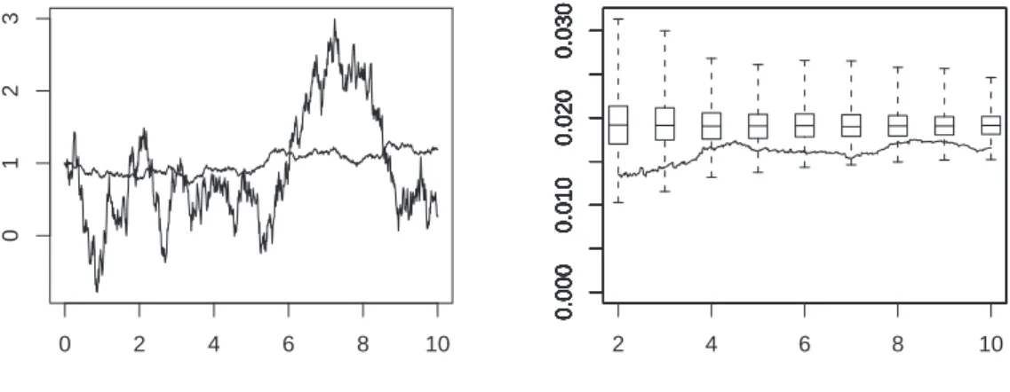
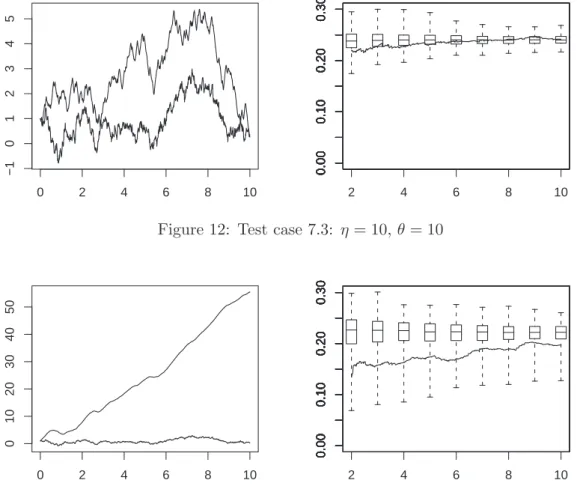
k ≤ 1000. In view of (45) we consider the estimators ξnt(1) = tL n t(2) Lnt(1)2, ξ n t(2) = √ t L n t(3) Lnt(2)3/2, and ξt(1) = tLt(2) Lt(1)2 , ξt(2) =√t Lt(3) Lt(2)3/2 .
2 4 6 8 10 0.000 0.002 0.004 0.000 0.002 0.004 0.000 0.002 0.004 0.000 0.002 0.004 0.000 0.002 0.004 0.000 0.002 0.004 0.000 0.002 0.004 0.000 0.002 0.004 0.000 0.002 0.004 0.000 0.002 0.004 0.000 0.002 0.004 0.000 0.002 0.004 0.000 0.002 0.004 0.000 0.002 0.004 0.000 0.002 0.004 0.000 0.002 0.004 0.000 0.002 0.004 0.000 0.002 0.004 0.000 0.002 0.004 0.000 0.002 0.004 0.000 0.002 0.004 2 4 6 8 10 0.000 0.005 0.010 0.015 0.000 0.005 0.010 0.015 0.000 0.005 0.010 0.015 0.000 0.005 0.010 0.015 0.000 0.005 0.010 0.015 0.000 0.005 0.010 0.015 0.000 0.005 0.010 0.015 0.000 0.005 0.010 0.015 0.000 0.005 0.010 0.015 0.000 0.005 0.010 0.015 0.000 0.005 0.010 0.015 0.000 0.005 0.010 0.015 0.000 0.005 0.010 0.015 0.000 0.005 0.010 0.015 0.000 0.005 0.010 0.015 0.000 0.005 0.010 0.015 0.000 0.005 0.010 0.015 0.000 0.005 0.010 0.015 0.000 0.005 0.010 0.015 0.000 0.005 0.010 0.015 0.000 0.005 0.010 0.015 (a) T /n = 10−3 (b) T /n = 10−1 Figure 6: Test case 7.1: ξnt(1) in terms of T /n (ρ = 0.99)
0 2 4 6 8 10 −1 0 1 2 3 2 4 6 8 10 0.0 0.1 0.2 0.3 0.4 0.0 0.1 0.2 0.3 0.4 0.0 0.1 0.2 0.3 0.4 0.0 0.1 0.2 0.3 0.4 0.0 0.1 0.2 0.3 0.4 0.0 0.1 0.2 0.3 0.4 0.0 0.1 0.2 0.3 0.4 0.0 0.1 0.2 0.3 0.4 0.0 0.1 0.2 0.3 0.4 0.0 0.1 0.2 0.3 0.4 0.0 0.1 0.2 0.3 0.4 0.0 0.1 0.2 0.3 0.4 0.0 0.1 0.2 0.3 0.4 0.0 0.1 0.2 0.3 0.4 0.0 0.1 0.2 0.3 0.4 0.0 0.1 0.2 0.3 0.4 0.0 0.1 0.2 0.3 0.4 0.0 0.1 0.2 0.3 0.4 0.0 0.1 0.2 0.3 0.4 0.0 0.1 0.2 0.3 0.4 0.0 0.1 0.2 0.3 0.4 0.0005 0.2268
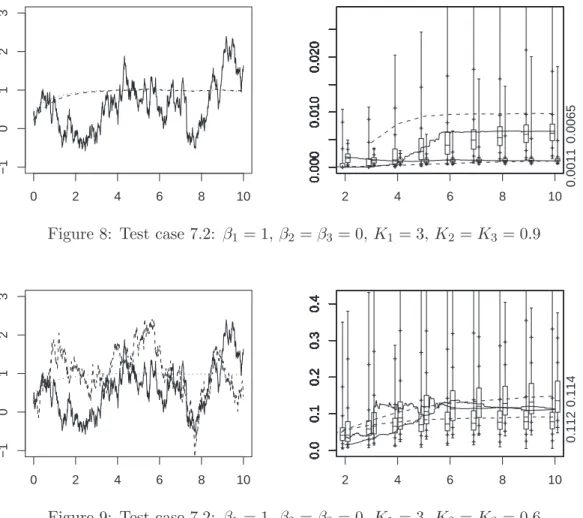
Figure 7: Test case 7.2: β1= β2 = 1, β3 = 0, K1 = K2 = 3, K3 = 0.9
the corresponding paths of ξnt(j) (solid line) and ξt(j) (dashed line), for j = 1 and j = 2: respectively the top and the bottom curves; values on the right hand-side vertical axes denote ξnT(1) and ξnT(2). Moreover on the right we have box and whiskers for the empirical quartiles of ξnt(1) (top) and ξnt(2) (bottom), computed from 500 independent paths and for all integer times t = 2, 3, · · · , 10. The whiskers extend to the extremal values of the samples, the other ticks denoting the 1 %, 10 %, 90 % and 99 % quantiles.
In Fig.7, the two first components diffuse from time 0 to time 10 since K1 and K2 are large. The third component diffuses a little only since it is attracted to 1 and φ(1 − K3) = φ(0.1) is small. Given the threshold ρn= 0.01, the explicative Brownian dimension Ren,t
is 2 since ξnt(1) takes values around 0.2 whereas ξnt(2) takes values around 2 10−3. In Fig. 8, the two last components have a small diffusion term. As both ξnt(1) and
ξnt(2) take values less than 0.02, according to the same threshold ρn= 0.01 as above, the
explicative Brownian dimension Ren,t is 1.
In Fig. 9, we have K1 large, and φ(1 − K2) = φ(1 − K3) = φ(0.4) = 0.3. Therefore none of the diffusion terms can be neglected, but the first component ‘oscillates’ more