HAL Id: hal-02989427
https://hal.archives-ouvertes.fr/hal-02989427
Submitted on 5 Nov 2020HAL is a multi-disciplinary open access
archive for the deposit and dissemination of sci-entific research documents, whether they are pub-lished or not. The documents may come from teaching and research institutions in France or abroad, or from public or private research centers.
L’archive ouverte pluridisciplinaire HAL, est destinée au dépôt et à la diffusion de documents scientifiques de niveau recherche, publiés ou non, émanant des établissements d’enseignement et de recherche français ou étrangers, des laboratoires publics ou privés.
Tackling Solvent Effects by Coupling Electronic and
Molecular Density Functional Theory
Guillaume Jeanmairet, Maximilien Levesque, Daniel Borgis
To cite this version:
Guillaume Jeanmairet, Maximilien Levesque, Daniel Borgis. Tackling Solvent Effects by Coupling Electronic and Molecular Density Functional Theory. Journal of Chemical Theory and Computation, American Chemical Society, 2020, �10.1021/acs.jctc.0c00729�. �hal-02989427�
Tackling solvent effects by coupling electronic
and molecular Density Functional Theory
Guillaume Jeanmairet,
⇤,†Maximilien Levesque,
¶and Daniel Borgis
¶†Sorbonne Université, CNRS, Physico-Chimie des Électrolytes et Nanosystèmes Interfaciaux, PHENIX, F-75005 Paris, France.
‡Réseau sur le Stockage Électrochimique de l’Énergie (RS2E), FR CNRS 3459, 80039 Amiens Cedex, France
¶PASTEUR, Département de chimie, École normale supérieure, PSL University, Sorbonne Université, CNRS, 75005 Paris, France
§Maison de la Simulation, CEA, CNRS, Université Sud, UVSQ, Université Paris-Saclay, 91191 Gif-sur-Yvette, France
E-mail: [email protected]
Abstract
Solvation effects can have a tremendous influence on chemical reactions. However, precise quantum chemistry calculations are most often done either in vacuum neglect-ing the role of the solvent or usneglect-ing continuum solvent model ignorneglect-ing its molecular nature. We propose a new method coupling a quantum description of the solute using electronic density functional theory with a classical grand-canonical treatment of the solvent using molecular density functional theory. Unlike previous work, both densit-ies are minimised self-consistently, accounting for mutual polarisation of the molecular solvent and the solute. The electrostatic interaction is accounted using the full electron density of the solute rather than fitted point charges. The introduced methodology rep-resents a good compromise between the two main strategies to tackle solvation effects
in quantum calculation. It is computationally more effective than a direct quantum-mechanics/molecular mechanics coupling, requiring the exploration of many solvent configurations. Compared to continuum methods it retains the full molecular-level de-scription of the solvent. We validate this new framework onto two usual benchmark sys-tems: a water solvated in water and the symmetrical nucleophilic substitution between chloromethane and chloride in water. The prediction for the free energy profiles are not yet fully quantitative compared to experimental data but the most important features are qualitatively recovered. The method provides a detailed molecular picture of the evolution of the solvent structure along the reaction pathway.
1 Introduction
The solvent is often described as the media in which a chemical reaction between dissolved species, called solutes, takes place. However, it is well known that besides its role of bringing the reactants in contact, the solvent has a tremendous influence on the chemical reaction as it impacts the kinetics and the thermodynamics of the reaction. Organic chemists have taken advantage of these solvent effects since decades. For instance, in the 30’s, Hughes and Ingold already discussed a theory of solvation effects for nucleophilic substitution (SN)1. In this paper, they reviewed the already substantial experimental work on the influence of the choice of solvent on the SN reaction and they proposed a theoretical model accounting for solvent effects. Hughes and Ingold model is based on a simple hypothesis: only electrostatic interactions are considered. By examining the stabilising and/or destabilising role of the solvent on the reactants, products and transition states of the reaction they were able to rationalise effects of solvent polarity on reaction rates. However, solvent molecules may also be directly involved in the reaction mechanism. For instance, Liu et al have shown that adding a single methanol molecule largely promotes the SNreaction with respect to elimina-tion reacelimina-tion2. Direct involvement of solvent molecules cannot be captured by macroscopic consideration as the ones used in Hughes and Ingold model. A good alternative is to
re-sort to molecular simulation. Since chemical reaction involves formation and/or breaking of chemical bonds it makes the use of classical force fields difficult: even if reactive force fields exist, their parametrisation are often costly and laborious3,4. Thus, to study chemical reactions the first approach is often to use a Quantum Mechanics (QM) based method such as electronic density functional theory (eDFT), Hartree Fock or more advanced techniques such as Moller-Plesset or Coupled Cluster. Due to computational cost, such calculations are often run in vacuum and at 0 K which neglect solvent effects.
To incorporate solvent effects, the most natural choice is to explicitly include solvent molecules into the simulation. This is extremely costly since it increases considerably the number of electrons with respect to in vacuo calculations. The finite temperature is even more problematic since the meaningful quantity is no longer the ground state energy but the free energy. This means that the calculation should take place in a statistical ensemble and that a long enough trajectory should be produced to compute ensemble average with good statistics5. This is the typical setup of ab-initio Molecular Dynamics (AIMD) calculations6. The problem of free energy calculation is particularly difficult since it cannot be written as a (grand) canonical average over the phase space5. For those two reasons AIMD simulations are limited to efficient QM techniques. There are almost always based on eDFT and only small systems can be investigated.
To circumvent the computational cost of AIMD a natural choice is to split the studied system into 2 parts. A first one, which is considered as essential for the description of the chemistry is treated at the QM level. A second one, which often includes most of the solvent molecules, for which interactions are described by molecular mechanics (MM) using classical force fields. This is the well known QM/MM approach which has been used successfully to tackle a wide variety of systems7. The MM part is most often dealt with Molecular Dynamics (MD) or Monte Carlo (MC). While QM/MM makes it possible to considerably reduce the numerical cost of evaluating forces as compared to AIMD, the problem of computing free energy remains. A further simplification is to average out the solvent degrees of freedom to
reduce tremendously the dimensionality of the problem and the computational cost. This is the strategy adopted in continuum solvent models (CSM) approaches such as the polarisable continuum model (PCM)8–10 where the solvent is described by a dielectric continuum. CSM have been applied with success but they suffer from several drawbacks. First, they con-tain ah-hoc parameters that are not physically based but are rather optimised on reference calculations. Second, they completely lose the description of the solvent at the molecular level.
Another way to tackle solvation problem is to conserve the QM/MM partition of the system but to use liquid state theories to deal with the MM part. Liquid state theories have proven efficient to describe simple liquids such as hard-sphere or Lennard-Jones fluids11. Several approaches among which integral equation theory, its interaction site approximation (RISM)12 or classical density functional theory (cDFT)13 have been applied in that context. The common objective of all these techniques is to find the equilibrium number solvent density n(r), or equivalently its total correlation function h(r). For simple liquids these fields solely depends on the position of the solvent r. A key quantity entering all these theories is the direct correlation function between solvent molecules c(r).
More recent developments have made possible to tackle realistic molecular fluids such as water or acetonitrile, either based on the integral equation theory14 or the molecular density functional theory (MDFT)15–22. In a molecular solute-solvent system the density field ⇢(r, ⌦) no longer depends solely on the position r but also on the orientation ⌦ of the solvent. Consequently the direct correlation function c(r, ⌦1, ⌦2) becomes extremely complicated as it now depends on a position vector and two orientations.
The RISM approach and its 3D-RISM23 generalisation circumvent this problem by av-eraging out the solvent orientation. The complicated molecular correlation function c is replaced by simpler 1D site-site correlation functions. The gain in efficiency is obvious but it is at the price of working with site-site OZ equation and site-site correlation functions which are no longer based on a proper statistical physics derivation. Another approach based on
molecular density functional theory (MDFT) has ben proposed recently to solve the MOZ equation, with the hypernetted chain (HNC) closure, without making such approximations. The use of projections onto rotational invariants allows to handle the numerically costly angular convolution products24 making the method practical.
Liquid state theories represent a good compromise between CSM and MD based ap-proaches since they conserve the description of solvent as made of molecular entities while not requiring the tedious statistical sampling of solvent degrees of freedom. It is thus natural to propose a formalism where solutes are described using QM and solvent using liquid state theories. Since the original paper25, numerous studies using RISM26 or 3D-RISM27–30 have been carried out to study solvation effects on a solute described by QM. This method is implemented in widely distributed quantum codes such as ADF31,32. Because the develop-ments of classical DFT techniques to study molecular liquids are more recent, less attempts have been made to describe solvation of QM solutes with this method. The Arias group have developed the joint DFT framework33,34 and released the code JDFTx35 where the method is implemented. The functionals implemented in JDFTx are describing model fluids, they are parametrised to reproduce some features of the real molecular liquid such as its non-local dielectric response on external electric field —an improvement over PCM. However the performance of this simplified DFT approach to reproduce molecular properties is not completely satisfying36,37.
Zhao et al recently proposed the so-called Reaction Density Functional Theory (RxDFT)38–40 which is based on MDFT. In this approach the solute energy is computed using eDFT. Then the solute is described classically by a set of Lennard-Jones sites and point charges in a sub-sequent MDFT calculation to estimate the solvation free energy. The classical charges are fitted to reproduce the molecular electrostatic potential (ESP) computed in the QM calcula-tion. This is a first limitation since there is no unique way to determine the ESP charges as illustrated by the variety of existing fitting methods41–43. Another limitation is the absence of polarisation of the QM solute under the influence of non homogeneous solvent density
in RxDFT. The ESP charges are fitted using electronic densities computed in vacuum or using a CSM. This method thus actually consists in a MDFT calculation with a force field where the charges have been reparametrised on a prior eDFT calculation rather than in a self-consistent QM/MDFT procedure.
The purpose of this paper is to address these limitations and to propose a QM/MDFT procedure where the quantum part and the MDFT part are optimised self-consistently. Moreover, in contrast to the common practise in QM/MM approaches, the solute electronic density is directly used in the MDFT calculation which prevent to use ill-defined atomic point charges. The rest of the paper is organised as follow, first we present the theoretical aspects of the coupling between QM and MDFT before testing the proposed methodology on two commonly-used benchmarks. We first focus on the solvation of an eDFT water molecule in MDFT water before addressing an aqueous chemical reaction namely a symmetric nucleophilic substitution between chloromethane and chloride.
2 Theory
The solvation free energy (SFE) F can be defined as the difference between the free energy of the solute-solvent system and the sum of the free energies of the solute in vacuum and of the pure solvent as depicted in figure 1.a. It is a key quantity to understand chemistry in solution. For instance, the SFE difference between the products and the reactants, figure 1.b, is directly linked to the equilibrium constant of the reaction. Similarly, the difference between the SFE of the same solute in two different solvents allows to compute partition constant. The aim of this paper is to propose a joint self-consistent eDFT/MDFT approach to evaluate the SFE.
We start by our standard formulation of molecular density functional theory. In MDFT, the solvent molecules are assumed to be rigid entities interacting through a classical force field. Since molecules are rigid, the knowledge of the position of their centre of mass (COM) r
+
+
+
-Fa Fb
a)
b)
Figure 1: Thermodynamic scheme for the computation of solvation free energy (left) and reaction free energy (right). The electronic density of the solute is schematised by a solid black line. Dashed line represents the electronic density in the previous state.
and their orientation ⌦ are sufficient to fully describe molecule coordinates. In this paper we only consider SPC/E water as a solvent but we proposed functionals for other molecular fluids such as acetonitrile in the past44. The DFT ansatz states that for any external perturbation it is possible to write a unique functional F of the solvent density ⇢45. At its minimum, which is reached for the equilibrium density ⇢eq, the functional F equals the SFE F . MDFT is thus particularly appropriate to compute SFE since it requires a functional minimisation while brute force MD would require a costly sampling. The functional F is usually written as
F [⇢] = Fid[⇢] + Fext[⇢] + Fexc[⇢]. (1) The solvent density ⇢(r, ⌦) is a 6D field that depends on the space coordinate and the orientation ⌦.
In equation 1 the ideal term Fid corresponds to the entropic term of the non-interacting fluid11. The third term Fexc is due to solvent-solvent interaction18. In this work we use the expression proposed by Ding et al for SPC/E24, which corresponds to the so-called hypernetted-chain closure for the excess functional Fexc. The remaining term Fext is due to the external perturbation acting on the liquid, here the solute. This last term represents the solute-solvent interaction and can formally be written as
Fext[⇢] = ZZ
where Vext is the external energy density.
In our previous work17–22,46the solute was described by a classical force field, usually a set of Lennard-Jones sites and point charges. Here we describe the solute quantum mechanically using eDFT. Using the DFT ansatz47, it exists a functional Fe of the electronic density ⇢e which is equal to the ground state energy at its minimum, it is usually approximated as48
Fe[⇢e] = Ts[⇢e] + Z
Vne[r]⇢e(r)dr + EH[⇢e] + EXC[⇢e] (3) where Ts is the non-interacting kinetic-energy functional, Vne is the external potential due to the nuclei acting on the electrons, EH is the Hartree functional and EXC the exchange-correlation functional. The electrostatic interaction between the quantum solute and the classical solvent can easily be expressed in a mean field way
EES[⇢, ⇢e] = ZZ
V(r) U(r0) 4⇡✏0|r r0|
drdr0 (4)
where Vis the charge density of the solvent and Uis the charge density of the solute. Each of these charge densities is related to the corresponding particle density. The solute charge density is
U(r) = X
i
Zi (r ri) ⇢e(r) (5) where Zi is the atomic number of nucleus i located in ri. The solvent charge density can be expressed as
V(r) = ZZ
⇢(r, ⌦) (r r0, ⌦)dr0d⌦. (6) where (r, ⌦) is the charge density of a water molecule taken at the origin with orientation ⌦.
The electrostatic contribution to the external term of equation 2 can be computed inject-ing equations 5-6 in equation 4. However, short-range repulsion and dispersion interactions are not taken into account. To do so, similarly to QM/MM calculations, we resort to
Lennard-Jones sites located on nuclei of the solute. Since there is no prescription on how to choose the Lennard-Jones parameters the common practice is to resort to generic force fields such as OPLS49 or CHARMM50. However, the solvation free energy and the solvation structure depend on the LJ parameters50,51. That is why, as any QM/MM calculation, the present approach cannot be considered as being truly ab initio. A more elegant and ab initio way would be to use some electron-solvent pseudo-potential to account for the repulsion-dispersion interactions52. This strategy has been widely applied to study solvated electrons in liquids or clusters53–56. Eventually, the external term of the functional can be written as
Fext[⇢, ⇢e] = EES[⇢, ⇢e] + ZZ ⇢ (r, ⌦) VLJ(r, ⌦)drd⌦. (7) with VLJ(r, ⌦) = X i2solute X j2solvent 4✏ij "✓ ij |r + rj⌦ ri| ◆12 ✓ ij |r + rj⌦ ri| ◆6#
where ✏ij and ij are the mixed Lennard-Jones parameters using the Lorentz-Berthelot rules, ri is the position of the ith site of the solute and rj⌦ denotes the position with respect to the COM of site j of a solvent molecule located in r with orientation ⌦.
As opposed to our previous work where the solute was described classically, the free energy of the solute is modified when transferred from the gas phase to the solute. We approximate this free energy difference FQM by the energy difference at T = 0 K which is much easier to compute. This neglects the nuclear and electronic fluctuations.
FQM[⇢e]⇡ EQM[⇢e] = Fe[⇢e] Fe[⇢vace ] (8) where ⇢vac
8 the solvation free energy can be computed by minimising the functional
F [⇢e, ⇢] = EQM[⇢e] + Fid[⇢] + Fext[⇢e, ⇢] + Fexc[⇢] (9) with respect to the electronic density ⇢e(r) and the solvent density ⇢(r, ⌦).
Instead of carrying the joint minimisation we adopt a simpler strategy. First, the elec-tronic functional is minimised in vacuum. The equilibrium elecelec-tronic density is then used in the MDFT calculation to compute the electrostatic contribution to external term using equa-tion 4. After minimisaequa-tion of the MDFT funcequa-tional, the equilibrium solvent charge density is used to compute the electrostatic external potential acting on the electronic density using equation 4. The electronic functional is minimised and a new electronic density is obtained. This process is repeated until both the electronic energy of equation 8 and the solvation free energy of equation 1 are converged to a given threshold. Using this procedure, the electrostatic energy of equation 4 is computed twice, once in the electronic DFT calculation and once in the MDFT one. These two values can be compared as a sanity check to verify convergence.
We insist on the fact that the full electronic density of the quantum solute is used in the computation of electrostatic interaction between the QM and the MM part in equation 4. It differs from the strategy usually adopted in QM/MM calculations that consists in computing partial point charges from the electronic density7. Since there is no unique way to determine these charges41,42,57 and since it is difficult to evaluate their quality a posteriori it is advantageous to circumvent this parametrisation and work directly with the electronic density.
The self-consistent optimisation of electronic density ⇢e(r)and the solvent density ⇢(r, ⌦) when minimising equation 9 allows to account for the mutual polarisation of the solute and the solvent environment. This is a clear improvement with respect to methods that consist in a single QM calculation in vacuum followed by a single liquid state theory calculation such
as RxDFT38–40. Indeed, such methods neglect the polarisation of the solute by the solvent density which is properly accounted with the present approach.
A last strength of the present approach is that it retains a proper description of the solvent at the molecular level. The equilibrium solvent density contains a detailed 3D picture of the solvent location and orientations around the solute which is not accessible to continuum models or simpler liquid state theories.
3 Applications
3.1 Water in water.
As a first test of the QM/MDFT framework introduced in 2, we focus on the “water in water” system. A single water molecule, referred as the solute, is immersed in water solvent described by MDFT. The solute is treated at the eDFT level with the PBE functional. Calculations are run using the GPAW package58–60. Wave functions are expanded on a real space grid. The volume of the simulation cell is 5 ⇥ 5 ⇥ 5 Å3 and details about the grid resolution are given below. The geometry of the solute is the one of the SPC/E molecule.
Solvent calculations are done using our homemade MDFT code, the water model is SPC/E. We used a cubic cell of 25 ⇥ 25 ⇥ 25 Å3. The orientational space SO(3) is discretised with 196 orientations, the space grid resolution is specified further. Our homemade fortran written MDFT program was interfaced with Python using f90wrap which makes the coupling with GPAW easy.
Dispersion-repulsion forces are modelled using Lennard-Jones sites located on the solute atoms in the MDFT calculation. The Lennard-Jones parameters of the oxygen of the solute are the same as in SPC/E. The Lennard-Jones parameters on hydrogens are = 1.0 Å and ✏ = 0.0234 kJ.mol 1. This almost non attractive Lennard-Jone site prevent numer-ical divergence due to “unshielded” charges, this trick has already been used in RISM-SCF studies25,61.
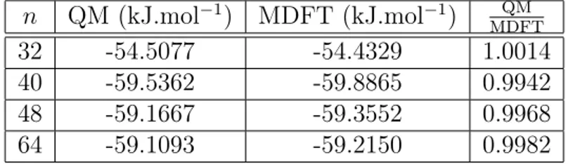
We first check the validity of the implementation by comparing the external electrostatic energies obtained in the QM and in the MDFT calculations according to equation 4. For this test there are n3 points in the QM grid and 8 n3 in the MDFT one where n = 32, 40, 48, 64. The convergence criterion on the relative variation is 10 4 for both the QM energy and the MDFT free energy. Results are reported in table 1. In all cases the electrostatic energies agree within 1%. For n = 32 the resolution of the grids are clearly not sufficient since the results differ by 5 kJ.mol 1 from the one obtained with finer grids. If n = 32 is omitted, the finer the grid the better is the agreement between the two ways to evaluate the electrostatic energy.
Table 1: Final external electrostatic energy of water in water computed according to equation 4. The second column is the result obtained with the QM code, the result obtained with MDFT is displayed in the third column. The fourth column shows the ratio of the second and third column. There are n3 nodes on the QM grid and 8n3 on the MDFT grid.
n QM (kJ.mol 1) MDFT (kJ.mol 1) QM MDFT 32 -54.5077 -54.4329 1.0014 40 -59.5362 -59.8865 0.9942 48 -59.1667 -59.3552 0.9968 64 -59.1093 -59.2150 0.9982
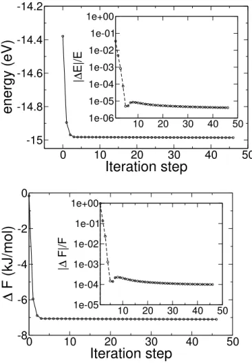
After this numerical test we run calculation on the same system with 483 grid nodes on the QM grid and 1203nodes on the MDFT space grid. We use a convergence criterion of 10 4 on the relative variation of QM energy and MDFT free energy. The electronic energies and solvation free energies as a function of the iteration step are displayed in figure 2. It requires 42 iterations to reach a criterion of 10 4 and only 5 iterations are necessary to converge within 10 3. As expected, solvation stabilises the solute: the QM energy at convergence is 0.58 eV lower than in the initial state i.e. in vacuum. In a similar way, the solvation free energy computed by MDFT is reduced by 6.6 kJ.mol 1 when the electronic density is optimised.
Moreover, the polarisation of the solvent influences the electronic density of the solute. This effect can only be captured if the electronic density and the solvent density are optimised
self-consistently. 0 10 20 30 40 50
Iteration step
-15 -14.8 -14.6 -14.4 -14.2energy (eV)
10 20 30 40 50 1e-06 1e-05 1e-04 1e-03 1e-02 1e-01 1e+00 |∆ E|/E 0 10 20 30 40 50Iteration step
-8 -6 -4 -2 0∆
F (kJ/mol)
10 20 30 40 50 1e-05 1e-04 1e-03 1e-02 1e-01 1e+00 |∆ F|/FFigure 2: Energy of the quantum solute as computed by eDFT (top) and its solvation free energy as computed by MDFT (down) as a function of the iteration step. In insets are the relative differences of these quantities.
The solvation free energy of water computed using equation 9 is 3.4 kJ.mol 1. It is clearly overestimated when compared to the experimental value of 26.5 kJ.mol 1 but also to the value of 29.5 kJ.mol 1 which is the one of the SPC/E model computed using MD. Using the continuum solvent model implemented in GPAW62 gives a solvation free energy of 27.0 kJ.mol 1 in better agreement with the experimental value. The overestimation of solvation free energy is a known problem of the HNC functional as already illustrated for the TIP3P model63 and is mostly due to the quadratic form of the functional, which causes a tremendous overestimation of the pressure17,19. We have proposed several physically based
bridge functionals to correct this flaw and go beyond the HNC level. It is also possible to stay at the HNC level and simply use a one parameter a posteriori cavity correction of the SFE63. Using this simple correction, we obtain a solvation free energy of 20.2 kJ.mol 1, in better agreement with the experimental value but still overestimated.
Unfortunately, the imperfection of the functional is not the sole defect of our calculation. Predictions of the solvation free energy are also quite sensitive to the choice of Lennard-Jones parameters. To illustrate this point we computed the solvation free energy of water changing only the Lennard-Jones site on the oxygen of the solute. We have taken the values of and ✏ from some popular water models: SPC/E, OPC, TIP3P and TIP4P. We emphasise that the geometry of the solute is not changed. The SFE computed using these parameters are displayed in table 2 and they vary by up to 1.5 kJ.mol 1.
Table 2: Solvation Free energy of water obtained using different Lennard-Jones parameters for the solute described using eDFT. The geometry is always the one of SPC/E.
Å ✏ (kJ.mol 1) F (kJ.mol 1) TIP3P 3.15061 0.6364 -20.3 TIP4P 3.1589 0.7749 -19.5 OPC3 3.165 0.9945 -18.8 SPC/E 3.17427 0.65 -20.2
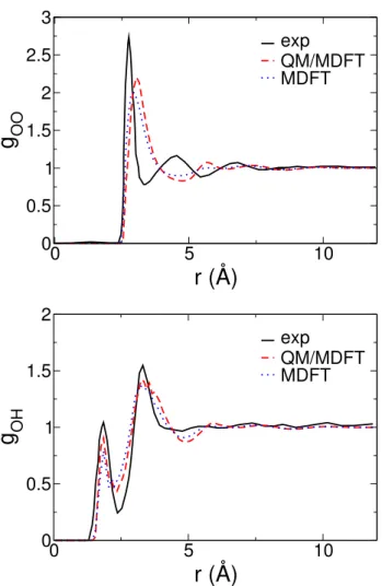
After examining the energetics, we now turn to the solvation structure. The radial distribution functions (rdf) between oxygen of the solvent and atomic sites of the solute are displayed in figure 3. First, we recall that the agreement between the experimental rdf and the one computed by MD for the SPC/E model is good64,65. The agreement is less satisfying for the rdf predicted by MDFT using the HNC functional as previously reported for SPC/E and TIP3P18,63. Indeed, the first peak of the OO rdf is overestimated and slightly shifted toward the long distances while the second and third peaks are underestimated and markedly shifted toward the long distances. The agreement is much better for the OH rdf since the two first peaks are found at the right places even if there are underestimated as is the depletion between the two peaks. Since the present approach uses the HNC functional
with no modifications, the same defects are found on the rdf computed using the QM/MDFT framework. Using a quantum solute tends to improves the intensity of the peaks: the two first peaks of the OH and OO rdf increase. However the peaks of the OH rdf are still underestimated and the depletion between the two first peaks of the OH rdf remains too small. Considering the position of the peaks, there is no improvement on the OH rdf and it even worsen the OO rdf where the first maximum is shifted further toward the large distances.
Overall the radial distribution functions computed using the QM/MDFT approach re-main similar to the one obtained using MDFT on a classical SPC/E solute. We can expect that bridge functionals improving the structural properties on classical systems to be trans-ferable to QM/MDFT calculations.
While rdf function is a practical way to examine solvation structure it only contains spherically averaged information. This is not the case of the 3D densities that can be com-puted with MDFT. We estimate the solvent charge CSMusing the CSM model implemented in GPAW62 and compare it to the 3D solvent charge density
V given by equation 6. We assume that the whole difference between the electrostatic potential in CSM, ES
CSM and the one in vacuum ES
vac is due to the electrostatic potential generated by solvent ESV ES
V = ESCSM ESvac. (10) This electrostatic potential ES
V is linked to the solvent charge CSM through a Poisson equation
ES
V = CSM✏
0 (11)
where ✏0 is the vacuum permitivitty.
Of course the charge density CSMactually does not solely contain the contribution due to the dielectric response of the solvent. The modification of the electronic density also impacts the electrostatic potential. Moreover, in equation 11 we simply used the vacuum permitivitty
0 5 10
r (Å)
0 0.5 1 1.5 2 2.5 3g
OO exp QM/MDFT MDFT 0 5 10r (Å)
0 0.5 1 1.5 2g
OH exp QM/MDFT MDFTFigure 3: Radial distributions functions between the O site of the solvent and the O (top) or H (down) site of the solute. Results of the HNC functional for the classical SPC/E solute are in dotted blue while the one obtained with a QM solute are in dashed red. For comparison we reported the experimental results by Soper in full black64.
while we should have used the spatially varying permittivity entering the continuum model. Thus, the charge density CSM is simply a qualitative tool to visualise solvation effects in the CSM calculation.
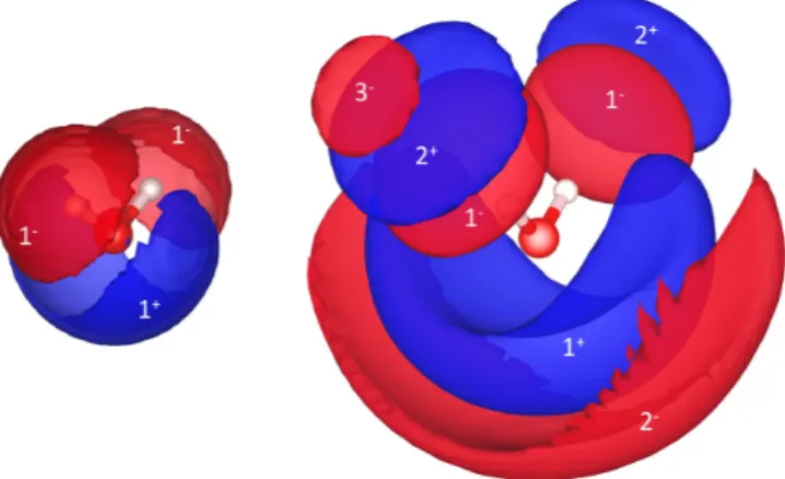
In figure 4 we compare the charge densities obtained with CSM and with MDFT. The solvent charge density V predicted by MDFT is more structured than CSM: there are additional lobes. To ease the discussion, we identify the lobes in figure 4 by their distances with respect to the centre of mass of the solute. The closest positive lobe is denoted 1+, the second negative 2 , etc.
The lobes 1+ and 1 are similar in the CSM calculation and in the MDFT calculation. However, the charge distribution obtained by CSM is located on the cavity surface while the lobes obtained with MDFT have 3D shapes.
1+ and 1 correspond to the first solvation shell and not surprisingly we observe that the solvent is polarised such as positive charges appear close to the oxygen atom while negative charges develop close to the hydrogen atoms. In the MDFT results, a second set of lobes exists. They have a shape similar to the one of the first lobes but with opposite charges and they are located in their vicinity, e.g. 2+ is close to 1 . We estimated the distance between 1+ and 2 and between 2+ and 1 by measuring distances between several pairs of points pertaining to each isosurface. We found that both pairs of isosurfaces are roughly distant by 1Å. This is of the order of the OH bond length in the SPC/E water model, thus each pairs of oppositely charge isosurface belong to the first solvation shell of water. We recover the tetrahedral order with preferential orientation of water around the water solute molecule.
While the dipole moment of the water molecule is well known to be 1.85 D in the gas phase66 its value in the liquid have been more controversial with simulation prediction ran-ging from 2.1 to 3.1 D67. In the beginning of the 2000’s several independent experimental studies have found a value of 2.9-3.0 D for the dipole moment in the liquid67,68. In table 3 we display the dipole moment of a water molecule in gas and liquid phase. We obtain a dipole of 1.9 D with the PBE functional, in good agreement with the experimental value in
Figure 4: Isosurfaces of solvent charge densities: positive surfaces are displayed in blue and negative ones in red. The left figure have been obtained with the CSM calculation using equation 11. The right one have been obtained with MDFT with equation 6.
vacuum. The value in solution is estimated to 2.3 D with the continuum solvation model. This is clearly underestimated with respect to the experimental value but this falls within the range of values predicted using simulations and QM/MM approaches69. Note that this value is interestingly close to 2.35 D which is the one of the SPC/E model65. With the MDFT approach we do obtain an enhancement of the dipole of the water molecule in solution. After a single MDFT calculation most of the polarisation is recovered with a dipole of 2.2 D. After converging the self-consistent cycle, the dipole increases to 2.3 D. Once again, this shows the importance of the self-consistent optimisation of electronic and solvent densities to account for their mutual polarisation.
Note that the same value of the dipole is obtained using any of the Lennard-Jones para-meters of table 2. It should be noted that several AIMD simulations of liquid water using the PBE functional have found a dipole value of 2.9-3.2 D70,71 which is in good agreement with experiments. The underestimation of the dipole moment in the liquid phase in the MDFT calculation may have several origins. First, it has been demonstrated using ab initio MD that the dipole moment of rigid water molecules tends to be smaller than when the geo-metry is allowed to relax70. Second, as opposed to AIMD there is no electronic polarisation of the solvent molecules since we use a non-polarisable model. A third reason might be the limitation of the HNC functional. As illustrated in figure 3, the first peak of the oxygen
rdf is broadened, reduced and shifted further from the solute with the HNC functional with respect to experiments while the hydrogen rdf more or less agree. Consequently, the charge distribution of the solvent predicted by the HNC functional is smoother. As a consequence, the electric field generated by the solvent is reduced and the water solute is less polarised than in experiment.
Table 3: Molecular dipole of the water molecule in the gas phase and in the liquid. The vacuum value of 1.9 D corresponds to a unique calculation. The value obtained with a QM calculation followed by a unique MDFT calculation is displayed in parenthesis.
µ(D) vacuum solution exp. 1.85 2.9-3.0 CSM 1.9 2.3 MDFT 1.9 2.3 (2.2)
As a conclusion, this study of water in water with the QM/MDFT approach is encour-aging. We are able to recover the tetrahedral structure of the first solvation shell around the solute and the enhancement of the water dipole in the liquid phase. However, some defects of the HNC functional are still present. In particular the solvation shell is not structured enough. There is still room to improve the functional, a natural route being to introduce an appropriate bridge term. These defects should not obliviate the potential of the method due to its computational efficiency with respect to AIMD. It took 25 minutes on a 32 CPU desktop machine to carry the full self-consistent QM/MDFT cycle, computing the chemical potential of water using AIMD would require to use enhance sampling methods and take tens of thousands of CPU-hours. To further illustrate the interest of the approach, we now turn our attention to the prototypical symmetric SN2 reaction between chloromethane and a chloride anion.
3.2 S
N2
reaction
Due to its extensive use as a tool to switch functional groups in organic molecules, many experimental and theoretical studies have been dedicated to study the SN2reaction. Because
the nucleophile is very often an anion, solvent effects can deeply modify the free energy profile of the reaction. Thus, a smart choice of solvent can modulate the reactivity and the selectivity of the reaction1,72,73. This explains that many studies have been dedicated to investigate solvation effects in SN2 reaction by simulation49,72–79. In particular, QM/MM is a method of choice since it allows to account for bond breaking/formation between the nucleophile and the electrophile while keeping a realistic description of the solvent with a tractable numerical cost.
We examine the reaction free energy of the symmetrical SN2 reaction between chloro-methane and chloride in water. We chose the same reaction coordinate, r, as many other studies39,49,75,76,78,80 that is the difference between the two carbon chlorine distances r = |dC-Cl1 dC-Cl2|. We first run the calculation in the gas phase using GPAW with the PBE
functional and the partial wave basis. The simulation box is 24⇥24⇥24 Å3. We first identify the transition state (TS) of the molecule by running calculation on the [Cl—CH3—Cl] com-plex where chlorines and carbon atoms are collinear. Carbon and chlorine atoms are fixed with two identical carbon chlorine bond lengths while the positions of hydrogen atoms are allowed to relax. We vary the carbon chlorine distances to identify the most stable struc-ture. In the transition state, the carbon chlorine distance is 2.33 Å and the hydrogen are located on the edges of an equilateral triangle perpendicular to the Cl—Cl axis, we recover the expected D3h symmetry for the TS. To compute the energy profile along the reaction coordinate we elongate the bond between the carbon and the first chlorine Cl1 and fix the positions of these two atoms. Other atoms are relaxed with the constraint of collinearity between carbon and the two chlorines. The energy profile in vacuum is displayed in figure 5, it exhibits a minimum between the TS and the dissociated state (DS) which corresponds to a so-called ion-dipole complex (IDC). The structure parameters of TS, IDC and DS are given in table 4. These structures are in overall good agreement with the one reported by Cai et al39 obtained using M06-2X/6-311++g. The only major difference is a slightly elongated distance between carbon and the less bounded chlorine in the IDC.
While the shape of the energy profile in vacuum is correct, the agreement with previous studies39,49,78 is not quantitative. We obtain -29.7 kJ.mol 1for the energy difference between the DS and the IDC. In a recent benchmark, Tirado-Rives and collaborators have found a stabilisation of the IDC varying between 36.0 and 51.9 kJ.mol 1 using various methods49. We predict an energy barrier, i.e an energy difference between the TS and the IDC, of 31.3 kJ.mol 1 while Bierbaum and coworkers have found a barrier of 55.2 ± 9 kJ.mol 1 using kinetic analysis81,82. Kuechler and collaborators have tested a wide variety of methods to compute the energy barrier and they found an energy difference with respect to the experimental value up to -19.3 kJ.mol 178.
Table 4: Structure parameters of the transition state (TS), ion-dipole complex (IDC) and dissociated state (DS) in the gas phase.
dC-Cl1 dC-Cl2 dC-H \HCH \HCCl r Å TS 2.33 Å 2.33 Å 1.08 Å 120 90 0 IDC 1.83 Å 3.33 Å 1.09 Å 110.7 108.1 1.3
DS 1.79 Å N/A 1.09 Å 110.4 108.4 6.2
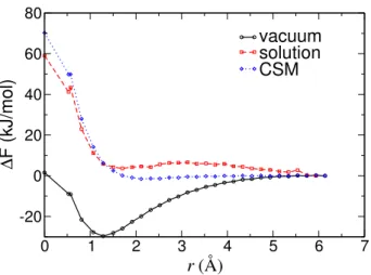
To study the solvation effects on the symmetric SN2 reaction we coupled the eDFT calculation above with an MDFT description of the SPC/E solvent. The electronic densities are computed for each geometry on a regular spatial grid made of 240⇥240⇥240 nodes. The same space grid is used for MDFT with 196 possible orientations. We choose the same set of Lennard-Jones parameters as the one used by Gao and Xia77 which are reminded in table 5. The eDFT and MDFT programs are run sequentially until a convergence criterion of 10 3 is reached for both the relative change in energy for GPAW and in free energy for MDFT. We apply the usual periodic boundary condition corrections of charged solutes83,84 and the correction due to the pressure overestimation in HNC85. The solvation free energy computed using eDFT/MDFT is displayed in figure 5. The minimum corresponding to the IDC almost vanished while the free energy barrier increases considerably to 58.7 kJ.mol 1. However, this value is still underestimated compared to the experimental value of 111 kJ.mol 186. The increase of the free energy barrier can be split into two contributions, the first one being the
polarisation of the solute by the solvent. It can be estimated by comparing the values of the in vacuo electronic functional evaluated with the equilibrium electronic densities obtained in vacuum and in the presence of the solvent. This polarisation contribution decreases the free energy barrier by 5.9 kJ.mol 1. The second and dominating contribution is the stabilisation by the solvent which increases the barrier by roughly 29 kJ.mol 1.
The solvation free energy profile was also computed using the CSM implemented in GPAW62, it is displayed in figure 5. The free energy barrier is 70.3 kJ.mol 1, a value that is also underestimated with respect to the experimental one.
The overall agreement of the eDFT/MDFT calculation may seem disappointing consid-ering that some previous studies were more quantitative, even with semi-empirical models78. However this work is the first attempt to self-consistently optimise molecular and electronic functionals. It is encouraging that the solvation effects are well reproduced, at least qualit-atively. Moreover, the free energy profile is consistent with the prediction of the CSM.
There are several avenues to improve the results, first the electronic functional is clearly not appropriate to reproduce the gas phase predictions, the MO6-2X functional87 seems more suited for instance39,49.
Second, the choice of the Lennard-Jones parameters may not be so innocent. This is particularly true in this SN2 reaction where the chlorine atom is described with the same parameters if it is bonded or in its anionic state. This seems to be natural in QM/MM studies, for instance in previous studies using the OPLS-AA force field the parameters for chlorine in halogenoalkane88 are used for all values of the reaction coordinate. It would probably be more correct to use a combination of the Lennard-Jones parameters of the chloride89 and the chlorine in halogenoalkane depending on the value of the reaction coordinate. From the MDFT point of view, we recover some known defects of the HNC functional and the SPC/E model, i.e. a missing bridge term for the former and no explicit treatment of water polarisability for the latter.
0 1 2 3 4 5 6 7 r (Å) -20 0 20 40 60 80 ∆ F (kJ/mol) vacuum solution CSM
Figure 5: Potential of mean force of the SN2 reaction as a function of the reaction coordin-ate. The calculation in vacuum is in full black and circles. The free energy in solution obtained with QM/MDFT is in dashed red with squares. The SFE obtained using the CSM implemented in GPAW is in dotted blue with diamonds.
Table 5: Lennard-Jones parameters for symmetrical SN2 reaction in water. (Å) ✏ (kJ.mol 1)
Cl 4.1964 0.4682 C 3.4000 0.4184 H 2.0000 0.29288
solvent structure at the molecular level. Indeed, the equilibrium density ⇢(r, ⌦) contains a lot of information about the solvation structure. In particular, it is possible to follow the solvent reorientation during the removal of the nucleofuge. To do so, we compute the average orientation density ¯⌦defined as
¯ ⌦(r) = R ⇢(r, ⌦)⌦d⌦ R ⇢(r, ⌦)d⌦ . (12)
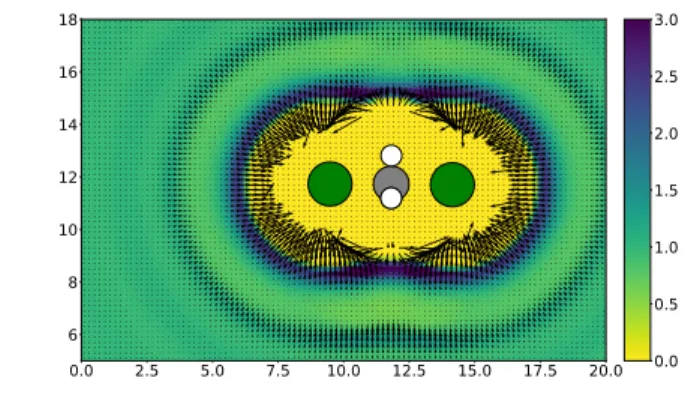
The direction of this vector gives the average orientation. Its norm gives the proportion of the average orientation with respect to other orientations. The average orientation density and the number density in a plane containing the carbon, the 2 chlorines and one hydrogen are displayed in figures 6-8 for the geometries of table 4. The average orientations are represented by vectors oriented from oxygen toward hydrogens which lengths are proportional to ¯⌦ . To improve the readability of the figure, orientation are depicted on a grid twice as loose as the one used for calculation.
Water number densities and average orientations around the TS are symmetrical with respect to the plane containing the CH3 fragment as displayed in figure 6. Concerning the number densities, we identify two high density shells separated by a region where the density is reduced compared to the bulk one. At every location in the second solvation shell the favoured orientations are the one with hydrogens pointing toward the solute. This is not surprising since the solute is globally negative, at this distance it is seen as a symmetric anion. However, other orientations are not insignificant as illustrated by the small size of the arrows. In the depletion region, there are no favoured orientations. In the first solvation shell, we first mention that the most marked orientations i.e the location denoted by the longest arrows are in the region the closest to the solute where the number density is almost zero. In this shell, the favoured orientations at any point are globally pointing toward the closest chlorine atom, except in a small region located close to the plane of the bisector of the Cl-Cl bond where the preferred orientations are pointing outward. Thus, the orientations in
the first solvation shell are consistent with the usual charge picture of the transition state in which each chlorine is globally anionic and the CH3 fragment is almost neutral39,49,78.
Figure 6: Average number density of water around the TS in the plane mentioned in the text. The high density region are in blue, the low density region are in yellow. The average orientation of the water molecule as computed by equation 12 are represented by arrows. Carbon atom is in grey, chlorine atoms are in green and hydrogen atoms are in white.
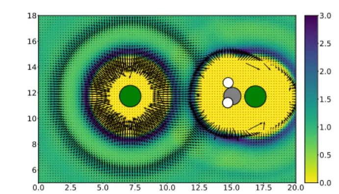
The number and average orientation densities around the structure corresponding to the IDC are displayed in figure 7. As compared to the TS, the number densities are not drastically modified. In the first solvation shell, the number density around the leaving chlorine is increased while the one around the bounded one is decreased. A similar effect is observed in the second solvation shell but it is less pronounced. The differences between the average orientation densities of the IC and the TS are more obvious. In the second solvation shell, the preferential orientations are still pointing toward the closest chlorine but the symmetry has clearly been broken. It looks like the superimposition of two spherical shells centred on each chlorine. The preferential orientations around the leaving chlorine are even more pronounced than in the TS while the one around the bounded one almost already recovered a bulk behaviour with no preferential orientations. A similar behaviour occurs in the first solvation shell which displays a decided average orientation around the leaving chlorine while the preferred orientations toward the bonded chlorine are still present but drastically reduced. These observations are consistent with an ionic complex. The two chlorines are anionic but the one the furthest from the carbon bears a more negative charge
than the closest one.
Figure 7: Same as figure 6 for the IDC.
In the dissociated state, displayed in figure 8, the number density and average orientation density follow a similar trend. The second shell around the chloromethane is no longer visible neither in number density nor in average orientation density. The two solvation shells around the leaving chlorine are spherical with a marked orientation pointing toward the nucleus which is consistent with an anion. The most interesting feature is observed in the first solvation shell of the chloromethane where the preferential orientations in the first solvation shell are pointing outward the molecule. This is quite surprising since in the usual point charges model where the chloromethane is described as a dipolar molecule, the water molecules close to chlorine would point toward this atom.
4 Conclusions
The introduced QM/MDFT approach is well suited to study solvation problems. It is particu-larly appropriate to compute solvation free energies and 3D molecular densities. QM/MDFT is based on the standard QM/MM approximation where the solute is described by quantum mechanics and solvent by molecular mechanics using ad hoc force fields. However, while the MM system is most often treated using Molecular Dynamics or Monte-Carlo we employ molecular density functional theory instead. It is no longer needed to generate extensive trajectory to compute free energy, this is the direct outcome of a much simpler functional minimisation. While any variational QM methods could be chosen in principle, electronic DFT is the most natural to be coupled with classical DFT33,34. With this choice, the solva-tion free energy can be computed doing a self-consistent optimisasolva-tion of the electronic and solvent functionals. This could be done simultaneously but the joint minimisation is done iteratively in this paper. This self-consistent approach accounts for the mutual polarisation of the solvent and solute, a phenomenon that is disregarded in previous attempt to couple eDFT and classical DFT38,39.
To illustrate the possibilities of QM/MDFT we first studied the solvation of a quantum water molecule in a solvent of classical water. The water dipole is enhanced in the liquid as compared to the gas phase. This is encouraging but the value of the dipole is underestimated with respect to the experimental measurement. Unfortunately, describing the solute at the QM level does not fix the known flaws of the MDFT functional at the HNC level, especially on the solvation structure. The first peak of the radial distribution between the oxygen of the solute and the oxygen of the solvent is too broad and the second peak is misplaced. This calls for bridge functional improvements that are currently underway.
We then turn to the study of a symmetrical aqueous SN2 reaction between chloromethane and chloride. The free energy profiles are qualitatively correct, the local minimum observed in gas phase vanished in the liquid. We were also able to follow in detail the solvation structure around the reactants along the reaction coordinate. However, the quantitative
agreement between the predicted solvation free energies and the experimental one is rather disappointing.
There are several rooms for improvement. First, the electronic functional should be carefully chosen as different functionals can predict energy barriers differing by several eV. Second, we should reexplore the corrections to the HNC molecular functional in the light of the QM/MM problem or better, complement the HNC functional by a well founded bridge term.
Another key point that must be addressed is the treatment of the repulsive and dispersion forces acting between the QM and the MM part. In this paper, we only dealt with the part of those forces that are generated by the QM solute and acts on the classical solvent. This was done by adding Lennard-Jones sites on the solute nuclei, as done in every QM/MM calculations. This is not completely satisfying because it alleviates the ab-initio nature of the method by adding arbitrary parameters. Besides, the reverse effect of the repulsive and dispersion forces created by the classical solvent and acting on the QM solute is currently neglected. They could be taken into account by adding an embedding potential into the QM calculation. Such embedding potential could be computed by using electron-solvent molecule pseudo-potentials52,54–56, or consistently within eDFT, by using an effective electron density of the solvent, obtained by "dressing up" the classical density with a frozen electronic density29,90. It could also prove necessary to employ an electronic functional that is able to describe the long-range dispersion interactions correctly91.
These points surely need to be explored to make the QM/MDFT method more robust to become a credible alternative to expansive AIMD or too simplistic continuum solvent models.
5 Acknowledgement
This work has been supported by the Agence Nationale de la Recherche, projet ANR BRIDGE AAP CE29.
References
(1) Hughes, E. D.; Ingold, C. K. 55. Mechanism of substitution at a saturated carbon atom. Part IV. A discussion of constitutional and solvent effects on the mechanism, kinetics, velocity, and orientation of substitution. J. Chem. Soc. 1935, 244–255.
(2) Liu, X.; Zhang, J.; Yang, L.; Hase, W. L. How a Solvent Molecule Affects Compet-ing Elimination and Substitution Dynamics. Insight into Mechanism Evolution with Increased Solvation. J. Am. Chem. Soc. 2018, 140, 10995–11005.
(3) Han, Y.; Jiang, D.; Zhang, J.; Li, W.; Gan, Z.; Gu, J. Development, applications and challenges of ReaxFF reactive force field in molecular simulations. Front. Chem. Sci. Eng. 2016, 10, 16–38.
(4) Senftle, T. P.; Hong, S.; Islam, M. M.; Kylasa, S. B.; Zheng, Y.; Shin, Y. K.; Junker-meier, C.; Engel-Herbert, R.; Janik, M. J.; Aktulga, H. M.; Verstraelen, T.; Grama, A.; van Duin, A. C. T. The ReaxFF reactive force-field: development, applications and future directions. Npj Comput. Mater. 2016, 2, 1–14.
(5) Frenkel, D.; Smit, B. Understanding molecular simulation: from algorithms to applica-tions, second edition ed.; Academic Press, 2002.
(6) Silvestrelli, P. L.; Parrinello, M. Water Molecule Dipole in the Gas and in the Liquid Phase. Phys. Rev. Lett. 1999, 82, 3308–3311.
(7) Lin, H.; Truhlar, D. G. QM/MM: what have we learned, where are we, and where do we go from here? Theor. Chem. Acc. 2007, 117, 185.
(8) Tomasi, J.; Persico, M. Molecular Interactions in Solution: An Overview of Methods Based on Continuous Distributions of the Solvent. Chem. Rev. 1994, 94, 2027–2094. (9) Tomasi, J.; Mennucci, B.; Cammi, R. Quantum Mechanical Continuum Solvation
Mod-els. Chem. Rev. 2005, 105, 2999–3094.
(10) Klamt, A. The COSMO and COSMO-RS solvation models. Wiley Interdiscip. Rev. Comput. Mol. Sci. 2011, 1, 699–709.
(11) Hansen, J.-P.; McDonald, I. Theory of Simple Liquids, Third Edition, 3rd ed.; Academic Press, 2006.
(12) Chandler, D.; Andersen, H. C. Optimized Cluster Expansions for Classical Fluids. II. Theory of Molecular Liquids. J. Chem. Phys. 1972, 57, 1930–1937.
(13) Ebner, C.; Saam, W. F.; Stroud, D. Density-functional theory of simple classical fluids. I. Surfaces. Phys. Rev. A 1976, 14, 2264–2273.
(14) Belloni, L.; Chikina, I. Efficient full Newton-Raphson technique for the solution of molecular integral equations - example of the SPC/E water-like system. Mol. Phys. 2014, 112, 1246–1256.
(15) Ramirez, R.; Gebauer, R.; Mareschal, M.; Borgis, D. Density functional theory of solva-tion in a polar solvent: Extracting the funcsolva-tional from homogeneous solvent simulasolva-tions. Phys. Rev. E 2002, 66, 031206–031206–8.
(16) Zhao, S.; Ramirez, R.; Vuilleumier, R.; Borgis, D. Molecular density functional theory of solvation: From polar solvents to water. J. Chem. Phys. 2011, 134, 194102.
(17) Jeanmairet, G.; Levesque, M.; Borgis, D. Molecular density functional theory of water describing hydrophobicity at short and long length scales. J. Chem. Phys. 2013, 139, 154101–1–154101–9.
(18) Jeanmairet, G.; Levesque, M.; Vuilleumier, R.; Borgis, D. Molecular Density Functional Theory of Water. J. Phys. Chem. Lett. 2013, 4, 619–624.
(19) Jeanmairet, G.; Levesque, M.; Sergiievskyi, V.; Borgis, D. Molecular density functional theory for water with liquid-gas coexistence and correct pressure. J. Chem. Phys. 2015, 142, 154112.
(20) Jeanmairet, G.; Levy, N.; Levesque, M.; Borgis, D. Molecular density functional theory of water including density-polarization coupling. J. Phys. Condens. Matter 2016, 28, 244005.
(21) Jeanmairet, G.; Rotenberg, B.; Borgis, D.; Salanne, M. Study of a water-graphene capacitor with molecular density functional theory. J. Chem. Phys. 2019, 151, 124111. (22) Jeanmairet, G.; Rotenberg, B.; Levesque, M.; Borgis, D.; Salanne, M. A molecular density functional theory approach to electron transfer reactions. Chem. Sci. 2019, 10, 2130–2143.
(23) Kovalenko, A.; Hirata, F. Three-dimensional density profiles of water in contact with a solute of arbitrary shape: a RISM approach. Chem. Phys. Lett. 1998, 290, 237–244. (24) Ding, L.; Levesque, M.; Borgis, D.; Belloni, L. Efficient molecular density functional
theory using generalized spherical harmonics expansions. J. Chem. Phys. 2017, 147, 094107.
(25) Ten-no, S.; Hirata, F.; Kato, S. A hybrid approach for the solvent effect on the electronic structure of a solute based on the RISM and Hartree-Fock equations. Chem. Phys. Lett. 1993, 214, 391–396.
(26) Naka, K.; Sato, H.; Morita, A.; Hirata, F.; Kato, S. RISM-SCF study of the free-energy profile of the Menshutkin-type reaction NH3+CH3Cl!NH3CH3++Cl in aqueous solu-tion. Theor. Chem. Acc. 1999, 102, 165–169.
(27) Sato, H.; Kovalenko, A.; Hirata, F. Self-consistent field, ab initio molecular orbital and three-dimensional reference interaction site model study for solvation effect on carbon monoxide in aqueous solution. J. Chem. Phys. 2000, 112, 9463–9468.
(28) Kasahara, K.; Sato, H. Solvation Structure of LiClO4/Ethylene Carbonate Solution near a Graphite Electrode in Lithium-ion Batteries: 3D-RISM Study. Chem. Lett. 2018, 47, 311–314.
(29) Kaminski, J. W.; Gusarov, S.; Wesolowski, T. A.; Kovalenko, A. Modeling Solvato-chromic Shifts Using the Orbital-Free Embedding Potential at Statistically Mechanic-ally Averaged Solvent Density. J. Phys. Chem. A 2010, 114, 6082–6096.
(30) Zhou, X.; Kaminski, J. W.; Wesolowski, T. A. Multi-scale modelling of solvatochromic shifts from frozen-density embedding theory with non-uniform continuum model of the solvent: the coumarin 153 case. Phys. Chem. Chem. Phys. 2011, 13, 10565–10576. (31) Gusarov, S.; Ziegler, T.; Kovalenko, A. Self-Consistent Combination of the
Three-Dimensional RISM Theory of Molecular Solvation with Analytical Gradients and the Amsterdam Density Functional Package. J. Phys. Chem. A 2006, 110, 6083–6090. (32) Casanova, D.; Gusarov, S.; Kovalenko, A.; Ziegler, T. Evaluation of the SCF
Combin-ation of KS-DFT and 3D-RISM-KH; SolvCombin-ation Effect on ConformCombin-ational Equilibria, Tautomerization Energies, and Activation Barriers. J. Chem. Theory Comput. 2007, 3, 458–476.
(33) Petrosyan, S. A.; Rigos, A. A.; Arias, T. A. Joint Density-Functional Theory: Ab Initio Study of Cr2O3 Surface Chemistry in Solution. J. Phys. Chem. B 2005, 109, 15436–15444.
(34) Petrosyan, S. A.; Briere, J.-F.; Roundy, D.; Arias, T. A. Joint density-functional theory for electronic structure of solvated systems. Phys. Rev. B 2007, 75, 205105.
(35) Sundararaman, R.; Letchworth-Weaver, K.; Schwarz, K. A.; Gunceler, D.; Ozhabes, Y.; Arias, T. JDFTx: software for joint density-functional theory. SoftwareX 2017, 6, 278– 284.
(36) Sundararaman, R.; Letchworth-Weaver, K.; Arias, T. A. A computationally efficacious free-energy functional for studies of inhomogeneous liquid water. J. Chem. Phys. 2012, 137, 044107.
(37) Sundararaman, R.; Arias, T. A. Efficient classical density-functional theories of rigid-molecular fluids and a simplified free energy functional for liquid water. Comput. Phys. Commun. 2014, 185, 818–825.
(38) Tang, W.; Cai, C.; Zhao, S.; Liu, H. Development of Reaction Density Functional Theory and Its Application to Glycine Tautomerization Reaction in Aqueous Solution. J. Phys. Chem. C 2018, 122, 20745–20754.
(39) Cai, C.; Tang, W.; Qiao, C.; Jiang, P.; Lu, C.; Zhao, S.; Liu, H. A reaction density functional theory study of the solvent effect in prototype S N 2 reactions in aqueous solution. Phys. Chem. Chem. Phys. 2019,
(40) Tang, W.; Zhao, J.; Jiang, P.; Xu, X.; Zhao, S.; Tong, Z. Solvent Effects on the Sym-metric and AsymSym-metric SN2 Reactions in Acetonitrile Solution: A Reaction Density Functional Theory Study. J. Phys. Chem. B 2020,
(41) Sigfridsson, E.; Ryde, U. Comparison of methods for deriving atomic charges from the electrostatic potential and moments. J. Comput. Chem. 1998, 19, 377–395.
(42) Marenich, A. V.; Jerome, S. V.; Cramer, C. J.; Truhlar, D. G. Charge Model 5: An Extension of Hirshfeld Population Analysis for the Accurate Description of Molecular Interactions in Gaseous and Condensed Phases. J. Chem. Theory Comput. 2012, 8, 527–541.
(43) Hu, H.; Lu, Z.; Yang, W. Fitting Molecular Electrostatic Potentials from Quantum Mechanical Calculations. J. Chem. Theory Comput. 2007, 3, 1004–1013.
(44) Borgis, D.; Gendre, L.; Ramirez, R. Molecular Density Functional Theory: Application to Solvation and Electron-Transfer Thermodynamics in Polar Solvents. J. Phys. Chem. B 2012, 116, 2504–2512.
(45) Evans, R. The nature of the liquid-vapour interface and other topics in the statistical mechanics of non-uniform, classical fluids. Adv. Phys. 1979, 28, 143.
(46) Levesque, M.; Marry, V.; Rotenberg, B.; Jeanmairet, G.; Vuilleumier, R.; Borgis, D. Solvation of complex surfaces via molecular density functional theory. J. Chem. Phys. 2012, 137, 224107–224107–8.
(47) Hohenberg, P.; Kohn, W. Inhomogeneous Electron Gas. Phys. Rev. 1964, 136, B864. (48) Sholl, D. S.; Steckel, J. A. Density Functional Theory: A Practical Introduction; John
Wiley & Sons, Inc., 2009.
(49) Tirado-Rives, J.; Jorgensen, W. L. QM/MM Calculations for the Cl- + CH3Cl SN2 Reaction in Water Using CM5 Charges and Density Functional Theory. J. Phys. Chem. A 2019, 123, 5713–5717.
(50) Riccardi, D.; Li, G.; Cui, Q. Importance of van der Waals Interactions in QM/MM Simulations. J. Phys. Chem. B 2004, 108, 6467–6478.
(51) Tu, Y.; Laaksonen, A. On the effect of Lennard-Jones parameters on the quantum mech-anical and molecular mechmech-anical coupling in a hybrid molecular dynamics simulation of liquid water. J. Chem. Phys. 1999, 111, 7519–7525.
(52) Vaidehi, N.; Wesolowski, T. A.; Warshel, A. Quantum-mechanical calculations of solva-tion free energies. A combined ab initio pseudopotential free-energy perturbasolva-tion
ap-(53) Schnitker, J.; Rossky, P. J. An electron-water pseudopotential for condensed phase simulation. J. Chem. Phys. 1987, 86, 3462–3470, Publisher: American Institute of Physics.
(54) Turi, L.; Gaigeot, M.-P.; Levy, N.; Borgis, D. Analytical investigations of an electron-water molecule pseudopotential. I. Exact calculations on a model system. J. Chem. Phys. 2001, 114, 7805–7815.
(55) Turi, L.; Borgis, D. Analytical investigations of an electron-water molecule pseudopo-tential. II. Development of a new pair potential and molecular dynamics simulations. J. Chem. Phys. 2002, 117, 6186–6195.
(56) Mones, L.; Turi, L. A new electron-methanol molecule pseudopotential and its applica-tion for the solvated electron in methanol. J. Chem. Phys. 2010, 132, 154507, Publisher: American Institute of Physics.
(57) Sifain, A. E.; Lubbers, N.; Nebgen, B. T.; Smith, J. S.; Lokhov, A. Y.; Isayev, O.; Roitberg, A. E.; Barros, K.; Tretiak, S. Discovering a Transferable Charge Assignment Model Using Machine Learning. J. Phys. Chem. Lett. 2018, 9, 4495–4501.
(58) Enkovaara, J.; Rostgaard, C.; Mortensen, J. J.; Chen, J.; Dułak, M.; Ferrighi, L.; Gavn-holt, J.; Glinsvad, C.; Haikola, V.; Hansen, H. A.; Kristoffersen, H. H.; Kuisma, M.; Larsen, A. H.; Lehtovaara, L.; Ljungberg, M.; Lopez-Acevedo, O.; Moses, P. G.; Ojanen, J.; Olsen, T.; Petzold, V.; Romero, N. A.; Stausholm-Møller, J.; Strange, M.; Tritsaris, G. A.; Vanin, M.; Walter, M.; Hammer, B.; Häkkinen, H.; Madsen, G. K. H.; Nieminen, R. M.; Nørskov, J. K.; Puska, M.; Rantala, T. T.; Schiøtz, J.; Thy-gesen, K. S.; Jacobsen, K. W. Electronic structure calculations with GPAW: a real-space implementation of the projector augmented-wave method. J. Phys. Condens. Matter 2010, 22, 253202.
Dułak, M.; Friis, J.; Groves, M. N.; Hammer, B.; Hargus, C.; Hermes, E. D.; Jen-nings, P. C.; Jensen, P. B.; Kermode, J.; Kitchin, J. R.; Kolsbjerg, E. L.; Kubal, J.; Kaasbjerg, K.; Lysgaard, S.; Maronsson, J. B.; Maxson, T.; Olsen, T.; Pastewka, L.; Peterson, A.; Rostgaard, C.; Schiøtz, J.; Schütt, O.; Strange, M.; Thygesen, K. S.; Vegge, T.; Vilhelmsen, L.; Walter, M.; Zeng, Z.; Jacobsen, K. W. The atomic simula-tion environment—a Python library for working with atoms. J. Phys. Condens. Matter 2017, 29, 273002.
(60) Mortensen, J. J.; Hansen, L. B.; Jacobsen, K. W. Real-space grid implementation of the projector augmented wave method. Phys. Rev. B 2005, 71, 035109.
(61) Ten-no, S.; Hirata, F.; Kato, S. Reference interaction site model self-consistent field study for solvation effect on carbonyl compounds in aqueous solution. J. Chem. Phys. 1994, 100, 7443–7453.
(62) Held, A.; Walter, M. Simplified continuum solvent model with a smooth cavity based on volumetric data. J. Chem. Phys. 2014, 141, 174108.
(63) Luukkonen, S.; Levesque, M.; Belloni, L.; Borgis, D. Hydration free energies and solva-tion structures with molecular density funcsolva-tional theory in the hypernetted chain ap-proximation. J. Chem. Phys. 2020, 152, 064110.
(64) Soper, A. K. The radial distribution functions of water and ice from 220 to 673 K and at pressures up to 400 MPa. Chem. Phys. 2000, 258, 121–137.
(65) Mark, P.; Nilsson, L. Structure and Dynamics of the TIP3P, SPC, and SPC/E Water Models at 298 K. J. Phys. Chem. A 2001, 105, 9954–9960.
(66) Clough, S. A.; Beers, Y.; Klein, G. P.; Rothman, L. S. Dipole moment of water from Stark measurements of H2O, HDO, and D2O. J. Chem. Phys. 1973, 59, 2254–2259.
(67) Gubskaya, A. V.; Kusalik, P. G. The total molecular dipole moment for liquid water. J. Chem. Phys. 2002, 117, 5290–5302.
(68) Badyal, Y. S.; Saboungi, M.-L.; Price, D. L.; Shastri, S. D.; Haeffner, D. R.; Soper, A. K. Electron distribution in water. J. Chem. Phys. 2000, 112, 9206–9208.
(69) Rocha, W. R.; Coutinho, K.; de Almeida, W. B.; Canuto, S. An efficient quantum mechanical/molecular mechanics Monte Carlo simulation of liquid water. Chem. Phys. Lett. 2001, 335, 127–133.
(70) Allesch, M.; Schwegler, E.; Gygi, F.; Galli, G. A first principles simulation of rigid water. J. Chem. Phys. 2004, 120, 5192–5198.
(71) McGrath, M. J.; Siepmann, J. I.; Kuo, I.-F. W.; Mundy, C. J. Spatial correlation of dipole fluctuations in liquid water. Mol. Phys. 2007, 105, 1411–1417.
(72) Gertner, B. J.; Wilson, K. R.; Hynes, J. T. Nonequilibrium solvation effects on reaction rates for model SN2 reactions in water. J. Chem. Phys. 1989, 90, 3537–3558.
(73) Ensing, B.; Meijer, E. J.; Blöchl, P. E.; Baerends, E. J. Solvation Effects on the SN2 Reaction between CH3Cl and Cl- in Water. J. Phys. Chem. A 2001, 105, 3300–3310. (74) Bento, A. P.; Solà, M.; Bickelhaupt, F. M. E2 and SN2 Reactions of X + CH3CH2X
(X = F, Cl); an ab Initio and DFT Benchmark Study. J. Chem. Theory Comput. 2008, 4, 929–940.
(75) Chandrasekhar, J.; Smith, S. F.; Jorgensen, W. L. SN2 reaction profiles in the gas phase and aqueous solution. J. Am. Chem. Soc. 1984, 106, 3049–3050.
(76) Chandrasekhar, J.; Smith, S. F.; Jorgensen, W. L. Theoretical examination of the SN2 reaction involving chloride ion and methyl chloride in the gas phase and aqueous solution. J. Am. Chem. Soc. 1985, 107, 154–163.
(77) Gao, J.; Xia, X. A two-dimensional energy surface for a type II SN2 reaction in aqueous solution. J. Am. Chem. Soc. 1993, 115, 9667–9675.
(78) Kuechler, E. R.; York, D. M. Quantum mechanical study of solvent effects in a prototype SN2 reaction in solution: Cl attack on CH3Cl. J. Chem. Phys. 2014, 140, 054109. (79) Zhao, Y.; Truhlar, D. G. Density Functional Calculations of E2 and SN2 Reactions:
Effects of the Choice of Density Functional, Basis Set, and Self-Consistent Iterations. J. Chem. Theory Comput. 2010, 6, 1104–1108.
(80) Huston, S. E.; Rossky, P. J.; Zichi, D. A. Hydration effects on SN2 reactions: an integral equation study of free energy surfaces and corrections to transition-state theory. J. Am. Chem. Soc. 1989, 111, 5680–5687.
(81) Barlow, S. E.; Van Doren, J. M.; Bierbaum, V. M. The gas phase displacement reaction of chloride ion with methyl chloride as a function of kinetic energy. J. Am. Chem. Soc. 1988, 110, 7240–7242.
(82) DePuy, C. H.; Gronert, S.; Mullin, A.; Bierbaum, V. M. Gas-phase SN2 and E2 reactions of alkyl halides. J. Am. Chem. Soc. 1990, 112, 8650–8655.
(83) Kastenholz, M. A.; Hünenberger, P. H. Computation of methodology-independent ionic solvation free energies from molecular simulations. I. The electrostatic potential in molecular liquids. J. Chem. Phys. 2006, 124, 124106.
(84) Kastenholz, M. A.; Hünenberger, P. H. Computation of methodology-independent ionic solvation free energies from molecular simulations. II. The hydration free energy of the sodium cation. J. Chem. Phys. 2006, 124, 224501.
(85) Sergiievskyi, V. P.; Jeanmairet, G.; Levesque, M.; Borgis, D. Fast Computation of Solvation Free Energies with Molecular Density Functional Theory: Thermodynamic-Ensemble Partial Molar Volume Corrections. J. Phys. Chem. Lett. 2014, 5, 1935–1942.
(86) Albery, W. J.; Kreevoy, M. M. In Adv. Phys. Org. Chem.; Gold, V., Bethell, D., Eds.; Academic Press, 1978; Vol. 16; pp 87–157.
(87) Zhao, Y.; Truhlar, D. G. The M06 suite of density functionals for main group ther-mochemistry, thermochemical kinetics, noncovalent interactions, excited states, and transition elements: two new functionals and systematic testing of four M06-class func-tionals and 12 other funcfunc-tionals. Theor. Chem. Acc. 2008, 120, 215–241.
(88) Jorgensen, W. L.; Schyman, P. Treatment of Halogen Bonding in the OPLS-AA Force Field: Application to Potent Anti-HIV Agents. J. Chem. Theory Comput. 2012, 8, 3895–3901.
(89) Jensen, K.; Jorgensen, W. Halide, ammonium, and alkali metal ion parameters for modeling aqueous solutions. J. Chem. Theory Comput. 2006, 2, 1499–1509.
(90) Wesolowski, T. A.; Shedge, S.; Zhou, X. Frozen-Density Embedding Strategy for Multi-level Simulations of Electronic Structure. Chem. Rev. 2015, 115, 5891–5928, Publisher: American Chemical Society.
(91) Grimme, S. Density functional theory with London dispersion corrections. Wires Com-put. Mol. Sci. 2011, 1, 211–228.


![[PDF] Tutoriel complet d’Introduction à Visual C# et Visual Studio 2008 | Formation informatique](data:image/gif;base64,R0lGODlhAQABAIAAAP///wAAACH5BAEAAAAALAAAAAABAAEAAAICRAEAOw==)