The Structured Way of Dealing with Heterogeneous Live Streaming Systems

HAL Id: hal-01538587

https://hal.inria.fr/hal-01538587

Submitted on 13 Jun 2017

HAL is a multi-disciplinary open access

archive for the deposit and dissemination of

sci-entific research documents, whether they are

pub-lished or not. The documents may come from

L’archive ouverte pluridisciplinaire HAL, est

destinée au dépôt et à la diffusion de documents

scientifiques de niveau recherche, publiés ou non,

émanant des établissements d’enseignement et de

Live Streaming Systems

Frédéric Giroire, Nicolas Huin, Andrea Tomassilli

To cite this version:

Frédéric Giroire, Nicolas Huin, Andrea Tomassilli. The Structured Way of Dealing with Heterogeneous

Live Streaming Systems. [Research Report] RR-9070, Inria Sophia Antipolis; Cnrs; Universite Cote

d’Azur. 2017, pp.25. �hal-01538587�

ISRN INRIA/RR--9070--FR+ENG

RESEARCH

REPORT

N° 9070

Dealing with

Heterogeneous Live

Streaming Systems

RESEARCH CENTRE

SOPHIA ANTIPOLIS – MÉDITERRANÉE

Frédéric Giroire, Nicolas Huin, Andrea Tomassilli

Project-Team Coati

Research Report n° 9070 — May 2017 — 22 pages

Abstract: Peer to peer networks are an efficient way to carry out video live streaming as the forwarding load is distributed among peers. These systems can be of two types: unstructured and structured. In unstructured overlays, the peers obtain the video in an opportunistic way. The advantage is that such systems handle well churn. However, they are less bandwidth efficient than structured overlays, the control overhead has a non-negligible impact on the performance. In structured overlays, the diffusion of the video is made via an explicit diffusion tree. The advantage is that the peer bandwidth can be optimally exploited. The drawback is that the departure of peers may break the diffusion tree.

In this work, we propose new simple distributed repair protocols for video live streaming structured systems. We show, through simulations with real traces, that structured systems can be very efficient and robust to failures, even for high churn and when peers have very heterogeneous upload bandwidth capabilities.

Key-words: peer-to-peer, video streaming, protocols, churn, reliability, diffusion tree, distributed algorithms

This work has been partially supported by ANR program Investments for the Future under reference ANR-11-LABX-0031-01.

Résumé : Les réseaux pair-à-pair sont un moyen efficace de diffuser des vidéos en direct. En effet, la charge en bande passante est répartie entre tous les pairs. Ces systèmes peuvent être de deux types: non structurés et structurés. Dans les systèmes non structurés, les pairs obtiennent la vidéo de manière opportuniste. L’avantage est que de tels systèmes gèrent bien le départ d’utilisateurs. Cependant, ils sont moins efficaces en bande passante, en raison des messages de contrôle et de la distribution opportuniste de la vidéo. Dans les systèmes structurés, la diffusion de la vidéo se fait via un arbre de diffusion explicite. L’avantage est que la bande passante peut être exploitée de manière optimale. L’inconvénient est que le départ de pairs risque de casser l’arbre de diffusion.

Dans ce travail, nous proposons de nouveaux protocoles simples distribués de réparation pour les systèmes structurés de diffusion vidéo en direct. Nous montrons, grâce à des simulations avec des traces réelles, que les systèmes structurés peuvent être très efficaces et robustes aux pannes, même pour un taux de churn élevé et lorsque les pairs possèdent des de bandes passantes très hétérogènes.

Mots-clés : pair-à-pair, diffusion video en direct, protocoles, fiabilité, arbre de diffusion, algorithmes distribués

Contents

1 Introduction 4

2 Related Works 4

3 Distributed Systems and Modeling 5

3.1 Modeling . . . 5

3.2 Metrics . . . 7

4 Protocols for Heterogeneous Systems 7 4.1 Description of the Protocols . . . 7

5 Simulations 9 5.1 Bandwidth Distributions . . . 9

5.2 Constant population . . . 10

5.3 Results with Twitch Traces . . . 14

5.4 Information update . . . 16

1

Introduction

In a live streaming scenario, a source streams a video to a set of clients, who want to watch it in real-time. Live streaming can be done either over a classic client-server architecture or over a distributed one. The high bandwidth required by a large number of clients watching the stream at the same time may saturate the source of a classic centralized architecture. In a distributed scenario (e.g., P2P), the bandwidth required can be spread among the users and the bottleneck at the source can be reduced. So, peer-to-peer systems are cheap to operate and scale well with respect to the centralized ones. Because of this, the P2P technology is an appealing paradigm for providing live streaming over the Internet.

In P2P context, two families of systems exist: structured or unstructured overlay networks. In structured overlay networks, peers are organized in a static structure with the source at the root of a diffusion tree. A node receives data from a parent node that can be a peer or the source of the stream. In unstructured overlay networks, peers self organize themselves without a defined topology. Unlike the structured case, a peer can receive each piece of the video from a different peer. The main challenge for P2P systems, compared to a classical multicast system, is to handle churn, that is the frequent arrival and departure of peers. In unstructured systems, the diffusion is done opportunistically and, as the authors show e.g. in [1], this ensures efficiency and robustness to the dynamicity of peers. Nevertheless, in this kind of systems, the control overhead may have a negative impact on the performance: network links and peer states need to be constantly monitored. In structured overlay, the content distribution is easier to manage. But, the departure of users may break the diffusion tree. Our goal is to too show, by proposing simple distributed repair mechanisms of the diffusion tree, that structured systems may be robust to churn, while keeping their advantages, an optimal diffusion rate and the continuity of diffusion. Contributions. In this work, we study a structured network for live video streaming experi-encing frequent node departures and arrivals in systems where nodes have heterogeneous upload bandwidth.

- We propose, in Section 4, simple distributed repair protocols to rebuild the diffusion tree, when peers are leaving. Different protocols use different levels of information.

- We compare the protocols using different metrics, i.e., delay, percentage of clients without video, number and duration of interruptions, see Section 5. We validate the protocols using different peer bandwidth distributions from literature.

- We study the efficiency of the protocols versus the level of information they use. We show that a repair protocol can be very efficient, even when using only a small amount of local information on its neighbors, see Sections 5.2.

- We use real Twitch traces to compare our different heterogeneous protocols in a real-life scenario of a streaming session in Section 5.3. We show that our simple distributed repair protocols work very well in practice.

- Finally, in Section 5.4 we compare the protocols in a setting where exact information is not always available.

2

Related Works

Structured vs unstructured systems. A general overview of P2P based live streaming services can be found in [2]. As stated, there are two main categories of distributed systems for

Variable Signification Default value n Number of nodes of the tree, root not included 1022

d Node bandwidth (or ideal node degree)

-h Height of the tree (root is at level 1)

-µ Repair rate (avg. operation time: 100 ms) 1 λ Individual churn rate (avg. time in the system: ₆₀₀₀1

10 min)

Λ System churn rate (Λ = λn) 1022₆₀₀₀ ≈ 0.17

Terminology Values

unit of time 100 ms

systems with low churn Λ ∈ [0, 0.4] systems with high churn Λ ∈ [0.4, 1]

Table 1: Summary of the main variables and terminologies used in this work.

video live streaming: unstructured and structured, even if hybrid solutions are also possible [3]. In unstructured overlay networks, peers self organize themselves in an overlay network, that does not have a defined topology. CoolStreaming/DONet [4] is an implementation of this approach. In structured overlay networks, peers are organized in a static structure with the source at the root of the tree. There are many techniques used in P2P live streaming with single-source and structured topology. These techniques may fall into two categories: single-tree and multiple-tree. In the single-tree approach each node is connected to a small number of nodes to which it is responsible for providing the data stream. ZIGZAG [5] is an example of this approach. In the multiple-tree approach the main idea is to stripe the content across a forest of multicast trees where each node is a leaf in every tree except one, as done by SplitStream [6].

Reliability In terms of reliability, unstructured systems are considered the best choice. As shown in [1] this kind of systems is able to handle churn (peers leaving the system) is a very efficient way. That is often explained by the complexity of making a structured system reliable. However, we show in this study that reliability can be ensured, for a simple system, efficiently by a simple algorithm.

In existing studies of structured systems, see e.g. [6, 7] and [8], authors focus on the feasibility, construction time and characteristics of the established overlay network. But these works usually do not consider over the issue of tree maintenance. Only few works focus on it. In [9] the authors propose a simple distributed repair algorithm that allows to fast recover and obtain a balanced tree after one or multiple failures. In [10] the authors develop a simple repair and distributed protocol based on a structured overlay network. By providing, through analysis and simulations, estimations of different system metrics like bandwidth usage, delay and number of interruptions of the streaming, they show that a structured live streaming systems can be very efficient and resistant to churn. However, their study is based on the fact that all nodes have the same bandwidth, where the bandwidth determines the maximum number of other nodes that can be served simultaneously. We extend their work to the case of peers with heterogeneous bandwidth.

3

Distributed Systems and Modeling

3.1

Modeling

We model a live streaming system as a tree of size n + 1 where the root represents a source streaming a live video. A summary of the variables used in this work is given in Table 1. The n

13 15 14 16 17 18

12

7

3

6

13 15 14 16

17 18

12

7

3

6

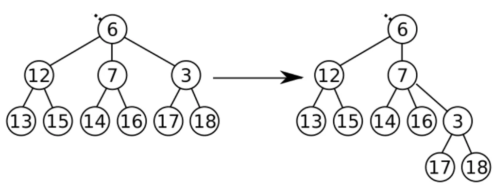
Figure 1: Example of a push operation carried out by the overloaded Node 6.

12 13 14 15

6

7

3

12 13

14 15

6

7

1

1

Figure 2: Example of the operation made after the departure of Node 3.

other nodes are clients wanting to watch the video. The source is the only reliable node of the network, all other peers may be subject to failure. A node v has a limited bandwidth d(v) used to serve its children. A node v is said to be overloaded, when it has more than d(v) children. In this case, it cannot serve all its children and some of them do not receive the video. Note that the delay between the broadcast of a piece of media by the source and the reception by a peer is given by its distance from the root in the logical tree. Hence our goal is to minimize the tree depth, while respecting degree constraints.

Each node applies the following algorithm with a limited knowledge of the whole network. - When a node is overloaded, it carries out a push operation. It selects two of its children,

and the first one is reattached to the second one, becoming a grandchild. Figure 1 presents an example of such operation.

- When a node leaves the system, one of its child is selected to replace him. The other children reattach to it. An example is given in Figure 2. In this work, we only consider single failure. But multiple failures could be handled by considering the great grandfather of a node or by reattaching to the root.

- When a new node arrives, it is attached to the root.

Churn. We model the system churn rate with a Poisson model of rate Λ. A node departure (also called churn event) occurs after an exponential time of parameter Λ, that is in average after a time 1/Λ. We note the individual failure rate λ = Λ/n. Authors in [11, 12] carried out a measurement campaign of a large-scale overlay for multimedia streaming, PPLive [13]. Among other statistics, the authors report that the median time a user stays in such a system is around 10 minutes. In this study, we use this value as the default value.

Repair rate. When a node has a push operation to carry out, it has first to change its children list, and then to contact its two children implicated in the operation so that they also change their neighborhoods (father, grandfather or children). This communication takes some amount of time, that can vary depending on the node to contact and congestion inside the network. To take into account this variation, we model the repair time as a random variable with exponential distribution of parameter µ. [14] reports that the communication time in a streaming system is in average 79 ms. Thus, we believe that assuming an average repair time of 100 ms is appropriate. Default values. In the following, for the ease of reading, we normalize the repair rate to 1. We call unit of time the average repair time, 100 ms. The normalized default churn rate, for an average stay of 10 minutes, λ is thus 1/6000 and the system churn rate is Λ = nλ ≈ 0.17. These default values are indicated as typical examples and are reported in Table 1, but, in our experiments, we present results for a range of values of Λ between 0 and 1. We talk of low churn systemsfor values of Λ below 0.4, and of high churn systems for values above 0.4.

3.2

Metrics

To evaluate the performance of the different protocols, we are interested by the following metrics. Number of people not receiving the video. Due to repairs and churn events, some people do not receive the video during small periods of time. We study what fraction of the nodes do not receive the video and during which amount of time.

Height of the tree or delay. The height of the diffusion tree gives the maximum delay between the source and a node.

Number of interruptions and interruption duration. We monitor the number of interrup-tions of the video diffusion to a node during the broadcast lifetime, as well as the distribution of interruptions duration.

4

Protocols for Heterogeneous Systems

We present three new repair protocols using different levels of knowledge. We then compare them, in particular to understand the trade-off between knowledge and performance.

4.1

Description of the Protocols

To obtain a tree with minimum height while respecting the degree constraints, the following two optimality conditionsmust hold:

1. If there exists a node at level L, all previous levels must be complete;

2. For each pair of levels (L, L + 1) the minimum bandwidth between all the nodes at level L must be greater than or equal to the maximum bandwidth between all the nodes at level L + 1.

Thus, the distributed protocols that we propose try to maintain nodes with high bandwidth on top of the diffusion tree. To this end, when a node is overloaded, it has to select carefully which node is pushed under which node using the information it has on the diffusion tree.

Local Bandwidth Protocol (LBP) In this protocol, each node knows the bandwidth of each of its children. Moreover, a node keeps track of the number of push operations done on each of its children. Note that this is a very local information that the protocol can easily get.

When a node is overloaded, it pushes its son with the smallest bandwidth, as nodes with higher bandwidth should stay on top on the diffusion tree. This son has to be pushed on a node

receiving the video. We consider all the nodes receiving the video and push on them proportion-ally to their bandwidth (e.g., a node with a bandwidth of d = 4 should receive twice as much pushes than a node with a bandwidth of d = 2). In details, the expected number of pushes to each son is proportional to its bandwidth. The father then pushes into the son with the largest difference between the push operations done and the expected number of push operations. Bandwidth Distribution Protocol (BDP) In this protocol, nodes have additional infor-mation. Each node knows the bandwidth of each of its children and the bandwidth distribution of the subtree rooted in each of its children. Note that the bandwidth distribution can be pulled up from the subtree. This may be consider costly by the system designer. However, it is also possible for a node to estimate this distribution by keeping the information of the bandwidth of the nodes pushed into it.

This additional information allows to estimate the optimal height of the subtrees of each of the sons. Thus, when a node is overloaded, it can push its son with the smallest bandwidth into its son (receiving the video) with the smallest estimated height.

Full Level Protocol (FLP) In this protocol, each node knows the bandwidth of each of its children and the last full level of the subtree rooted in each of its children.

This information allows to know in which subtree nodes are missing. The main idea is to push toward the first available slot in order to not increase the height of the diffusion tree. When a node is overloaded, its son with the smallest bandwidth is pushed into the son with the smallest last full level.

For all three protocols, a churn event is handled similarly. When a node leaves the system, the children of the falling node are adopted by their grandfather.

Discussion. In LBP, a node has no information about the underlying subtree. Push operations are carried out according to the degree of the nodes that receive the video. Since nodes may leave the system at any moment, it can thus happen that a node is pushed into the worst subtree. In BDP, a node knows the bandwidth distribution of each subtree rooted in each one of its children. A node is pushed according to the estimated height of the subtree rooted in its children. In the estimation a node assumes that all the levels, except the last one, is complete. Hence, it can happen that a node is not pushed on the best subtree.

In FLP, a node knows the last full level of the subtree rooted in each one of its children. A node is pushed under the node with the smallest value. In this way, we are sure that the node is pushed toward the best possible position. This may not be enough. In fact, due to nodes arrival and nodes departure the two optimality conditions may be broken.

Thus, in none of the protocols, the two optimality conditions are always true. However, the transmission delay is not the unique factor that determines the QoS for users. In fact, other factors like time to attach a new node, number and duration of interruptions are as important as the transmission delay. So, we decided to keep the protocols as simple as possible taking into consideration all metrics.

Handling Free Riders. Some nodes in the system can have no upload bandwidth and thus cannot distribute the video to anyone. They are called free riders. They may pose difficulties and calls for special treatment. First, an obvious observation is that protocols should not push nodes under a free rider. All our protocols prevent this. More problematic, in some situations, deadlocks may appear in which some nodes do not receive the video and all their brothers are free riders. The situation cannot be solved by push operations. In this case, we decided to ask the concerned free riders to rejoin the system. This is a solution we wanted to avoid as the goal of a structured protocol is to maintain as much as possible the parent-children relations of the diffusion tree. But, we considered that this is a small cost that free riders can pay, as they do not contribute to the system.

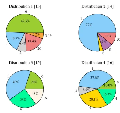
0 49.3% 1 18.7% 2 8.4% 20 18.4% 3-19 5.2%

Distribution 1 [13]

Distribution 2 [14]

Distribution 3 [15]

Distribution 4 [16]

Figure 3: Bandwidth distributions used in the simulations

5

Simulations

We study and compare the performance of the protocols for 4 bandwidth distributions of live video streaming systems that we found in the literature and that we present in Section 5.1. We first consider a scenario with a constant population to understand well the differences between the protocols in Section 5.2. We then use real traces of live streaming from Twitch in Section 5.3. Last, we discuss how to update in practice the information needed by the protocols in Section 5.4.

5.1

Bandwidth Distributions

In [15], the authors estimate the outgoing bandwidth that hosts in the live video streaming system can contribute. They use a combination of data mining, inference, and active measurements for the estimation. They set an absolute maximum bound of 20 for the out-degree. This means that each node can contributes for at most 20. In [16], the authors consider uplink rates from 256 kbps to 5 Mbps according to a distribution that reflects today’s different network access technologies. They assume an encoding rate of 250 kbps. The degree is then calculated as buplink(Kbps)/250c. In [17], the authors set the uploading bandwidths equal to 4000 kbps, 1000 kbps, 384 kbps, and 128 kbps corresponding to a distribution of 15%, 25%, 40%, and 20% of peers. We use as encoding rate 250 kbps and then calculate the outgoing degree as in the previous case. In [18] the authors, to come up with an accurate bandwidth distribution of Internet users, consider the measurement studies in [19] for the overall distribution of residential and Ethernet peers and [20] for the detailed bandwidth distribution of residential peers. As in the previous cases, we use 250 kbps as encoding rate to derive the degrees. The bandwidth distributions are summarized in Figure 3. In three of them (Distributions 1, 3 and 4), there is the presence of free riders, peers that join the system without sharing their own resources. We see that the peer

bandwidth can be very heterogeneous. For example, in Distribution 1, 49.3% of the peers are free riders, while 18.4% have bandwidth 20. Distributions 2 and 3 are similar (even if Distribution 2 has no free riders). The difference of degrees is smaller in Distribution 4. The fact that the degree distributions are pretty different allow us to test our algorithm for different settings.

5.2

Constant population

We compare the three protocols presented in the previous section according to four simple metrics: (i) average and maximum delay, (ii) percentage of people receiving the video, (iii) number of interruptions and (iv) their duration. We also add the Smallest Subtree Protocol (SSP) to the comparison, an optimal repair protocol for homogeneous systems proposed in [10]. We consider a range of churn rate between 0 and 1 on a system with 1022 clients for a duration of 30 000 unit of time. The population is constant in the system as we consider that when a node leaves the system, an other node rejoins at the root. The metrics are averaged over 30 experiments.

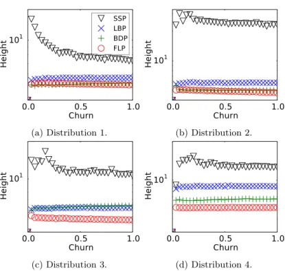
Height of the diffusion tree and delay. Figure 4 shows the average height (over time) of the diffusion tree as a function of the churn rate for the 4 bandwidth distributions. For all the distributions, SSP is the worst, by far, in terms of height and delay. Thus, SSP is not a good choice when peers have heterogeneous upload bandwidth capabilities. It is crucial to take the peer bandwidth into account and to try to place peers with high bandwidth on top of the diffusion tree, as we do in the three protocols proposed. For the 4 distributions, the average height of LBP is higher than the one of BDP which is higher than the one of FLP. They are respectively 5.5, 5.1, 5.1 for Distribution 1, 6, 5, 4.8 for Distribution 2, 6.2, 6, 5 for Distribution 3, 9.6, 7.6, and 7 for Distribution 4. Since the three protocols have the same behavior in the case of churn event, the explanation of the different behaviors relies on the different ways an overloaded node pushes a son. From the plots we can derive three main facts: (1) Homogeneous protocols are very inefficient for systems with heterogeneous upload bandwidth capabilities. (2) More information allows us to take better decisions. FLP is the best, followed by BDP and LBP (3) However, even with only very local information, we can have good results. In LBP, a node has access to a a very small amount of information about the underlying subtree and its performance is close to the one of FLP in which a node has more information about its subtree. Percentage of people without the video during time. Figure 5 shows the average per-centage of nodes which do not receive video as a function of the churn rate. As for the previous metric, SSP shows very bad results when peers have heterogeneous upload bandwidth capabil-ities. In fact, the percentage of people without video arrives to 70% for Distribution 1. On the other side, the three proposed protocols behave in a very similar and efficient way. The average percentage of peers without video for the three protocols LBP, BDP and FLP never exceeds 0.2%, if we consider systems with low churn (Λ ∈ [0, 0.4]), and 0.6%, if we consider systems

0.0 0.5 1.0 Churn 101 Height SSP LBP BDP FLP (a) Distribution 1. 0.0 0.5 1.0 Churn 101 Height (b) Distribution 2. 0.0 0.5 1.0 Churn 101 Height (c) Distribution 3. 0.0 0.5 1.0 Churn 101 Height (d) Distribution 4.

Figure 4: Average height of the diffusion tree as a function of the churn rate (1022 nodes).

0.0 0.5 1.0 Churn 0% 10% 20% 30% 40% 50% 60% 70% 80%

Peers w\o video

SSP LBP BDP FLP 0.0 0.5 1.0 Churn 0.0% 0.05% 0.1% 0.15% 0.2% 0.25% 0.3% 0.35%

Peers w\o video

(a) Distribution 1 0.0 0.5 1.0 Churn 0.0% 0.5% 1.0% 1.5% 2.0% 2.5% 3.0% 3.5% 4.0% 4.5%

Peers w\o video

SSP LBP BDP FLP 0.0 0.5 1.0 Churn 0.0% 0.05% 0.1% 0.15% 0.2% 0.25% 0.3% 0.35%

Peers w\o video

(b) Distribution 2 0.0 0.5 1.0 Churn 0% 10% 20% 30% 40% 50% 60%

Peers w\o video

SSP LBP BDP FLP 0.0 0.5 1.0 Churn 0.0% 0.05% 0.1% 0.15% 0.2% 0.25% 0.3% 0.35% 0.4%

Peers w\o video

(c) Distribution 3 0.0 0.5 1.0 Churn 0% 5% 10% 15% 20% 25% 30% 35%

Peers w\o video

SSP LBP BDP FLP 0.0 0.5 1.0 Churn 0.0% 0.1% 0.2% 0.3% 0.4% 0.5% 0.6%

Peers w\o video

(d) Distribution 4

Figure 5: Average fraction of peers not receiving the video as a function of the churn rate (1022 nodes). Right: Same plot withouth SSP protocol.

0.0 0.5 1.0 Churn 0 10 20 30 40 50 60 Number of Interruptions SSP LBP BDP FLP 0.0 0.5 1.0 Churn 0 10 20 30 40 50 60 Number of Interruptions (a) Distribution 1 0.0 0.5 1.0 Churn 0 10 20 30 40 50 60 Number of Interruptions SSP LBP BDP FLP 0.0 0.5 1.0 Churn 0 10 20 30 40 50 60 Number of Interruptions (b) Distribution 2 0.0 0.5 1.0 Churn 0 10 20 30 40 50 60 Number of Interruptions SSP LBP BDP FLP 0.0 0.5 1.0 Churn 0 10 20 30 40 50 60 Number of Interruptions (c) Distribution 3 0.0 0.5 1.0 Churn 0 10 20 30 40 50 60 Number of Interruptions SSP LBP BDP FLP 0.0 0.5 1.0 Churn 0 10 20 30 40 50 60 Number of Interruptions (d) Distribution 4

Figure 6: Average number of interruptions of the streaming per node as a function of the churn rate. Right: Same plot withouth SSP protocol.

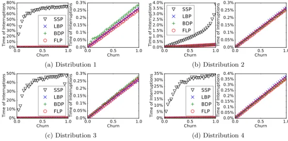
0.0 0.5 1.0 Churn 0% 10% 20% 30% 40% 50% 60% 70% 80% Time of Interruptions SSP LBP BDP FLP 0.0 0.5 1.0 Churn 0.0% 0.05% 0.1% 0.15% 0.2% 0.25% 0.3% Time of Interruptions (a) Distribution 1 0.0 0.5 1.0 Churn 0.0% 0.5% 1.0% 1.5% 2.0% 2.5% 3.0% 3.5% 4.0% Time of Interruptions SSP LBP BDP FLP 0.0 0.5 1.0 Churn 0.0% 0.05% 0.1% 0.15% 0.2% 0.25% 0.3% Time of Interruptions (b) Distribution 2 0.0 0.5 1.0 Churn 0% 10% 20% 30% 40% 50% Time of Interruptions SSP LBP BDP FLP 0.0 0.5 1.0 Churn 0.0% 0.05% 0.1% 0.15% 0.2% 0.25% 0.3% Time of Interruptions (c) Distribution 3 0.0 0.5 1.0 Churn 0% 5% 10% 15% 20% 25% 30% 35% Time of Interruptions SSP LBP BDP FLP 0.0 0.5 1.0 Churn 0.0% 0.05% 0.1% 0.15% 0.2% 0.25% 0.3% 0.35% 0.4% Time of Interruptions (d) Distribution 4

Figure 7: Average fraction of time for which the streaming as a function of the churn rate. Right: Same plot withouth SSP protocol.

(a) Distribution 1.

(b) Distribution 2.

(c) Distribution 3.

with high churn (Λ ∈ [0.4, 1]). The explanation of these similar behaviors is that a churn event is handled in the same way for the three protocols: the children of the peer, which leaves the system, are adopted by their grandfather.

Number and duration of interruptions. Figures 6 and 7 show respectively the average number of interruptions for a node present in the system during 30 000 units of time and the average fraction of time a node was interrupted. The tree protocols LBP, BDP and FLP have the same behavior. For the default value of churn rate, 0.17, measured on real PPLive [11], an average of 9 interruptions can be experienced for all the distributions.

This corresponds to an interruption every 3500 units of time (6 minutes). These interruptions have an imperceptible duration. In fact, for Λ = 0.17 in the worst case a node is interrupted in average for 0.05% of the time only. This corresponds to only 1.5 s. As discussed in the next section, with a very small buffer of few seconds of video, the users won’t experience any interruption. SSP exhibits a different behavior for this metric. For 3 of the 4 bandwidth distributions, it is the best protocols in terms of number of interruptions. However, the duration of these interruptions are much bigger. In fact, a peer may be interrupted even for the 75 % of the time for Distribution 1. The explanation of this behavior relies on the fact that, when a node in SSP is interrupted, it has to wait a high amount of time until it will start to see the video again. It is also explained by the lack of handling mechanism for free riders. This confirms that SSP should not be used in systems with heterogeneous peers. From now on, we will exclude SSP from our analysis and focus just on LBP, BDP and FLP.

Average depth for each value of bandwidth. Figure 8 shows the average depth (over time and over all nodes with the same bandwidth) for each bandwidth value as function of the churn rate. For all the distributions, nodes with the highest values of bandwidth are in the top layers of the tree and nodes with the smallest values of bandwidth are in the bottom positions of the tree. This leads to a better QoS for the peers sharing the most. These peers experience the smallest possible delay and the smallest number of interruptions among all the peers in the system. In fact, a peer is interrupted by the departure of one of its ancestors. Thus, peers in the top layers have a smaller probability of getting interrupted. On the other side, peers sharing less experience higher delay and, in average, a larger number of interruptions.

We can conclude that, for the three protocols LBP, BDP and FLP, the more a peer shares, the better its QoS is. A node has thus incentives to share its own resources and the protocols are robust to free riders.

5.3

Results with Twitch Traces

In order to simulate the protocols in real scenarios, we decided to use Twitch [21] as a Use Case. Twitch is a live streaming video platform that mainly focuses on video gaming and e-sport events. Twitch made its first appearance in 2011 and its popularity grew very fast. Today, with 1.5 million broadcasters and 100 millions visitors per month Twitch represents the 4th largest source of peak Internet traffic in the US [22]. With the goal of understanding the behavior of the viewers of the stream, we monitored the 100 most famous streamers (in terms of viewers and followers [23]).

We gathered the number of viewers for each moment of their streaming sessions. We noticed that most of the streaming sessions can be divided in 3 phases: (1) the start of the stream with a number of viewers increasing at an extremely high rate, (2) the central part of the stream with the number of viewers increasing at a slower rate than at the beginning of the stream and (3) the end of the stream with a decreasing number of viewers. See Figure 9 (Left)

Figure 9: Number of viewers as a function of the time for a streaming session of the user dizzykitten.

Phase 1

Phase 2

Phase 3

Arrival rate φ

0.0623196

0.0247548

0.0247548

Individual churn rate λ 1.572 ∗ 10

_{1.572 ∗ 10}

_{3.155 ∗ 10}

Duration (time units)

14640

112890

9648

Table 2: Parameters obtained from the model for the considered streaming session allows us to abstract from the real data and to repeat the simulations several time in order to estimate the quantitative behavior of the protocols more easily. Using the fact that, in average, a user spends 106 minutes on twitch.tv [24], for each phase, we calculate the arrival rate and the individual churn rate, modeled as a Poisson model. Table 2 shows the rates given to the simulator for the considered streaming session. In order to calculate the leaving rate of the 3rd phase, we assumed that the arrival rate of Phase 3 is the same as the one of Phase 2. Fig. 9 compares the data obtained from monitoring the user with the data obtained from the model.

We simulated our 3 protocols using the data generated from the model for our metrics of interest and according to the four distributions of bandwidth presented in the previous section. Table 3 summarizes the average results of the 3 protocols after 250 simulations.

Height of the diffusion tree and delay. We see that all protocols achieve a very small height of the diffusion tree: around 5 or 6 for the average. Recall that we have around 1500 users at the maximum of the stream. The protocols are thus very efficient. The evolution of the diffusion tree height is given as an example in Figure 10. We see the increase of height when the users connect to the stream till a maximum height of 6 for FLP and LBP, and of 7 for BDP. FLP for all the distributions gives us the tree with the smallest height. The results of LBP and BDP are different from the simulation case of previous section. In fact, since the individual churn rate is very small during the experiment (∼ 1.5 ∗ 10−5_{), pushing according to the children’s bandwidths}

(local information) reveals to be a good strategy, leading to a better height than BDP for 2 of the 4 distributions. In particular LBP behaves better than BDP in the case of very distant values of bandwidth (Distributions 1 and 3) and worst when the values of bandwidth are really close between them (Distribution 4).

Percentage of people without the video during time. In this case the 3 protocols behave similarly, as in the simulation case. They are very efficient: in average, only 0.2% of peers are

LBP BDP FLP

Height 5.66 6.1 5.17

People w/o video (%) 0.21 0.24 0.22 Number of Interruptions 17.54 12.12 20.87 Time of Interruptions (%) 0.01 0.01 0.017

(a) Distribution 1

LBP BDP FLP

Height 6.08 6.13 4.98

People w/o video (%) 0.21 0.21 0.22 Number of Interruptions 17.05 12.35 21.47 Time of Interruptions (%) 0.008 0.008 0.0013

(b) Distribution 2

LBP BDP FLP

Height 5.9 6.62 4.9

People w/o video (%) 0.21 0.21 0.22 Number of Interruptions 17.07 14.17 20.05 Time of Interruptions (%) 0.009 0.01 0.013

(c) Distribution 3

LBP BDP FLP

Height 9.12 7.9 7.06

People w/o video (%) 0.2 0.2 0.2

Number of Interruptions 5.62 5.57 6.76 Time of Interruptions (%) 0.009 0.008 0.009

(d) Distribution 4

Table 3: Average metrics after 250 simulations

Figure 10: Height of the diffusion tree during time for an example of Twitch session dizzykitten. unable to watch the video. Recall that we count the users arriving and waiting to be connected at the right place of the tree.

Number of interruptions during the diffusion. The protocols have a similar behavior in most cases. For Distributions 1, 2 and 3 the numbers of interruptions are between 12 and 21, for Distributions 4 is between 5 and 6. This means that, in the worst case, a peer staying for all the duration of the stream experiences an interruption every 10 minutes. In all cases the duration of these interruptions is very small. Considering all protocols and all the distributions, a node is never interrupted for more than the 0.02% of the time. This means, that a peer remaining during all the stream session is interrupted for less than 3 seconds. A buffer of few seconds (e.g. 10s) of video will make these interruptions imperceptible to the end-users. For a video rate of 480 kbps, it corresponds to a buffer size of only 40MB.

5.4

Information update

As we just showed in the last subsection, more information about the subtree leads to better repairs and thus to a better QoS for the clients. However, in order to maintain this information accurate, a node must exchange with all the nodes in its subtree. If the rate at which these

exchanges are done is too high, it can lead to message overhead and to a high delay from the moment a node joins the system until when the node starts to see the video. As a consequence, we tested the performance of FLP with the periodic update of the last full level information for a node. In the experiments we compare LBP with FLP protocol in the case a node obtains the exact last full level information after fixed time length intervals, expressed in time units.

0.0 0.5 1.0 Churn 4.0 4.2 4.4 4.6 4.8 5.0 5.2 5.4 5.6 5.8 Height 0.0 0.5 1.0 Churn 0.0% 0.05% 0.1% 0.15% 0.2% 0.25% 0.3% 0.35% 0.4%

Peers w\o video

LBP FLP 5 t.u. 10 t.u. 20 t.u. 40 t.u. 80 t.u. 100 t.u. 200 t.u. (a) Distribution 1 0.0 0.5 1.0 Churn 4.0 4.5 5.0 5.5 6.0 6.5 7.0 7.5 8.0 8.5 Height 0.0 0.5 1.0 Churn 0.0% 0.05% 0.1% 0.15% 0.2% 0.25% 0.3% 0.35%

Peers w\o video

LBP FLP 5 t.u. 10 t.u. 20 t.u. 40 t.u. 80 t.u. 100 t.u. 200 t.u. (b) Distribution 2 0.0 0.5 1.0 Churn 4.0 4.5 5.0 5.5 6.0 6.5 7.0 Height 0.0 0.5 1.0 Churn 0.0% 0.05% 0.1% 0.15% 0.2% 0.25% 0.3% 0.35% 0.4%

Peers w\o video

LBP FLP 5 t.u. 10 t.u. 20 t.u. 40 t.u. 80 t.u. 100 t.u. 200 t.u. (c) Distribution 3 0.0 0.5 1.0 Churn 5 6 7 8 9 10 11 Height 0.0 0.5 1.0 Churn 0.0% 0.1% 0.2% 0.3% 0.4% 0.5% 0.6%

Peers w\o video

LBP FLP 5 t.u. 10 t.u. 20 t.u. 40 t.u. 80 t.u. 100 t.u. 200 t.u. (d) Distribution 4

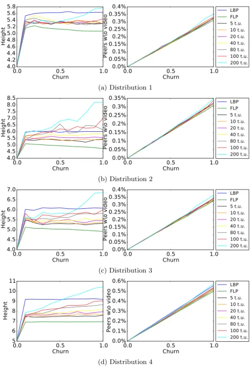
Figure 11: Average height of the tree (left) and percentage of people without video (right) as a function of the churn rate for LBP, FLP and FLP with periodic update of the last full level Impact of churn rate. Figure 11 shows the average height of the tree as a function of the churn rate for LBP, FLP and FLP with different update times. For low churn rates, the influence of the update time is barely noticeable. Introducing a delay of information only increases the average height of the tree of about half a level at most. As the churn increases, longest update time gives higher trees. However, even for high churn, FLP with update remains better than

LBP for intervals between update up to 100 t.u. (i.e., 10 s), except for Distribution 2. Having larger update times, e.g. 200 t.u., gives worst results than LBP for these churn values. This shows that FLP with periodic update should work well in practice, as the churn rate of practical systems is between 0.1 and 0.2, see the discution of Section 3.1. We confirm this in the following by consider Twitch streaming session.

FLP 100 200 300 400 500 600 700 800 900 1000 1100 LBP

Refresh Rate (time units)

5.1 5.2 5.3 5.4 5.5 5.6 5.7 Height (a) Distribution 1 FLP 100 200 300 400 500 600 700 800 900 1000 1100 LBP

Refresh Rate (time units)

4.5 5.0 5.5 6.0 6.5 7.0 7.5 Height (b) Distribution 2 FLP 100 200 300 400 500 600 700 800 900 1000 1100 LBP

Refresh Rate (time units)

4.8 5.0 5.2 5.4 5.6 5.8 6.0 6.2 6.4 Height (c) Distribution 3 FLP 100 200 300 400 500 600 700 800 900 1000 1100 LBP

Refresh Rate (time units)

6.5 7.0 7.5 8.0 8.5 9.0 9.5 Height (d) Distribution 4

Figure 12: Average height of the tree for LBP, FLP and FLP with periodic update of the last full levelfor the considered streaming session

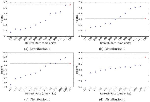
With Twitch streaming sessions. Figure 12 shows the average height of the tree during the streaming session for the protocols LBP, FLP and FLP with periodic update of the last full level. For Distribution 1, we see that FLP behaves better than LBP with refresh rates lower than 1100 units of time (corresponding to 1 min and 50 s). For Distribution 2, 3, and 4, the thresholds for the refresh rate respectively are 600 time units (1 min), 1 min and 20 s, and 2 min Such refresh rates correspond to only a few control messages around every minutes, which is negligible compared to the bandwidth used by the video streaming. This allows us to conclude that FLP can be used in real deployment, if we set a refresh rate according to the needs of the provider and to the arrival and churn rate of the peers in the stream. In fact, in this way, we can significantly reduce the overhead resulting from finding the last full level of the subtree at each iteration.

6

Conclusion

In this study we examined the problem of delivering live video streaming in a P2P overlay network using a structured overlay. We have proposed 3 distributed protocols to repair the diffusion tree

of the overlay, when there is churn. The protocols use different amounts of information. Using simulations and experiments with real traces from Twitch, we have shown that our protocols behave well with respect to fundamental QoS metrics, even for very heterogeneous bandwidth distributions. Our main result is that, with very simple distributed repair protocols using only a small amount of information, structured overlay networks can be very efficient and resistant to churn.

References

[1] T. Bonald, L. Massoulié, F. Mathieu, D. Perino, and A. Twigg, “Epidemic live streaming: optimal performance trade-offs,” in ACM SIGMETRICS Performance Evaluation Review, vol. 36, no. 1. ACM, 2008, pp. 325–336.

[2] B. Li, Z. Wang, J. Liu, and W. Zhu, “Two decades of internet video streaming: A retrospective view,” ACM Trans. Multimedia Comput. Commun. Appl., vol. 9, no. 1s, pp. 33:1–33:20, Oct. 2013. [Online]. Available: http://doi.acm.org/10.1145/2505805

[3] F. Wang, Y. Xiong, and J. Liu, “mtreebone: A hybrid tree/mesh overlay for application-layer live video multicast,” in 27th International Conference on Distributed Computing Systems (ICDCS’07). IEEE, 2007, pp. 49–49.

[4] X. Zhang, J. Liu, B. Li, and T. Yum, “Coolstreaming/donet: a data-driven overlay network for peer-to-peer live media streaming,” in INFOCOM 2005. 24th Annual Joint Conference of the IEEE Computer and Communications Societies. Proceedings IEEE, vol. 3, March 2005, pp. 2102–2111 vol. 3.

[5] D. Tran, K. Hua, and T. Do, “Zigzag: an efficient peer-to-peer scheme for media streaming,” in INFOCOM 2003. Twenty-Second Annual Joint Conference of the IEEE Computer and Communications. IEEE Societies, vol. 2, March 2003, pp. 1283–1292 vol.2.

[6] M. Castro, P. Druschel, A.-M. Kermarrec, A. Nandi, A. Rowstron, and A. Singh, “Split-stream: high-bandwidth multicast in cooperative environments,” in ACM SIGOPS Operat-ing Systems Review, vol. 37, no. 5. ACM, 2003, pp. 298–313.

[7] V. Venkataraman, K. Yoshida, and P. Francis, “Chunkyspread: Heterogeneous unstructured tree-based peer-to-peer multicast,” in 14th IEEE International Conference on Network Pro-tocols, 2006, pp. 2–11.

[8] G. Dan, V. Fodor, and I. Chatzidrossos, “On the performance of multiple-tree-based peer-to-peer live streaming,” in 26th IEEE International Conference on Computer Communications, 2007, pp. 2556–2560.

[9] F. Giroire, R. Modrzejewski, N. Nisse, and S. Pérennes, “Maintaining balanced trees for structured distributed streaming systems,” in International Colloquium on Structural Infor-mation and Communication Complexity. Springer, 2013, pp. 177–188.

[10] F. Giroire and N. Huin, “Study of Repair Protocols for Live Video Streaming Distributed Systems,” in IEEE GLOBECOM 2015 - Global Communications Conference, San Diego, United States, Dec. 2015. [Online]. Available: https://hal.inria.fr/hal-01221319

[11] X. Hei, C. Liang, J. Liang et al., “Insights into PPLive: A Measurement Study of a Large-Scale P2P IPTV System,” in International Word Wide Web Conference. IPTV Workshop, 2006.

[12] L. Vu, I. Gupta, J. Liang, and K. Nahrstedt, “Measurement of a large-scale overlay for multi-media streaming,” in Proceedings of the 16th international symposium on High performance distributed computing. ACM, 2007, pp. 241–242.

[14] B. Li, Y. Qu, Y. Keung, S. Xie, C. Lin, J. Liu, and X. Zhang, “Inside the new coolstream-ing: Principles, measurements and performance implications,” in 27th IEEE International Conference on Computer Communications, 2008.

[15] K. Sripanidkulchai, A. Ganjam, B. Maggs, and H. Zhang, “The feasibility of supporting large-scale live streaming applications with dynamic application end-points,” ACM SIG-COMM Computer Communication Review, vol. 34, no. 4, pp. 107–120, 2004.

[16] E. Setton, J. Noh, and B. Girod, “Low latency video streaming over peer-to-peer networks,” in 2006 IEEE International Conference on Multimedia and Expo, July 2006, pp. 569–572. [17] N. Efthymiopoulos, A. Christakidis, S. Denazis, and O. Koufopavlou,

“Liquid-stream—network dependent dynamic p2p live streaming,” Peer-to-Peer Networking and Applications, vol. 4, no. 1, pp. 50–62, 2011.

[18] Z. Liu, Y. Shen, K. W. Ross, S. S. Panwar, and Y. Wang, “Substream trading: towards an open p2p live streaming system,” in Network Protocols, 2008. ICNP 2008. IEEE Interna-tional Conference on. IEEE, 2008, pp. 94–103.

[19] M. Dischinger, A. Haeberlen, K. P. Gummadi, and S. Saroiu, “Characterizing residential broadband networks,” in Internet Measurement Comference, 2007, pp. 43–56.

[20] C. Huang, J. Li, and K. W. Ross, “Can internet video-on-demand be profitable?” ACM SIGCOMM Computer Communication Review, vol. 37, no. 4, pp. 133–144, 2007.

[21] “Twitch homepage, http://www.twitch.com/.”

[22] D. MacMillan and G. Bensinger, “Amazon to buy video site twitch for $970 million,” August 2014. [Online]. Available: http://www.wsj.com/articles/ amazon-to-buy-video-site-twitch-for-more-than-1-billion-1408988885

[23] “Twitch Statistics, http://socialblade.com/twitch/.”

[24] “Twitch Blog, https://blog.twitch.tv/twitch-hits-one-million-monthly-active-broadcasters-21dd72942b32.”