HAL Id: cea-02506820
https://hal-cea.archives-ouvertes.fr/cea-02506820
Submitted on 12 Mar 2020
HAL is a multi-disciplinary open access
archive for the deposit and dissemination of
sci-entific research documents, whether they are
pub-lished or not. The documents may come from
teaching and research institutions in France or
abroad, or from public or private research centers.
L’archive ouverte pluridisciplinaire HAL, est
destinée au dépôt et à la diffusion de documents
scientifiques de niveau recherche, publiés ou non,
émanant des établissements d’enseignement et de
recherche français ou étrangers, des laboratoires
publics ou privés.
L. Goldsteins, L. Buligins, Y. Fautrelle, C. Biscarrat, E. Platacis
To cite this version:
L. Goldsteins, L. Buligins, Y. Fautrelle, C. Biscarrat, E. Platacis. MHD instability analysis of a large
scale electromagnetic pump for pemdyn facility.. ICAPP 2015 - International Congress on Advances
in Nuclear Power Plants, May 2015, Nice, France. �cea-02506820�
MHD INSTABILITY ANALYSIS OF A LARGE SCALE ELECTROMAGNETIC PUMP FOR
PEMDYN FACILITY.
Goldsteins L.1,2,3, Buligins L. 2, Fautrelle Y. 3, Biscarrat C. 1, Platacis E. 4
1 CEA, CADARACHE, DTN/STPA/LCIT,
2
Faculty of Physics and Mathematics, University of Latvia,
3 Grenoble INP, SIMAP/EPM Laboratory,
4 Institute of Physics University of Latvia,
1
Bat.204, 13108 St Paul lès Durance, Cedex France
2 8 Zellu str., LV-1002, Riga, Latvia
3 Domaine Universitaire, BP 38402, Saint Martin d’Hères, Cedex France
4
32 Miera str., LV-2169, Salaspils, Latvia Email: [email protected]
Abstract – This paper focuses on numerical and experimental investigation of
magnetohydrodynamic (MHD) instability which can occur in an electromagnetic induction pump
(EMIP) in regimes when slip Magnetic Reynolds number (Rms) is sufficiently high. It has been
reported that MHD instability produces strong non-homogeneity of flow, low frequency pressure pulsations, vibrations and drop of developed pressure therefore it should be regarded as highly unwanted phenomenon. Detailed studies of this problem must be carried out to develop better understanding about working regimes and master control of EMIP.
I. INTRODUCTION
Large scale induction electromagnetic induction pumps (EMIP) are foreseen to be used in ASTRID (Advanced Sodium Technological Reactor for Industrial Demonstration) prototype1,2. A model facility is being built in CEA Cadarache called PEMDYN3 to investigate working regimes and master the control of annular linear induction pumps (ALIP). The launch of PEMDYN facility is expected in 2015.
There are number of investigations devoted to the development of ALIP. The instability criterion has been theoretically derived by Gailitis et al.0, the boundary between flow stability and instability has been determined experimentally in work of Ota et al.5, experimental and numerical results are compared by Araseki et al.6 While qualitative agreement between theoretical predictions and experiment can be observed, a more detailed analytical study (Goldsteins et al.7) and experiment with controlled velocity/magnetic field perturbation implementation is necessary to deepen the understanding of the instability mechanisms in EMIP. Also improved numerical models capable predicting MHD instability are necessary.
In support of activities in PEMDYN facility collaboration between CEA, University of Latvia (UL) and Institute of Physics of University of Latvia (IPUL) has
been launched for experimental studies of flat EMIP. The goal of these studies is to improve experimental investigation methods and provide reliable data for verification of numerical models.
In this paper main activities on MHD instability investigation are summarized as well as used numerical and experimental methods are conceptualized and principal results presented.
II. PEMDYN FACILITY
This large scale facility in CEA Cadarache is meant to model 1:2 scaled down ALIP similar to be used in ASTRID. The loop consists of the pump, three heat exchangers, a flow meter, valve, expansion tank and sodium supply tanks (fig. 1). In parallel sodium purification system will be installed to the loop.
Main characteristics of PEMDYN facility are:
Sodium flowrate up to 1450 m3/s
Hydraulic diameter of the channel 0.1m
Velocity in channel around 10 m/s
Na temperature 115 – 200° C
Bi-directional pumping
Fig. 1. A drawing of the PEMDYN facility.
There are totally 36 instrumentation mounting places in the inlet and outlet of the ALIP. The design of the PEMDYN pump allows changing passive ferromagnetic core with internal inductor or specially equipped core for measurements inside the ALIP.
The main task of PEMDYN facility is to master control of the ALIP in different scenarios of operation in nuclear power plant. This includes not only determining optimal operating parameters such as frequency, supply voltage etc., but also finding the threshold of stability, characterize stable/instable regimes and investigate in details mechanism of MHD instability formation using mainly experimental and numerical methods.
III. 2D NUMERICAL MODELS
MHD instability in ALIP is non-axysimmetric phenomena0,6,7,8; therefore appropriate numerical models are necessary. One of such models by Araseki6 can be found in literature where authors analyze rather detailed model of ALIP. The transient problem is solved in Θ-z coordinate system using in-house code. The induction equation is solved regarding induced magnetic field (only radial component considered) and Navier – Stokes equation considering Θ and z velocity components. Numerical results are compared with the experiment and although it is shown that used approach is capable of predicting MHD instability, authors admit that model is of qualitative nature.
To verify numerical model, first of all, it is necessary to test it on a basic case study which has an analytical solution. Model of real ALIP has too many higher order effects which cannot be described in a simple way, therefore analysis of a real pump can be done only afterwards.
However, another problem exists. The theory has not significantly improved since 70ies and in-depth studies on this topic have been restarted only lately7 and are still on-going. Nevertheless, from these theoretical results it is possible to calculate threshold of convective instability and
perturbation development rates which afterwards can be compared with numerical results of a test case.
Similar 2D models used by Araseki can be created using ANSYS FLUENT MHD module and are shown in this work. The advantages of such approach is that not only simple 2D cases can be studied, but also models can be rather easily upgraded to 3D, taking into account two component magnetic field, turbulent flow etc. However, computational costs in such case will be very high, since good spatial and temporal discretization is required.
In presented work 2D models with two component flow (y, z) and single component magnetic field (x) are studied. No special turbulence models were used; however viscose and turbulent dissipation is modeled using Darcy-Weisbach equation and Blasius approximation for friction factor. Induction equation is solved only for out of plane (Bx) component regarding induced magnetic field. The typical cell size of meshes is Δx = 3 mm, time step Δt = 10 -4 s and velocity 5 m/s. All residuals are set up to 10-5 and calculation time is from 0 – 1s.
III.A. 2D non-axysimmetrical model of infinite ALIP
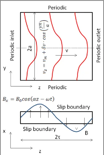
To study 2D radially averaged infinite ALIP following model in fig. 2 was created.
The geometry is a single wavelength long (2τ), consisting of two periodic conditions over y, which describes azimuthally continuity and periodic inlet and outlet over z, which describes infinite length over z axis. There is a single cell over x axis with slip condition on boundaries.
The model is initialized with 0.5% velocity z component perturbation (see fig. 2) from the mean flow before starting transient calculation. Cutting line over z is defined in the centre of the model. Then development of velocity perturbation amplitude averaged over the line in the center of the channel is registered.
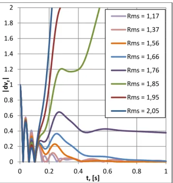
In (fig. 3.) results of normalized velocity perturbation modulus temporal development are presented. One can notice that there is certain development period (up to 0.25s) which is necessary to form perturbation amplitude of both field (initially only velocity field is perturbated). Afterwards one can observe that perturbation is either growing or either dying with a certain rate. It can be observed that critical Rms ≈ 1.8 which is significantly higher than expected from analytical estimations0: Rms ≈ 1.27.
Because causes of such result are not completely clear, detailed numerical studies should be carried out to estimate convective stability threshold more precisely not only by improving numerical model by itself but estimate influence of e.g. interaction parameter (N) on the result8.
Fig. 3. Temporal development of vz perturbation with Rm ≈ 6.44, N ≈ 10 and different Rms.
In (fig. 4) development of integral force over whole geometry is shown. As model is periodic, there are no double supply frequency (DSF) pulsations and it can be
observed that quasi – stationary regime is obtained after sufficient calculation time (~0.4s) in case of comparatively low Rms (1.17 – 1.76). Though curve (fig. 4. Rms = 1.85)
seems to be also “stable” this is not quite true, since perturbation is growing (see fig. 3). Actually perturbation has not increased enough to significantly disturb the flow (at 1s it is ~ 5% from mean flow). For comparatively high
Rms (1.95 and 2.05) perturbation has increased
significantly over 1s to seriously influence developed force (Rms = 1.95 at 0.9s and Rms = 2.05 at 0.7s perturbation is
~40 - 50% from mean flow).
Fig. 4. Transient development of integral axial force Fz with different Rms.
This result might give an idea about the limit of perturbation amplitude, which could be considered “low” and doesn’t significantly decrease performance of the EMIP. In fig. 4 can be observed that uncontrolled growth of perturbation may lead to significant loss of developed force (pressure) (Rms = 2.05).
This model could be also useful to analyze low frequency (LF) pulsations, which are directly connected with instability phenomenon. Since DSF pulsations does not appear in integral force characteristic, only LF can be observed (fig. 4. Rms = 2.05) and are easier to analyze.
Also much longer calculations are necessary (up to 10s), however, this might not be so time consuming as full model of the pump since only a single wavelength of EMIP is modelled. 0 0.2 0.4 0.6 0.8 1 1.2 1.4 1.6 1.8 2 0 0.2 0.4 0.6 0.8 1 |d vz | t, [s] Rms = 1,17 Rms = 1,37 Rms = 1,56 Rms = 1,66 Rms = 1,76 Rms = 1,85 Rms = 1,95 Rms = 2,05 0 2000 4000 6000 8000 10000 12000 0.0 0.2 0.4 0.6 0.8 1.0 Fz, [ N ] t, [s] Rms = 2,05 Rms = 1,95 Rms = 1,85 Rms = 1,76 Rms = 1,66 Rms = 1,56 Rms = 1,37 Rms = 1,17
III.B. 2D model of flat EMIP in TESLA-EMP facility
To compare numerical results with experimental data a finite length model of flat EMIP was created using practically the same methods as described in previous chapter.
Studied geometry is shown in fig. 5. It is a simplification of a real flat EMIP in TESLA-EMP (Test and Experimental Sodium Loop for Analysis of ElectroMagnetic Pumps) facility in IPUL described in the following chapter. It consists of inlet and outlet regions both 400 mm and active part with 1100 mm of length which is divided into 4 sub-channels. The total width of the geometry is 420 mm including thickness of stainless steel walls 4 mm and width of sub-channel 100mm. Height of the channel is 20 mm.
Fig. 5. Geometry of the EMIP model of TESLA-EMP.
Fig. 6. COMSOL and analytical fit of the external magnetic field Be x component in the middle of the channel.
External magnetic field is applied in 1500 mm long central part of geometry using analytical solution of an 2D infinite problem with discrete 3 phase current sources in
form of Fourier series. Only first four significant harmonics are considered. For applied field to be as precise as possible, amplitudes of each harmonic are fitted with numerical solution of COMSOL software which calculates the exact 2D geometry of inductor. Decay of the field outside the inductor is approximated with exponential functions. When good approximation is obtained through the height of the gap (fig. 6.), analytical solution of external field is height averaged and then applied to ANSYS FLUENT MHD module. Frequency of magnetic field is 50 Hz, which corresponds to the experiment.
In fig. 7 distribution of magnetic field is shown in the case of global flowrate Q = 45 l/s and effective current in the inductor I = 200A. Higher harmonics of the field are due to particular construction of inductor consisting of teeth and slots.
Fig. 7. Magnetic field (Bx) distribution: Q=45 l/s, I=200 A.
It can be observed that total magnetic field is somewhat stronger in side part (Channel-2) than in central part (Channel-1). Plot of distribution of the field is shown in fig. 8 where mentioned difference is more obvious.
Fig. 8. Magnetic field distribution in the middle of the channel. Red: channel-1, blue: channel-2.
-0.15 -0.1 -0.05 0 0.05 0.1 0.15 0 0.3 0.6 0.9 1.2 1.5 B ex , [T] z, [m] ANALITICAL FIT COMSOL -0.1 -0.08 -0.06 -0.04 -0.02 0 0.02 0.04 0.06 0.08 0.1 -0.1 0.2 0.5 0.8 1.1 1.4 1.7 Bx , [T] z, [m]
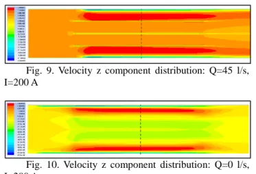
In fig. 9 and fig. 10 distribution of z velocity component is shown in cases of global flowrate Q = 45 l/s and Q = 0 l/s accordingly and effective current 200A.
Fig. 9. Velocity z component distribution: Q=45 l/s, I=200 A
Fig. 10. Velocity z component distribution: Q=0 l/s, I=200 A
It can be observed that in both cases velocity is higher in side sub-channels. Such effect has been already reported in experimental works with flat EMIPs operating with high slips magnetic Reynolds number9. In short it can be explained by fact that magnetic field is stronger in the side part of the channel and since force is proportional to field in second power, thus the higher velocity.
Moreover, in case of low flowrate velocity in central channels can be negative. Therefore highly inhomogeneous velocity distribution exists over width of the entire channel.
One should also note that there is a rather strong reversed flow near the outer wall of the channel (fig. 9 and fig. 10). Such effect appears due to the induced eddy currents which have to close and make a loop near the wall. Therefore the EM force is not that high any more in z direction and this recirculation region appears.
In fig. 11 distribution of z velocity component over width in the center of the channel is shown. It can be observed that not only velocity in both side and central channel increases flowrate but the difference between them becomes smaller.
Finally, velocity from fig. 11 and magnetic field amplitude from fig. 8. (transformed in form of voltage corresponding to sensitivity of sensor used in the experiment for easier comparison) in the canter of channel-1 and -2 are compared in fig. 12 and fig. 13.
Fig. 11.Velocity z component distribution over y axis in the middle of the EMIP as a function of flowrate.
Fig. 12. Velocity of in the center of channel-1 and calculated voltage corresponding to magnetic field maximum. -8 -6 -4 -2 0 2 4 6 8 -0.21 -0.14 -0.07 0 0.07 0.14 0.21 Vz , [ m /s] y, [m] Q = 0 [L/s] Q = 10 [L/s] Q = 20 [L/s] Q = 30 [L/s] Q = 45 [L/s] 0.5 0.52 0.54 0.56 0.58 0.6 0.62 0.64 -2 -1 0 1 2 3 4 5 6 0 10 20 30 40 50 U, [ V] Vz , [ m /s] Q, [L/s] Vz, Channel-1 UX-1, V
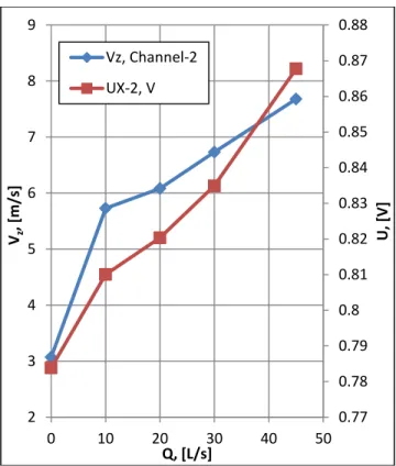
Fig. 13. Velocity of in the center of channel-2 and calculated voltage corresponding to magnetic field maximum.
By analyzing figures above one can notice, that voltage (magnetic field amplitude) increases with velocity. Also in channel-1 were overall lower velocities are observed overall voltage is also lower if compared to channel-2. Moreover, velocity changes from -1.5 up to 5.5 m/s in channel-1 and increment of voltage is roughly 0.12V. In channel-2 velocity increases from 3 up to 7.7 m/s and increase of voltage is 0.08V.
One can also observe that there is a certain correlation between these two parameters. According to theory0 they are linked with relationship:
(1)
In the case of high magnetic Reynolds number and velocity of liquid metal low compared to synchronous velocity of magnetic field, one can write linear relationship:
(2) Therefore changes in magnetic field amplitude should be an indication of changes in the velocity distribution. Since measurement of magnetic field is significantly easier than velocity measurement in liquid Na this technique is used in experimental setup described in the next chapter.
IV. TESLA-EMP FACILITY
In collaboration of CEA and IPUL a set of three experiments on investigation of the stability of the EMIP are foreseen in a TESLA-EMP facility in IPUL. Principal scheme of the measuring and control system of the loop is shown in fig.14 and an overview in fig. 15.
Fig. 14. The principal scheme of the measuring and control system of TESLA-EMP facility
Fig. 15. The view of TESLA-EMP facility 0.77 0.78 0.79 0.8 0.81 0.82 0.83 0.84 0.85 0.86 0.87 0.88 2 3 4 5 6 7 8 9 0 10 20 30 40 50 U, [ V] Vz , [ m /s] Q, [L/s] Vz, Channel-2 UX-2, V
The loop can be equipped with two electromagnetic switchable induction pumps in parallel or in series theoretically providing a liquid metal flow rate up to 150 l/sat discharge pressure of 4.4 bars. Pressure measurements are performed using high temperature piezo-electric manometers with stainless steel membrane in the inlet and outlet of the pump. For flowrate measurements a Venturi tube is installed on the loop using same type of manometers. The working temperature of the loop is 200° C - 500° C. To control the temperature of the loop, it is equipped with three component (LM-Oil-H2O) heat exchanger with maximum cooling power 120 kW. The cooling power is controlled by the oil level in the ring-like channel. The control range is 2-120 kW at sodium temperature of 300° C.
The channel of the EMIP is equipped with magnetic field and temperature sensors. Up to 144 magnetic coils are foreseen to determine the distribution of the magnetic field. Piezo-electric manometers can be used for measurements of pressure pulsation up to 100Hz. Data from these measurements are to be compared with analytical and numerical results of the stability analysis of EMIP
The inlet zone of the channel serves as a perturbation forming region for controlled velocity distribution (fig. 16). If perturbation is well defined this will allow more detailed comparison of experimental data with predictions of theoretical models.
The reported experiment was carried out in the second part of 2014. The goal of the first experimental session was testing of measurement system on comparatively simple case and verification if chosen instrumentation and approaches for further studies are valid. Another two experimental measurement sessions are planned in 2015.
V. EXPERIMENTAL SETUP AND RESULTS The channel geometry and dimensions in the first experiment is practically the same as shown previously in fig. 5.
Fig. 16: Principal scheme of channel. Placement of magnetic field sensors (U1 – U8) and pressure measurements (P1 and P2).
The main differences are in the diffusers in the inlet and outlet where cross-section changes from circular pipe to rectangular. 8 magnetic field samplers (U1-U8) with 3 positions of coils (1-3) and two coils in differential connection per position were placed in the gap between channel and inductor to measure magnetic field in each sub-channel. Manometers P1 and P2 were used for diferential pressure measurements (fig. 16).
Magnetic Reynolds number of the system was: Rm ≈ 4.8.
Fig. 17. Pressure – flowrate characteristics of EMIP with different line current.
Pressure – flowrate characteristics of EMIP is shown in fig. 17. In the case of input current 200A valve fully open developed pressure was 1.6 bar and flowrate - 45 L/s. Since it was not possible to regulate input frequency, in such regime pump was still operating with comparatively high slip ~ 0.69. It also means high slips magnetic Reynolds number Rms ≈ 3.3 at Q = 45 l/s.
It has been shown5,6,10 that low frequency (LF) pressure fluctuations in ALIPs are likely caused by MHD instability. Therefore by analyzing the spectrum of developed pressure is possible to indicate whether EMIP is working in stable regime
0 0.2 0.4 0.6 0.8 1 1.2 1.4 1.6 1.8 2 0 10 20 30 40 50 Δ p , [b ar ] Q, [l/s] I = 50A I = 100A I = 150A I = 200A
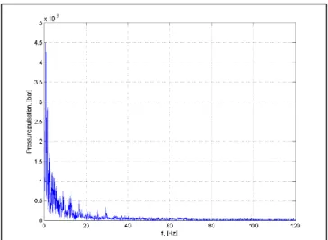
Fig. 18. Δp pulsation spectrum: I = 200A, Q = 0 L/s.
Fig.19. Δp pulsation spectrum: I = 200A, Q = 27 L/s.
Fig. 20. Δp pulsation spectrum: I = 200A, Q = 45 L/s.
Spectrum of pressure pulsation in case of I = 200A and different flowrate is shown in fig. 18 – 20. Signal of 10s was analyzed to obtain each spectrum. One can observe that by increasing the flowrate, overall amplitude of pulsations grows as well as spectrum of LF pulsations becomes broader. In case of high flowrate fig. 19 - 20 it can be observed that some modes of LF pulsations become more dominant. It seems that these modes are somewhat close to 12.5 and 25 Hz which would indicate sub-harmonic phenomenon (from point of view of input frequency).
Domination of some modes in fig. 20 could be caused not only by some effect directly connected to MHD instability but also by e.g. resonance of pressure wave in finite length system. Therefore it is also plausible that in slightly different setup other modes would be more pronounced. However, the question about observed phenomenon is still open to the discussion and requires attention.
In fig. 21 – 23 magnetic field measurements without liquid Na are performed as function of input current. One can observe signal is mostly linearly proportional to applied current and dispersion is mainly caused by positioning error and non-symmetric loading of phases. Also coils (1-2) inside inductor give roughly the same signal up to 2V in case of 200A input current. However signal in 3rd coils is significantly lower – around 0.4 V at 200A.
In fig. 24 – 26 signals of coils as function of flowrate are shown in case of 200A. In fig. 24. one can observe by the shape of curves that signal in 1st coils are not symmetric and tend to be side sensitive (see positioning of sampler in fig. 16.). Rather strong increase of signal is observed from 0.5 – 0.8 V for flowrate 0 - 45L/s.
In 2nd coils (fig. 12.) generally signal is stronger than in 1st coils but has significant dispersion. Increase of signal with flowrate is smaller, roughly 0.2V.
In 3rd coils (fig. 26) for small flowrate signal is higher than in 1st coils, but since they are outside the inductor, signal is practically flow independent.
As discussed before changes in magnetic field measurements suggests strong influence of flow. E.g. high difference in cases of small flowrates between signals of 1st and 2nd coils suggests that flow is positive in side channels but negative in central part. Also higher velocities exist in side channels even when flowrate is increased.
Although absolute values of measurements are not equal to numerical model a qualitative relationship can be established and behaviour of the results is similar. E.g. the increase of voltage in 1st coil is around 0.3V (fig. 24) and in 2nd coil 0.2V (fig. 25). Ratio of voltage increase between channels-1 and 2 are same as in the numerical calculations (0.12 V and 0.08 V accordingly).
Fig. 21. 1st coils signal : U = U(I).
Fig. 22. 2nd coils signal: U = U(I).
Fig. 23. 3rd coils signal: U = U(I).
Fig. 24. 1st coils signal, I = 200A: U = U(Q).
Fig. 25. 2nd coils signal, I = 200A: U = U(Q).
VI. CONCLUSIONS
The investigation of MHD instability phenomenon of large scale ALIP in context of ASTRID project has successfully started. Not only theoretical, but also new experimental and numerical investigation methods have been proposed and conceptualized to be used in PEMDYN facility.
New numerical approaches must be verified with analytical solutions on a basic case study to be used in more sophisticated models. The test case discussed in chapter III.A. show unexpected deviations (higher stability threshold) from analytical solution. Also model suggests that perturbation with amplitude higher than 50% of mean flow influence the developed electromagnetic force significantly. Therefore smaller perturbation (around 10%) could be acceptable. Nevertheless, in such case growth of these perturbations must be controlled. Results show that low frequency pulsations can be also modelled with this approach.
Still, improvements and detailed analysis on both numerical and theoretical models are necessary to compare perturbation growth rates with different Rms and N values.
Presented numerical model of flat EMIP in TESLA-EMP facility shows qualitative resemblance with experimental results where inhomogeneous distribution of magnetic field is detected using set of 24 point measurements. It suggests strong non-homogeneity of the flow and is approved by the numerical model. Experimentally detected low frequency pulsations were not foreseen by numerical model, although longer calculation time is necessary.
Experimental methods in TESLA-EMP facility will be improved in upcoming experiments by increasing amount of magnetic field measurement points, improving positioning of samplers and introducing controlled velocity perturbation in the inlet of the channel to capture perturbation development in the EMIP.
REFERENCES
1. F. GAUCHE et al. “French SFR R&D Program and Design Activities for SFR Prototype ASTRID,” Asian
Nuclear Prospects 2010, p. 314 – 316. Elsevier Ltd.,
(2011).
2. S. VITRY et al., “Development of large flow ALIP EMP for application in ASTRID sodium cooled fast reactor and future power plant reactors,” 8th PAMIR
International Conference September 5-9, Vol. 2, p.551
- 556, Borgo, Corsica, France, (2011)
3. G. RODRIGUEZ et al. “Development of experimental facility platform in support of the ASTRID program,” Intl. Conf. on FAST REACTOR AND RELATED FUEL CYCLES, Paris, France, (2013).
4. A. GAILITIS et al. “Instability of homogeneous velocity distribution in an induction-type MHD machine,” Magnetohydrodynamics, Vol. 1, pp. 87 – 101, (1975).
5. H. OTA et al. “Development of 160m3/min Large Capacity Sodium-Immersed Self-Cooled Electromagnetic Pump,” Journal of NUCLEAR
SCIENCE and TECHNOLOGY, Vol. 41, No. 4, p.
511–523, (2004).
6. H. ARASEKI et al. “Magnetohydrodynamic instability in annular linear induction pump. Part I. Experiment and numerical analysis,” Nuclear Engineering and
Design, Vol. 227, pp. 29 – 50, (2004).
7. L. GOLDSTEINS et al. “Analytical investigation of MHD instability in annular linear electromagnetic induction pump,” 9th International PAMIR Conference,
Vol. 2, pp. 38 – 42, (2014).
8. I. R. KIRILLOV et al. “Local characteristics of cylindrical induction pump when Rms > 1,”
Magnetohydrodynamics, Vol. 2, pp. 95 – 102, (1987).
9. R. A. VALDMANE et al. “Local characteristics of the flow in the channel of an induction MHD machine at large electromagnetic-interaction parameters,”
Magnetohydrodynamics, Vol. 3, pp. 99 – 104. (1977)
10. I. R. KIRILLOV at al. “Low frequency pressure pulsations in annular linear induction pumps,” PAMIR
International Conference September 5-9, Vol. 2,