Adaptive Model-Predictive Climate Policies in a Multi-Country Setting

HAL Id: halshs-00718659

https://halshs.archives-ouvertes.fr/halshs-00718659

Submitted on 17 Jul 2012

HAL is a multi-disciplinary open access archive for the deposit and dissemination of sci-entific research documents, whether they are pub-lished or not. The documents may come from teaching and research institutions in France or abroad, or from public or private research centers.

L’archive ouverte pluridisciplinaire HAL, est destinée au dépôt et à la diffusion de documents scientifiques de niveau recherche, publiés ou non, émanant des établissements d’enseignement et de recherche français ou étrangers, des laboratoires publics ou privés.

Adaptive Model-Predictive Climate Policies in a

Multi-Country Setting

Thierry Bréchet, Carmen Camacho, Vladimir M. Veliov

To cite this version:

Thierry Bréchet, Carmen Camacho, Vladimir M. Veliov. Adaptive Model-Predictive Climate Policies in a Multi-Country Setting. 2012. �halshs-00718659�

Documents de Travail du

Centre d’Economie de la Sorbonne

Adaptive Model-Predictive Climate Policies

in a Multi-Country Setting

Thierry B

Carmen C

Vladimir M. V

Adaptive Model-Predictive Climate Policies in a Multi-Country

Setting

Thierry Br´echet† Carmen Camacho ‡ Vladimir M. Veliov§

Abstract

The purpose of this paper is to extend the use of integrated assessment models by defining rational policies based on predictive control and adaptive behavior. The paper begins with an review of the main IAMs and their use. Then the concept of Model Predictive Nash Equilibrium (MPNE) is introduced within a general model involving heterogeneous economic agents operating in (and interfering with) a common environment. This concept captures the fact that agents do not have a perfect foresight for several ingredients of the model, including that of the environment. A version of the canonical IAM (DICE) is developed as a benchmark case. The concept of MPNE is then enhanced with adaptive learning about the environmental dynamics and the damages caused by global warming. The approach is illustrated by some numerical experiments in a two-region setting for several scenarios.

1

Introduction

Once upon a time there was a world in which people were refusing to see that their world was changing - let’s say because of global warming. The main wish of these many people was to keep on doing their business-as-usual. For sure, the best strategy in the changing world would be for them to learn as much as possible about the expected changes (all of them) and to adopt the optimal behavior with respect to this large set of knowledge. But implementing this optimal strategy was beyond their force or skill. The question we raise in this article is

⇤_{This research was initially supported by the Belgian Science Policy under the CLIMNEG III Project}

(SD/CP/05A). The third author was partly financed by the Austrian Science Foundation (FWF) under grant No I 476-N13. The paper was finalized while Th. Br´echet was visiting research fellow at the Grantham Insti-tute for Climate Change at Imperial College London, and visiting professor at the European University at St Petersburg, Russia.

†_{CORE and Louvain School of Management, Universit´e catholique de Louvain, Voie du Roman Pays, 34,}

B-1348 Louvain-la-Neuve, Belgium, e-mail: thierry.brechet@uclouvain.be

‡_{CNRS and Universit´e Paris 1 Panth´eon-Sorbonne, e-mail: maria.camacho-perez@univ-paris1.fr.} §_{ORCOS, Institute of Mathematical Methods in Economics, Vienna University of Technology,}

not to define what would be the optimal strategy from the whole society’s standpoint (which is already widely explored in the literature) but to highlight possible alternative trajectories, considering that agents are always rational, but sometimes stubborn, lazy or myopic. Stubborn because they always refuse to change their view. Lazy because they revise their view but only after a while (or after some evidence). Myopic because they are more or less short-sighted about how the world will look like in the future. The objective of this article is to explore the consequences of such behaviors in the context of global warming. In this purpose, we develop an innovative theoretical framework to redefine more realistic trajectories of the economies that are fully rational, in contrast with the usual “business-as-usual” scenario defined in integrated assessment models in the current literature.

Our contribution relies on the integrated assessment modeling of the economy and the climate. Integrated means that feedbacks in both ways are considered: economic activity gen-erates greenhouse gases emissions that cause global warming, and global warming a↵ects the economy with productivity and welfare losses. Integrated assessment models (IAMs) allow to implement a dynamic cost-benefit analysis and to determine the optimal policies. Basically, policies in IAMs consist in choosing the path for productive investment and emission abate-ment that maximize some objective function, like country’s welfare. It is important to stress that welfare, in IAMs, is expressed as consumption net of climate damages. It is indeed green consumption that is maximized.

In order to develop this new framework we use the concepts of model predictive control and adaptive behavior, and we combine them into the IAM framework. Ideas from the model predictive control (see e.g. Gr¨une and Pannek, 2011) are employed due to the uncertainties about the future environment and its impact on the economy that the agents persistently face. Adaptive learning or is involved in order to take into account the improvement (with time and/or experience) in the measurements quality and in the agents’ knowledge about the environmental-economic dynamics.

The article is organized as follows. In Section 2, integrated assessment modeling and how it is used for the climate change analysis is presented with some details. This section gathers a condensed explanation of the very concept of IAM, a benchmark model, and a survey of the many uses of IMAs in the literature. In Section 3 we present the general model describing the dynamics of a multi-agent economic-environmental system that will be used in the paper. The concepts of “model predictive rational behavior” and “adaptive behavior” are presented in Sections 4 and 5. The adaptive behaviors considered in this article will concern the knowledge about climate damages (a better knowledge with evidence for climate change) and the discount factor (a decrease in the discount factor as wealth increases). Some numerical experiments are provided in Section 6 with a two-country setting (the world is roughly divided into OECD and non-OECD countries).

2

Integrated assessment of global warming

The purpose of this first section is threefold: (i) to provide the reader with some elements on the history of applied integrated assessment models (IAMs) and its economic rational, (ii) to sketch a benchmark model, (iii) to survey the wide variety of uses of applied integrated assessment models in the literature. This will allow us to better gauge the importance of each contribution we shall introduce later in the paper.

2.1 What is Integrated Assessment?

Although the IPCC reports (1990, 1995, 2001, 2007) had been repeatedly calling for sharp cuts in greenhouse gases emissions (minus 50 to 80 percent at the world level, immediately), they never attempted to balance the costs and benefits of such policies, as it was initially suggested by Nordhaus in 1984.1Nonetheless, balancing costs and benefit has been a prominent methodological and normative contribution of economics for many years. Why not for climate change? Although cost-benefit raises several methodological and theoretical challenges (and it is far beyond the scope of this paper to tackle them; see Pearce et al. (2006) for a comprehensive analysis of CBA analysis and policy applications) it remains a comprehensive framework to understand what should be done, and what could be achieved.

Starting in the early 90s, some aggregative models were developed to analyze the conse-quences of economic activity on greenhouse gases (GHGs) concentration and how this con-centration may harm the economy (see Rotmans, 1990, Nordhaus, 1992 and 1993a, Gaskins et al., 1993, Manne and Richels, 1992, Yang, 1993). These are the very first integrated as-sessment models (IAMs), so-called because they model the economy and its interplay with climate. Economic activity generates greenhouse gases that cause global warming, and global warming provokes physical damages that have an economic cost. IAMs seek at maximizing intertemporal welfare by taking these two components into account. Indeed, it boils down to a standard cost-benefit analysis, but applied to a worldwide and long-term issue.

Basically, the economic part of IAMs is made of a dynamic general equilibrium model of the economy. A policy-maker is assumed to optimally choose consumption/saving path that maximizes the discounted sum of the utility, taking into account how physical capital evolves with time and taking the adverse impacts of climate change into account. In this purpose, IAMs make use of damage functions that translate temperature increase into economic losses. Besides, the policy maker knows the flow of GHGs emissions due to economic activity, how they convert into concentration in the atmosphere and how this concentration a↵ects the average temperature of earth.

In sum, there exists a closed loop between polluting economic human activities, how these

1_{Twenty-three years later, Nordhaus publishes a new book entitled ”A question of balance”. Is it a new}

a↵ect the climate, and how climate change impacts on the economy. What causes global warming is not the flow of GHGs but their accumulation in the atmosphere at a stock. So IAMs are necessarily intertermporal optimisation models. They endogenously determine not only the flow of GHGs but also emission abatement e↵orts and the path of productive investment.

2.2 A benchmark Integrated Assessment Model

The benchmark IAM is based on the DICE model (Dynamic Integrated Climate-Economy model) built up by Nordhaus (1993a, 1993b). DICE is a stylized cost-benefit analysis framework to optimally decide on the trajectory of GHG emissions and capital accumulation at the world level. The model represents a central-planner problem which maximizes the discounted utility taking into account economic and climatic constraints and their interconnection. The economic constraints are those of the Ramsey model.2 _{Output is given by a Cobb-Douglas production}

function, with the peculiarity that a damage function enters multiplying the formulation: Q(t) = ⌦(⌧ )A(t)K(t) P (t)1 ,

where A is a technology index, K physical capital and P population. is the elasticity of output to capital and ⌦ is the afore mentioned damage function. Damage is a function of average temperature ⌧ , and 1 ⌦ is the percentage of foregone production.

Emissions of GHGs flow from the global economic activity (Q) with an exogenous emission factor intensity ( (t)), but taking into account emission abatement e↵orts, denoted by µ ₂ (0, 1). Actual emissions are thus given by:

E(t) = (1 µ(t)) (t)Q(t),

The concentration of GHGs in the atmosphere (M ) is given by past concentration plus new emissions net of the natural decay rate:

M (t) = E(t) + (1 M)M (t 1),

with the atmospheric retention ratio, and M the rate of GHGs absorbed in deep ocean.

Then, an equation is added to give the temperature increase. Nordhaus considers three di↵erent layers: the atmosphere, the mixed layer of the oceans, and the deep oceans. The main link is the damage function, with makes the retroaction between climate and the economy. The damage function represents the economic losses for a given a temperature increase. It is an increasing convex function of global temperature increase:

D(t) = ↵1(T (t)/3)↵2,

2_{We reproduce here the DICE equations taken from Nordhaus (1992), respecting notation, calibration and}

with ↵1, ↵2 2 R+. The last piece of the model is the abatement cost function. Abatement costs

have been extensively studied. This function is thus deemed as more reliable. A 50% decrease in GHGs intensity would cost 1% of the world output. The total abatement cost function is:

C(t) = 1µ(t) 2Q(t).

where µ(t)_{2 (0, 1) is the abatement rate and} 1, 2 are positive constants. Nordhaus uses the

DICE model to compare Business as Usual (defined as µ(t) = 08t) with di↵erent emission stabilization scenarios and the optimal policy. The optimal policy leads to a 10% reduction of carbon emissions from 2005, inducing a temperature decrease of 0.20_{C by 2100 with respect}

to the Business as Usual scenario.

2.3 On the many uses of applied Integrated Assessment Models

Starting from Nordhaus, IAMs have evolved introducing more realistic economic behaviors or outcomes, trying to escape from the basic comparison between BaU (no climate policy, myopic agent) and the socially optimal solution (perfect foresight), because none of them is realistic. In this section, our objective is not to provide an exhaustive survey of IAMs but to review some examples of interesting extensions such as the inclusion of the regional dimension, models with a better description of the power sector, R&D behaviors, and coalition formation issues. A recent survey of these approaches is provided by Stanton et al. (2009).

A direction along which IAMs were developed was geography, and depending on the paper, geography is understood as space or as the union of economic regions. Let us first mention the Integrated Model to Assess the Greenhouse E↵ect (IMAGE) by Rotmans (1990). In its first version, IMAGE was a model integrating three clusters: the energy system, the terres-trial environment system and the atmosphere-ocean system. The second version of the model included a geographical scale, rare at that time. Geography was a grid of 0.5 by 0.5 degrees, making possible the biophysical modeling of land cover, its history, carbon cycle, nutrients, climate, etc. Still, all macroeconomic drivers were exogenous inputs to the model.

In 1996, Nordhaus and Yang extended the DICE model by producing a regional model, RICE (Regional Integrated Climate-economic Model). In this model, the decision is taken at the national level, and the authors consider di↵erent levels of coordination among nations. They propose three di↵erent scenarios to study how nations could deal with climate change: market policies (i.e. no-control on emission), cooperative policies (countries act as a unique decision maker), and non-cooperative policies (in which countries act in their own interests ignoring the externality create on the other countries). These scenarios were labelled “Business-as Usual”, “Cooperative” and “Nash equilibrium” scenarios, respectively. This terminology will be widely used later on in the literature.

Taking DICE or RICE as benchmarks, many authors searched to refine their modeling by incorporating detailed descriptions of the energy sector, allowing for a plethora of mitigation

policies, etc. Edenhofer et al. (2005) introduce learning by doing in R&D, allowing for invest-ment in R&D in di↵erent sectors. In the long term, improving energy efficiency of existing technologies becomes too costly to be kept as the major mitigation policy. Instead, they find that a backstop technology with the potential of learning by doings the best option to protect climate at a lesser cost. They put forward Carbon Capturing and Sequestration (CCS) tech-niques to reduce the cost of the transition from a fossil-fuel based system to a system based on renewable resources.

Bosetti et al. (2006) build the WITCH model (World Induced Technical Change Hybrid Model). WITCH is a multiregional neoclassical growth model in which technological progress is endogenous that is, the price of new vintage of capital and R&D investment are endogenous. The model is hybrid because the energy sector (a key sector) is modeled in great detail, separating electric and non-electric uses of energy, with seven power generation technologies and allowing the use of multiple fuels. The authors account for seven channels for regional interaction. Let us mention amongst them the first, which is the fact that both R&D and consumption decisions are a↵ected by energy prices worldwide. Other interactions are learning by doing, R&D spillovers, international trade of oil and gas, and emissions trading.

The MARKAL-TIMES family of models aims at better describing the technology op-tions, in particular in the power and industry sectors. They are technico-economic models. The modeler needs to introduce technology characterizations and costs, resource availability, environmental constraints, services demands and macro-economic indicators. In this sense, MARKAL-TIMES is much more detailed than other IAMs. In TIMES, the quantities and prices of the various commodities are in equilibrium, i.e. their prices and quantities in each time period are such that the suppliers produce exactly the quantities demanded by the consumers. This equilibrium has the property that the total surplus (consumers plus producers surpluses) is maximized. There also exists a World multi-regional Markal-Times model (Kanudia et al. 2005). Notice that MARKAL models can be developed at all decision levels from wide regions of the world with several countries, to single countries, regions, counties, cities or even villages. Another kind of model is MERGE (Manne and Richels, 2005). MERGE is a model for estimating the regional and global e↵ects of GHGs reductions. The model is flexible enough to explore alternative views on a wide range of contentious issues, such as costs of abatement, damages from climate change, valuation and discounting. The model covers the domestic and international economy, energy-related emissions of greenhouse gases, non-energy emissions of GHGs, global climate change, and market and non-market damages. Each region’s domestic economy is viewed as a Ramsey-Solow model of optimal long-term economic growth. Price-responsiveness is introduced through a top-down production function where output depends upon the inputs of capital, labor and energy bundle. Separate technologies are defined for each source of electric and nonelectric energy.

authority entitled to implement the optimal policy and, second, emission reduction must be worldwide to be e↵ective against global warming. As a result, a wide international agreement among the countries is required, and such an agreement can only be found on a voluntary basis. This is the issue of coalition formation raised by Eyckmans and Tulkens (2003) with the CWS integrated assessment model: which international agreements are feasible, and how to implement them? In other words, between Nash and the socially optimal solution, what inter-national agreement could be achieved? Br´echet et al. (2011) extend this analysis by comparing the policy implications of the two competing theoretical streams available to date, namely, the cooperative and non-cooperative settings.3

3

The dynamics of a multi-agent economic-environmental

sys-tem

Let the global economy consists of n agents (regions, countries or groups of countries) and let xi(t) denote the economic state of the i-th agent at time t (this may include physical capital,

human capital and other dynamic stock-variables, so that xi is a single or multi-dimensional

vector). Let vi(t) be the policy vector of the i-th agent at time t, which may include investments,

abatement and other components. The economic agents operate in a common environment, the state of which may influence the productivity or the utility of the agents. The state of the environment at time t will be represented by a vector y(t), whose components can be the concentrations of GHG in di↵erent sectors of the environment and the average world temperature. Let the economy of the i-th agent be driven by the equation

˙xi(t) = fi(t, xi(t), vi(t), y(t)),

where vi(·) is the chosen by this agent policy (control) function. (Everywhere in this paper

˙x denotes the derivative with respect to the time.) Then the overall dynamics of the world economy is described by the equation

˙x(t) = f (t, x(t), v(t), y(t)), where x = (x1, . . . , xn), v = (v1, . . . , vm), f = (f1, . . . , fn).

On the other hand, the economic activities have impact on the evolution of the environ-ment, say due to emission of GHGs. Let e(t, x, v, y) represents the instantaneous impact vector resulting from global economic state x, control v and environmental state y at time t.

Because GHGs are fungible (they melt in the upper atmosphere irrespective to the country

3_{See also Br´echet and Eyckmans (2012) for a survey on the use of game theory with IAMs, or Yang (2008)}

of origin), the impact vector is represented by the aggregate emissions e(t, x, v, y) = n X i=1 ei(t, xi, vi, y), (1)

where ei(t, xi, vi, y) is the emission of agent i at time t, determined by her economic state,

control, and the environmental state at this time.

We assume that the dynamics of the environment can be represented by an equation of the form

˙y(t) = h(t, e(t, x(t), v(t), y(t)), y(t)).

Thus, given the control function v(·) chosen by the agents, the overall economic-environment system is described by the equations

˙x(t) = f (t, x(t), y(t), v(t)), x(0) = x0, (2)

˙y(t) = h(t, e(t, x(t), v(t), y(t)), y(t)), y(0) = y0, (3) where x0 and y0 are initial data.

In the numerical analysis in this paper we use one simple version of the IAM as described below.

The benchmark model. We specify xi(t) = ki(t) – the physical capital stock of the

i-th agent, vi(t) = (ui(t), ai(t)) – the investment intensity and the abatement e↵ort, y(t) =

(⌧ (t), m(t)) – the average atmospheric temperature at the earth surface and the concentration of GHG (measured in the CO2 equivalent units in the warming context). Equations (2), (3)

are specified as ˙ki(t) = iki(t) + [1 ui(t) ci(ai(t))] ⇡i(t) 'i(⌧ (t)) (ki(t)) i(li(t))1 i, ki(0) = ki0, (4) ˙⌧ (t) = (m(t)) ⌧ (t) + d(m(t)), ⌧ (0) = ⌧0, (5) ˙ m(t) = µm(t) + n X i=1 ei(t, ki(t), ai(t), ⌧ (t)) + ⌫(t, ⌧ (t)), m(0) = m0, (6) with ei(t, ki, ai, ⌧ ) = (1 ai) ⌘i(t)⇡i(t)'i(⌧ )kiil 1 i i .

Since versions of the above most simple IAM are widely used in the literature (see the literature review in Section 2.3) we only shortly explain the appearing notations.

Physical capital accumulation is described by equation (4). The depreciation rate of the physical capital of agent i is i > 0. The labor supply of agent i is li(t) and the production

function is of Cobb-Douglas type with elasticity of substitution i 2 (0, 1). The productivity

of the i-th agent is ⇡i(t) and 'i(⌧ ) is a correction factor for the productivity depending on the

of agent i. It is assumed that the emission (without any costly abatement) is proportional to the output Yi, namely equals ⌘i(t)Yi(t), where ⌘i(t) takes into account the change of emission

per output due to technological change.

A fraction ui(t) of the output is consumed and another fraction, c(ai), is devoted to CO2

abatement at rate ai, the rest is invested, as seen in equation (4). Abatement at rate aireduces

the emission by a factor ai: ei = (1 ai)⌘iYi and costs a fraction ci(ai) of the total product.

The evolution of the CO2 concentration is described by equation (6), where µ is the natural

absorption rate, ⌫(t, ⌧ ) is the non-industrial emission at temperature ⌧ . Finally, (5) establishes the link between CO2concentration and temperature change. The CO2concentration increases

the atmospheric temperature through d but also may a↵ect the cooling rate . The initial values k0_{, ⌧}0_{, m}0 _{are given.}

The control functions vi = (ui, ai) chosen by the agents should satisfy the constraints

ui(t), ai(t) 0, ui(t) + ai(t) 1. (7)

These inequalities define a constraining set V for (ui, ai), which imply in particular, that no

transformation of existing capital into consumption or abatement is possible.

The particular specifications used in the numerical simulations will be given below. The main trouble with the above model and its extensions is that most of the model components are actually not known with certainty. In fact this applies to all of the involved in the benchmark model exogenous functions.

Since the economic agents have to make their policy decisions, vi(t), in conditions of

un-certainty about the future changes of the data, these decisions have to be made on the basis of predictions. Therefore in the next section we develop the concept of prediction-based rational behavior of an individual agent.

In the following two sections we define the two concepts we shall introduce in the IA frame-work: model predictive Nash equilibrium and adaptive behavior. The methodology presented below is not restricted to a specific model. Therefore the exposition is carried out for the gen-eral model (2), (3), while we refer to the benchmark case (4)–(6) only for clarification, and in Section 6 – for numerical simulations.

4

Model predictive rational behavior

Even if the model (2), (3) provides a reasonable description of the dynamics of the real global economic-environment system, it is not exactly known to the agents due to imperfection of the modeling and due to uncertainties in its parameters. That is, at time s agent j chooses her future control policy based on a model that may di↵er from the “true” one. At any time instant s agent j models her economy in her own way, including the impact of the environment on the economy and her own input to the environment. Moreover, the performance criterion of

each individual agent may depend on the time at which the control decision has to be made. Thus at any time s agent j maximizes an individual objective function representing the total (possibly discounted) utility

Z ₁

s

g_js(t, xj(t), vj(t), y(t)) dt (8)

subject to the controlled dynamics

˙xj(t) = fjs(t, xj(t), vj(t), y(t)), xj(s) = xs – known at time s, t s, (9)

˙y(t) = hs(t, ej(t, xj(t), vj(t), y(t)) + ¯ej(t), y(t)) y(s) = ys – known at time s (10)

and the control constraint (see (7) for the benchmark constraints)

vj(t)2 V. (11)

Here g_js is the function that agent j uses at time s for evaluation of the future (discounted) utility, f_js represents the model that agent j employs at time s for predicting the evolution of her economic state xj(t) (for any given future control policy vj(t) and future environmental

state y(t), t s), hsis the model that all agents use at time s for predicting the evolution of the environmental state y(t), t s (given the future total emission e(t)). From the point of view of agent j the total emission e(t) consists of own emission ej(t, xj(t), vj(t), y(t)) depending on

the own control and economic state and on the environmental state y(t), and of the emission of the rest of the agents, ¯ej(t), which is not a priori known to agent j. The environmental

dynamics hs employed at time s is the same for all agents.4

As it will be argued at the end of this and in the next section, this assumption is not too restrictive, since the agents may use the predictions obtained by the environmental model in diverse ways, varying between total ignorance and complete trust.

The interconnected problems (8)–(11) of the n agents at time s are regarded as defining a di↵erential game in which the players (that is, the agents) implement (an open-loop) Nash equilibrium solution. In the next lines we clarify what is the meaning of the Nash equilibrium solution in the present context.

A specific feature of this context is the information pattern. In solving her optimization problem agent j is not necessarily aware of the models f_is that agents i6= j use at time s (as we will see below these models may change with s due to agent-specific adaptive learning). Instead, it is assumed that agent j solves the problem (8)–(11) if the emission ¯ej(t) of the

rest of the agent is given. Let (xs_j[¯ej](t), vjs[¯ej](t), yjs[¯ej](t))), t s, be a solution of problem

4 _{The assumption that all agents use the same environmental model is made only for the sake of simplicity.}

(8)–(11) for the given function ¯ej(t), t s. 5 The resulting emission of agent j is

es_j[¯ej](t) := ej t, xsj[¯ej](t), vjs[¯ej](t), ysj[¯ej](t) .

In the definition of Nash equilibrium it is enough to assume that (instead of the dynamics f_is of all other agents) the emission functional

¯

ej(·) ! esj[¯ej](·) (12)

of each agent is known to the rest of the agents. That is, each agent gives a correct information about her future emissions, given any scenario for the cumulated future emission of the rest of the agents. (This information would be automatically available if the models f_is on which the agent’s decisions are based were known to all agents.) Then the Nash solution consists of an n-tuple of control policies_{vs

i(t)}, trajectories {xsi(t)} of the economies, and emissions {esj(t)},

t s, such that following equilibrium conditions hold for j = 1, . . . , n and t s: v_js[¯es_j](t) = v_js(t) with ¯es_j(·) :=X

i6=j

es_i(t), (13)

xs_j[¯es_j](t) = xs_j(t), (14)

es_j(t, xs_j(t), v_js(t), ys(t)) = es_j(t), (15) where ys is the solution of the equation

˙y(t) = hs(t, es(t), y(t)), y(s) = ys, with es(t) :=

n

X

i=1

es_i(t). (16)

The meaning of the above equalities is the following. Equations (13) and (14) mean that for the cumulated emission ¯es_j(t) of the rest of the agents, agent j will have (xs_j, vs_j) as an optimal solution. Equations (15) mean that the optimal emission of each agent j would equal es

j(t),

provided that the trajectory of the environmental state is ys(·). It remains to notice that due to (15) the equalities

yj[¯esj](t) = ys(t), j = 1, . . . , n

are automatically fulfilled. That is, at the Nash equilibrium solution each agent evaluates the future environmental state in the same way.6

5 _{In this paper we ignore the issues of existence and uniqueness. Some comments on these issues in a slightly}

di↵erent framework are given in Br´echet et al. (2012). In the economic-environmental model in Greiner et al. (2010), for example, the solution does not need to be unique.

6 _{This is the place where the assumption that all agents use the same environmental model h}s _{at any given}

instant s plays a role. If each agent uses its own model hs

j for the environment, then the definition of the Nash

equilibrium solution becomes more complicated and depends on the information pattern: do the rest of the agents know what is the environmental model used by the agent j, or they know only the emission mapping (12). In the later case only a slight modification of the above definition of Nash equilibrium is needed. In the former case the definition of a Nash solution is more complicated.

The numerical calculation consists of iterating the fixed point system (13)–(16). Between 3 and 7 iterations give enough accuracy in the numerical investigation in Section 6.

Now we continue with the definition of the model predictive rational behavior of the economic agents. Let us fix a time-step ✏ > 0 and set sk:= i✏, k = 0, 1, . . ..

At time s = s0 = 0 the agents determine the Nash equilibrium controls{v_is0(t)} resulting

from the models fs0

j , gsj0, hs0 that the agents use at time s0, and from the measurements xsj0,

ys0 _{of the states. The so obtained controls are implemented, however, only in the time-interval}

[s0, s1]. Then the agents update their models and measure the actual state xsj1, ys1. The agents

determine the Nash equilibrium controls_{vs1

i (t)} resulting from the updated models fjs1, gjs1,

hs1 _{and implement them in the time interval [s}

1, s2]. The same procedure repeats further on.

The resulting control policies are ˆ

v_j✏(t) := vsk

j (t) for t2 [sk, sk+1], k = 0, 1 . . . .

The time-step ✏ can be viewed as the length of the commitment periods defined under a legally binding international agreement, like the Kyoto protocol. However, both for mathematical convenience and due to the continual and non-synchronized adjustment of the policies of the agents at micro level, we eliminate the dependence of the control policies on the choice of ✏ letting it tend to zero.

Definition 1. Every limit point of any sequence ˆv✏

j defined as above in the space Lloc1 (0,1)

when ✏ ! 0 (if such exists) will be called Model Predictive Nash Equilibrium (MPNE) policy.7

In practice the time-step at which the actual state of the environment is updated may be many years long due to the slow change of the environment and the relatively high fluctua-tions from the trend. However, the model updates may take place more frequently due to the relatively faster change of the economic states and the progress in the modeling methodologies. We outline the particular case in which an agent j chooses her model fs

j, gjsindependent of the

environmental state y. That is, in her current control policy agent j does not take into account the influence of the future changes in the environmental state on her economy. Accordingly, such an agent disregards the impact of her economic activities on the environment, hence the environmental component (10) is irrelevant for her decisions. In Br´echet et al. (2012) we interpret such an agent as doing Business as Usual (BaU). A BaU agent disregards her interconnections with the environment and, consequently does not abate emissions. We stress that the above notion of BaU di↵ers from the one used in the literature (see e.g. Nordhaus and Yang, 1996), where BaU is an agent who does not abate, although having a foresight about the influence of the future environmental changes on the economy.

7_{A sequence v}✏_{converges to v in L}loc

1 (0,1) if

RT

0 |v

✏_{(t) v(t)}

In the above consideration the models of the individual economic dynamics and objectives of the agents, as well as the model of the environment, are considered as given, although changing with the time in a non-anticipative way (the future changes in the models are not known, hence not involved in the formation of the current control policies). In the next section we partly endogenize the evolution of the models that agents employ by using a simple version of adaptive learning.

5

Adaptive behavior

At any time s the agents use models (given by the triplet (fs

j, gsj, hs)) to determine their policy

for some period of time after s, as described in the previous subsection.

In this subsection we address the following question: how the agents change the models that they use, depending on the newly available measurements of the actual economic and environmental states?

A variety of data assimilation techniques can employed for this purpose, out of which a simple adaptive learning is chosen in this paper.

For the sake of clarity and for numerical simulations we consider here only the benchmark model. The environment is assumed to be relevantly described by equations (5), (6), thus in this case hs= h for all s. Moreover, we apply adaptive learning to only two crucial uncertain factors that may vary with the time at which the control decisions are taken and that essentially influence the behavior of the agents: the damage function which represents the e↵ect of the climate change on the economy, and the discount rate used by the agents in the formulation of their future objectives. It is reasonable to apply adaptive learning to many other economic factors, such as future productivity, ⇡i(t), future labour li(t), future emission per output, ⌘j(t),

future natural emission, ⌫(t), etc., but here we assume a perfect knowledge for their evolution. In the benchmark case the model (9)–(11) that agent j uses at time s reads as

˙kj = jkj+ [1 uj cj(aj)] ⇡j'sj(⌧ ) kjjl 1 j i , kj(s) = kjs, (17) ˙⌧ = (m) ⌧ + d(m), ⌧ (s) = ⌧s, (18) ˙ m = µ m + (1 aj) ⌘j⇡j'sj(⌧ ) kjjl 1 j i + ¯ej+ ⌫(⌧ ), m(s) = ms, (19) uj(t), aj(t) 0, uj(t) + aj(t) 1. (20)

To complete the benchmark agent’s model we consider a particular objective function gs j in (8) defined as Z ₁ s e rjst ⇥_{uj(t) ⇡j(t) '}s j(⌧ (t)) (kj(t)) j(lj(t))1 j⇤1 ↵ dt, (21) where rs

As already said, the model components that the agent j updates at time s (based on the available measurements for kj(t) and ⌧ (t) till time s) are the damage function 'sj(⌧ ) the

discount rate rs_j.

5.1 Updating the damage function

In the next paragraphs we analyze how agents with diverse level of knowledge and concerns or with diverse opinion about the reliability of the presently used environmental models and monitoring (in our case (18), (19)) may build their formal estimates about the influence of the global warming on their regional economic efficiency.

Below it will be assumed that the true damage on the productivity in the region of agent j caused by a temperature increase ⌧ above the pre-industrial level is given by the formula

'(⌧ ) = 1

1 + ✓_⇤⌧, (22)

where  is a known constant and the value of ✓_⇤ is not known to the agent (considering also  or more parameters as unknown does not bring principal di↵erence). The above constants are agent-specific, but we skip the index j in the notations since the considerations below apply to an individual agent.

As a specification of the benchmark model we assume that at any time s instead of the “true” damage function (22) for her region agent j uses the following one:

's(⌧ ) = 1

1 + ✓s( s⌧s+ (1 s)⌧ )

, (23)

where ✓s represents the current estimate of the true value ✓⇤, ⌧s is the measured average

temperature at time s, and s 2 [0, 1] is an additional parameter chosen by the agent at

the current time s. As argued below, this parameter reflects the level of confidence in the environmental model (18), (19). Notice that at the current time s the temperature is ⌧ (s) = ⌧s, hence the evaluation of the damage function gives

's(⌧ (s)) = 1 1 + ✓s⌧ (s)

. (24)

Since the true value of the damage is measurable, the agent may calculate the value ˜✓sthat fits

to the current measurements of ⌧ (s) and '(⌧ (s)). Due to the uncertainties in the measurements the agent evaluates the parameter ✓s to be used in her current model as

✓s= ✓s + "⇢s(˜✓s ✓s ),

where ✓s is the agent’s estimation of ✓ prior to time s (which depends on past measurements).

The parameter ⇢s2 [0, 1] reflects the agent’s uncertainty about the currently estimated factors:

temperature, capital stock, economic output: the lower is the confidence of the agent, the smaller is ⇢s. The parameter " > 0 is the time step for updating the damage function, as in the

preceding subsection. In the limit case with "_{! 0 and ⇢}s = ⇢ the value ⇢ can be interpreted

as the exponential decay rate of the error: ✓_⇤ ✓s= e ⇢s(✓⇤ ✓0).

On the other hand, at time s the agent employs the damage function in her long-run investment/abatement planning model (17)–(21), as described in the previous subsection. Since the temperature ⌧ may change in the future and the agent uses the environmental model (18), (19) to predict this change, the anticipated error in ⌧ produced by the model may distort the predicted damage rate. To take into account these uncertainties the agent modifies the damage function (24) in the way given by (23). The argument for choosing a damage function in the form of (23) is shortly explained below, taking for simplicity the value  = 2.

At time s the agent has updated her damage function 's by choosing the new parameter ✓s in (24) as described above. However, the agent realizes that the true temperature at time

t > s may be di↵erent from the one resulting from the model (18), (19), with an error ⇠ = ⇠(t). Then the anticipated value of the damage function, when using (23) at time t and with the true temperature ⌧ = ⌧ (t) will be

1

1 + ✓s( ⌧s+ (1 )(⌧ + ⇠)2)

.

Since ⇠ can be viewed as a random variable (although its distribution is unknown), the rational agent would try to minimize by choosing the parameter _{2 [0, 1] the expectation}

E ✓ 1 1 + ✓s⌧2 1 1 + ✓s( ⌧s+ (1 )(⌧ + ⇠)2) ◆2! .

Having in mind that ✓_⇤, hence also ✓, is a small number (✓_⇤ = 0.0054 according to Nordhaus, 2007), one can reasonably represent the above expression as

✓2_sE⇣ ( + 2⌧ ) + 2( + ⌧ )(1 )⇠ + (1 )2⇠2 2⌘+ O(✓_s3), (25) where = ⌧s ⌧ and O(")/" is bounded when "! 0. From here one can make the following essential observation:

(i) if the agent trusts the employed environmental model (hence ⇠ = 0), then this agent would choose = 0, which gives value zero in the error-expectation formula (25);

(ii) if the agent does not believe in the long run trend of the temperature change (assuming = 0) and anticipates an error ⇠6= 0 of the model-base prediction for the temperature, then this agent would choose = 1.

The analysis may be continued by considering the optimal choice of the parameter , that is, choosing the that minimizes the expression in (25). We skip this technical (and not very precise) consideration, which suggests that an agent whose opinion about the accuracy of the environmental model (18), (19) measured byP4_n=1|E(⇠n_{)| is large relative to the expected by}

the agent temperature change = ⌧ ⌧s _{(a “skeptical” agent), then this agent would choose}

would choose closer to zero. Of course, the same learning procedure as for ✓ can be applied also for .

Summarizing, one may say that the choice of the predictor for the future damage caused by the global warming is a subjective decision of the agent, which can be formally characterized by the following statement in terms of the parameters ⇢s and s in the update of the damage

function: agents who are sceptic about the measurements (and the model) of the economy and about the measurement of the current temperature choose lower value of ⇢s; agents who are

sceptic about the credibility of the employed environmental model choose a higher value for the parameter s 2 [0, 1].

We note that an agent choosing = 1 makes no use of the environmental model at all, since this agent always takes the current temperature as a proxy for the future one. Thus = 1 represents a BaU-agent. In the present framework the agents are distinguished by their parameters ⇢s and sand the BaU agent is an extreme case in a continuous variety of agents.

5.2 Updating the discount rate

The discount rate r_js chosen by agent j at time s in its utility function represents her opinion about the value of the present utility relative to a future one. Of course, the discount rate rs j

depends on the agent’s view on the future uncertainty, but in the context of the environmental concerns it depends also on the agent’s per capita wealth. As one can clearly see from the daily practice, a rich country tends to be more far-sighted than a poor country in which the political and the economic policies are more myopic. Similar suggestions are given in the economic literature (see e.g. Lawrence, 1991, and Samwick, 1998). Therefore, it is reasonable to assume that the discount rate of agent j depends on her per capita wealth measured at time s by kj(s)/lj(s) = kjs/lj(s) (where labor is proportional to the population size). Thus,

at time s the agent would have an endogenous discount rate rs_j = R(k_js/lj(s)). The particular

specification of the function R used in the subsequent numerical analyses is given in Section 6.

6

Some simulation results

The agents in the benchmark model (17)–(21) are heterogeneous with respect to all involved parameters. However, we shall focus on the heterogeneity with respect to their behavioral features, represented by the damage function 's_j(⌧ ) and the discount rate r_jsused at time s by agent j.8

8_{The adjective “behavioral” indicates dependence on subjective attitude of the agent. Moreover, the agents}

6.1 Model calibration

The individual damage function used by an agent at time s is characterized in the previous section by three parameters: the knowledge about the “true” damage function prior to s, denoted by ✓s , the learning parameter ⇢s, and the “trust” parameter s. Diverse values

of these parameters and of the discount rate rs

j allow to cover agents with rather di↵erent

behavior, including such doing BaU (see the end of Section 4), myopic versus far-sighted agents, sceptical about the accuracy of the climate predictions versus “believers”, etc. Given any configuration of agents, their (interconnected) economic behaviour is defined in Section 4 by the Model Predictive Nash Equilibrium (MPNE).

Although the concept of MPNE applies to any number of agents, in the simulation results below we consider for more transparency only two agents. The first agent, named agent R (from “Rich”), is presumably richer, hence less discounting the future, has better knowledge on the damage function and trusts more the predictions for the climate change. The second one, agent P (from “Poor”), is presumably poorer, hence more myopic, has bad knowledge on the damage function but may learn with experience, and is skeptical about the predictions for the climate change. In the benchmark model agents R and P are indexed by i = 1 and i = 2, respectively.

The prototypes of these two agents in some of the simulations below are the OECD and the non-OECD countries, respectively. Therefore in all simulations 74.7% of the world physical capital stock (estimated as 733.2 trillion USD in 2005) belongs to agent R, while the rest of 25.3% belongs to agent P. Thus the initial data for the economy are k₁0 = 547.7004 and k0

2 = 185.4996 trillion USD. On the other hand, the population of agent R is 18.2% of the total,

which gives l1 = 0.184L, l2 = 0.816L with the total population L = 6464.75 million. The initial

data for the environment are m0 _{= 808.9 and ⌧}0 _{= 0.7307, representing the concentration of}

CO2in GtC and the increase of temperature above the pre-industrial level in 2005, respectively.

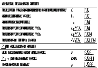
The constant parameters of the benchmark model are given on Table 1. The calibration year is 2005.

The functional parameters in the benchmark model are specified as follows.

Due to technological progress the productivity ⇡i(t) is assumed linearly increasing with

time so that technology is 25% more efficient after 175 years, that is, ⇡i(175) = 1.25⇡i(0) for

i = R, P .

The technological progress reduces the emission per unit of output (without abatement) at an exponential rate 0.00384, which corresponds to a decrease by 25% in 75 years: ⌘i(t) =

e 0.00384t_⌘

i(0). The cost-of-abatement function ci(a) = c(a) is specified as c(a) = 0.01a/(1 a),

which implies that reducing emission by 50% incurs cost of 1% of GDP. The true damage function for all agents is assumed to be

'⇤(⌧ ) = 1

Table 1:Values of stationary parameters

Economic parameters

intertemporal elasticity of substitution ↵ 0.5

depreciation rate i 0.1

capital elasticity i 0.75 initial productivity of R ⇡1(0) 1.75 initial productivity of P ⇡2(0) 1.17 initial emission rate ⌘i(0) 0.0427 Climate parameters

temperature stability rate 0.11 CO2 absorption rate µ 0.0054

natural emission ⌫ 3.211

(of course it is not assumed to be known to the agents).

Finally, the e↵ect of CO2 concentration on the average temperature increase is captured

by the standard function d(m) = 0.5915 ln(m/m⇤₀), where m⇤₀ = 596.4 GtC is the preindus-trial CO2 concentration in the atmosphere. All the specifications are within usually suggested

ranges.9

6.2 Scenarios description

For the behavioral parameters 's

j(·) in (23) and the discount rate rsj we consider several

scenarios as described below.

Scenarios 1 and 2. These are two “extreme” scenarios. In Scenario 1 both agents are myopic and totally neglect the environmental dynamics in their decisions, adapting to the temperature change only post factum (this is what we called BaU agent in the end of Section 4). Precisely, agent R has the parameters rs₁= r1= 0.02 (myopic), ✓s= ✓⇤ (evaluates correctly her damage

at the current temperature ⌧s_{), = 1 (ignores the prediction for future change of temperature),}

⇢ is irrelevant. Agent P has the same parameters with the only di↵erence that ✓s = ✓⇤/6 and

⇢ = 0 (underestimates the damage of the current temperature and does not learn).

In Scenario 2 we consider that both agents as far-sighted, perfectly informed about the environmental dynamics and the damage function. Precisely, for both agents rs_i = 0.005, ✓s= ✓⇤, s = 0. In fact, in this case the MPNE coincides with the usual Nash equilibrium due

to the perfect foresight of both agents.

Scenario 3. In the third scenario we take into account that agent P may learn and may become less sceptic with experience, still remaining myopic. The role of this scenario is to

exhibit the e↵ect of learning. Formally, agent R is exactly as in Scenario 2, while agent P has rs

2 = 0.02, ✓s = ✓⇤ e ⇢s(✓⇤ ✓0), with ✓0 = ✓⇤/6, ⇢ = 0.03465, and s = e ⇢s. The chosen

value of ⇢ means that agent P reduces the error in ✓ by half and the value of the distrust parameter from 1 to 0.5 in 20 years.

Scenario 4. This last scenario involves endogenous discount for agent P, all the rest is as Sce-nario 3. Agent P is initially myopic (r0₂ = 0.02), but her discount rate decreases quadratically with the per capita stock of capital till the value r = 0.005 is achieved when the capital stock reaches the initial value of the initial capital stock of agent R. That is, at this point agent P starts discounting as low as agent R, who has r1 = 0.005 all the time.

In all scenarios the agents use the investment and the abatement rates, ui(t) and ai(t), as policy

instruments. Of course, in Scenario 1 the agents have no reasons to abate (hence aj(t) = 0).

6.3 Simulation results

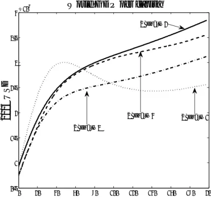
The four scenarios are graphically depicted in figures1-3. Our results support the intuitive idea that the more you know the better you do. Indeed, Scenario 2 represents the economy with the best informed individuals who care the most about the future. On the other side, agents in Scenario 1 are myopic about global warming and do not care much about the future. On top of this, they are unable to learn. This implies that they never revise their vision about global warming nor do they increase their concern about the future. They are stubborn and short-sighted, which are rather common psychological features in the the real word. As a result, in short, Scenario 2 provides the highest consumption and GDP per capita in the long-term, incurring in the lowest increase in temperature while Scenario 1 provides the worst results.

A striking result to be mentioned about these two scenarios is the shape of GDP (or consumption) over time. After an increase in GDP per capita at the beginning of the simulation period, Scenario 1 displays a shrink in the level of the world GDP by 25% in 90 years. This reflects the economic consequences of neglecting climate change. Actually, in Scenario 1 World GDP declines by 0.3% per year between time 50 and 140. In the same period of time world GDP increases by 0.3% per year on average in Scenario 2. This shows how a more realistic definition of a BaU translates into climate costs on the economy. Let us remind that we use the same calibration parameter values as Nordhaus (2007). What makes the di↵erence is the rational behind the scenarios. Clearly, this result sheds a new light on the potential costs of no-action against global warming. Most people agree that emission abatement is costly but forget that climate change itself is costly to the economy. This simulation reveals that these costs may be much higher than usually appraised with IAMs because of they ill-define what is business-as-usual.

After 100 years, Scenario 2 induces a temperature increase of less than 3 C, providing a GDP of 30,000 USD per capita. Scenario 1 provides higher consumption during the first 90

0 20 40 60 80 100 120 140 160 180 200 0.5 1 1.5 2 2.5 3 3.5 4x 10

4

World GDP per capita

2005

US

D

Figure 1: World GDP per capita.

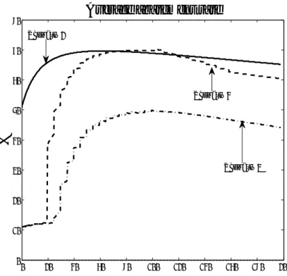
years, given that agents do not abate. Nevertheless, because they incur in the largest emissions, their productivity is harmed the most. In order to preserve a high level of consumption during the entire period, agents in Scenario 2 abate more than 50% of their emissions, attaining up to 70% after 50 years. Given that agents do not abate at all in Scenario 1, temperature increases by more than 6.5 C after 100 years, which dampens their productivity and hence their income. Naturally, Scenarios 3 and 4 provide results that lie in between Scenario 1 and 2, getting closer to Scenario 2 as the amount of information and concern about the future increase. Scenarios 3 and 4 are similar during the first 20 years. Di↵erences arise after and one can observe the behavioral di↵erences between agents who update their discount rate, and those who do not. In Scenario 3, agent R knows exactly the damages induced by global warming, and she discounts future at at a higher rate. On the other side, agent P, who does not abate at the beginning, starts soon doing so, adding her e↵ort to agent R’s. However, agent P’s lack of care about the future impedes larger abatement e↵orts. Consequently, GDP per capita and consumption are larger than in Scenario 1, and temperature increase after 100 years is 3.75 C above the preindustrial level. Therefore, although this economy starts abating a 10% of their emissions on the average, it gradually increases abatement e↵orts until 50% after one century. Finally, building on Scenario 3, we allow agent P in Scenario 4 to become more patient as she becomes wealthier. Hence, as agent P accumulates wealth with time, she starts caring more about its future and increases her abatement e↵ort accordingly. We can see in figure 2 that the average abatement rate equalizes Scenario 2’s after 70 years and then over-reach it

0 20 40 60 80 100 120 140 160 180 200 0 10 20 30 40 50 60 70

80

Average abatement rate

%

Scenario 3 Scenario 4 Scenario 2

Figure 2: Average abatement rate.

for some decades. Agents get very close to Scenario 2 in terms of consumption and GDP as well, but they cannot catch them because of the damages accumulated on productivity during the first 60 years.

It is interesting to notice that, although Scenario 2, 3 and 4 are relatively close in terms of temperature increase, they display contrasting profiles regarding GDP, consumption, and abatement policies. For example, in Scenario 4 abatement e↵orts are stronger than in the “optimistic” Scenario 2 for most time periods because of the delay incurred by the endogenous discounting. It shows that the idea of relying on endogenous discounting (driven by economic development) to cope with global warming is inadequate because it takes too long.

It is interesting to compare the aggregated discounted utility of agent R (given by (21) on a 200 years long horizon) in scenarios 2 and 4. The discount factor of agent R is r = 0.005 in each of these scenarios, therefore the results are comparable: the values are 52,995 in Scenario 2 and 37,022 in Scenario 4. Since agent R has exactly the same parameters in the two scenarios, the reason for the large di↵erence of her welfare is caused by agent P. Notice that due to learning and due to the endogenous discount, after 100 years agent P in Scenario 4 behaves exactly as agent P in Scenario 2: has a perfect knowledge and discounts with r = 0.005. However, due to the delay in the evolution of agent P from a myopic ignorant to a far-sighted knowledgeable agent (as R is from the very beginning), agent R loses about 30% of her 200-years utility. This result shows how important it is for the rich country to help the poor one to develop, because both share the same common good, climate.

0 20 40 60 80 100 120 140 160 180 200 0 1 2 3 4 5 6 7 8

Temperature increase

C

Figure 3: Temperature increase.

7

Conclusion

The purpose of this article was to extend the standard integrated assessment framework applied to climate change by incorporating model predictive control and adaptive behavior. Model predictive control is employed due to the uncertainties about the future environment. It allows agents to redefine their optimal strategy on a regular basis, on the grounds of the observed changes in the world or in the agents’ time preferences (endogenous discounting in our model). With this setting, agents are rational (they adopt the optimal policy) but revise it (with some inertia) as the word changes. Adaptive behavior (or learning) is involved since the agents gradually improve their knowledge about the world (the interconnection between environment and economy, in our model). These ingredients are particularly relevant in the context of global warming. We provide a generic theoretical model encompassing all elements of an integrated assessment model. In particular, we define an innovative concept of Model Productive Nash Equilibrium (MPNE) to characterize an economy with many countries. Simulations show, among other results, how the trajectory of the economy can be a↵ected by the adaptive configuration. In particular, a pessimistic configuration (pessimistic, but maybe not so far from reality) displays a shrink in the world GDP due to the adverse e↵ects of climate change and the persistent agent’s will to disregard them. This new framework would deserve to be extended in several directions. A first natural one would be to split the word in many countries or regions. In this case, strategic interactions among countries would become a new ingredient of the framework.

References

Bosetti V., C. Carraro, M. Galeotti, E. Massetti, M. Tavoni (2006). “WITCH: A World Induced Technical Change Hybrid Model”, The Energy Journal, Special Issue 2, 13-38.

Br´echet T., Camacho C. and Veliov V. (2011). “Model predictive control, the economy, and the issue of global warming”, Annals of Operations Research, DOI 10.1007/s10479-011-0881-8. Br´echet T., G´erard F. and Tulkens H. (2011). “Efficiency vs. stability of climate coalitions: a conceptual and computational appraisal” The Energy Journal 32(1), pp. 49-76.

Br´echet T. and Eyckmans J. (2012). “Coalition Theory and Integrated Assessment Mod-eling: Lessons for Climate Governance”, in E. Brousseau, P.A. Jouvet and T. Dedeurwareder (eds). Governing Global Environmental Commons: Institutions, Markets, Social Preferences and Political Games, Oxford University Press, forthcoming, 2012.

Edenhofer O., N. Bauer, E. Kriegler (2005). “The impact of technological change on climate protection and welfare: Insights from the model MIND”, Ecological Economics, 54, 277-292.

Eyckmans J. and Tulkens H. (2003). “Simulating coalitionally stable burden sharing agree-ments for the climate change problem”, Resource and Energy Economics, 25, pp. 299-327.

Gaskins, D.W. Jr. and J. P. Weyant (1993). “Model Comparisons of the Costs of Reducing CO2 Emissions”, The American Economic Review, Vol. 83, No. 2, 318-323.

Greiner, A., L. Gruene and W. Semmler (2010). “Growth and climate change: threshold and multiple equilibria”, in J. Crespo Cuaresma, T.P. Palokangas and A. Tarasyev (eds), Dynamic Systems, Economic Growth, and the Environment, Springer-Verlag, pp. 63-79.

Gr¨une, L. and J. Pannek (2011). Nonlinear model predictive control, Springer, London. Kanudia A., Labriet M., Loulou R., Vaillancourt K. and Waaub J-Ph. (2005). “The World-Markal Model and Its Application to Cost-E↵ectiveness, Permit Sharing, and Cost-Benefit Analyses ” Energy and Environment, pp. 111-148.

Keller E., M. Spence and R. Zeckhauser (1971). “The Optimal Control of Pollution”, Journal of Economic Theory, 4, 19-34.

Lawrence, E. C. (1991). “Poverty and the rate of time preference: evidence from panel data”, Journal of Political Economy, 99, 54-75.

Manne, A.S., R. Richels (1996). “Buying greenhouse insurance: The economic costs of CO2

emission limits, MIT Press.

Manne, A.S., R. Richels (2005). “Merge: An Integrated Assessment Model for Global Cli-mate Change”, Energy and Environment pp. 175 - 189.

Nordhaus W. (1977). “Economic Growth and Climate: The Case of Carbon Dioxide”, The American Economic Review, Vol. 67, No. 1, pp. 341-346.

Nordhaus, W.D. (1992). “An Optimal Transition Path for Controlling Greenhouse Gases”, Science, 258, 1315-1319.

Ap-proach” with T. A. Daly, N. Goto, and R. F. Kosobud, in John Weyant, ed., The Energy Industries in Transition, Part I, International Association of Energy Economists, Washington, D.C., pp. 547-561.

Nordhaus, W.D. and Z. Yang (1996). “A Regional Dynamic General-Equilibrium Model of Alternative Climate-Change Strategies”, The American Economic Review, Vol. 86, No. 4, pp. 741-765

Nordhaus W. (1993a). “Rolling the DICE: An Optimal Transition Path for Controlling Greenhouse Gases”, Resource and Energy Economics, 15, pp. 27-50

Nordhaus W. (1993b). “Optimal Greenhouse-Gas Reductions and Tax Policy in the DICE Model”, American Economic Review, Vol. 83, No. 2, pp. 313-317.

Nordhaus W. (2007). “A Review of the Stern Review on the Economics of Climate Change,” Journal of Economic Literature, American Economic Association, vol. 45(3), pp. 686-702.

Pearce D., Atkinson G., Mourato S. (2006). Cost-Benefit Analysis and the Environment: Recent Developments OECD, Paris.

Rotmans, J. (1990). IMAGE: an integrated model to assess the greenhouse e↵ect, Springer. Samwick, A. (1998). ” Discount rate homogeneity and social security re- form”, Journal of Development Economics, 57, 117-146.

Stanton E.A, Ackerman F. and Kartha S. (2009). “Inside the integrated assessment models: Four issues in climate economics”, Climate and Development, 1(2), pp. 166-184.

Stern N. (2006). The Economics of Climate Change: The Stern Review, Cambridge, UK: Cambridge University Press.

Yang Z. (1993). “Essays on the International Aspects of Resource and Environmental Economics”, Ph.D. dissertation, Yale University.

Yang Z. (2008). Strategic Bargaining and Cooperation in Greenhouse Gas Mitigations - An Integrated assessment Modeling Approach, MIT Press.