Life tables and Leslie matrices for mammalian cohorts in different paleobiological contexts during the Pleistocene

(1)

HAL Id: hal-02467896

https://hal.archives-ouvertes.fr/hal-02467896

Submitted on 20 Nov 2020

HAL is a multi-disciplinary open access

archive for the deposit and dissemination of

sci-entific research documents, whether they are

pub-lished or not. The documents may come from

teaching and research institutions in France or

abroad, or from public or private research centers.

L’archive ouverte pluridisciplinaire HAL, est

destinée au dépôt et à la diffusion de documents

scientifiques de niveau recherche, publiés ou non,

émanant des établissements d’enseignement et de

recherche français ou étrangers, des laboratoires

publics ou privés.

Life tables and Leslie matrices for mammalian cohorts in

different paleobiological contexts during the Pleistocene

Philippe Fernandez, Christophe Bonenfant, Jean-Michel Gaillard, Serge

Legendre, Hervé Monchot

To cite this version:

Philippe Fernandez, Christophe Bonenfant, Jean-Michel Gaillard, Serge Legendre, Hervé Monchot.

Life tables and Leslie matrices for mammalian cohorts in different paleobiological contexts during the

Pleistocene. Jean-Philip Brugal (dir.). TaphonomieS, Editions des Archives contemporaines,

pp.477-497, 2017, TaphonomieS, 9782813002419. �hal-02467896�

(2)

9HSMILD*aacebj+

Prix public : 67 euros ISBN : 9782813002419

TaphonomieS

Des ossements d’éléphant dans une grotte ; de bison dans un dépôt lacustre ; des restes humains et des outils lithiques associés à des fossiles de lions ou d’hyènes… Éléphant cavernicole, bison aquatique, chasseurs ou chassés ? Ces exemples préhistoriques nous interpellent quant à leurs origines et aux associations qu’ils suscitent.

Comment ces accumulations du passé touchant un vaste éventail d’objets (faune, flore, productions humaines…) se sont-elles constituées et conservées au cours du temps, durant des centaines, des milliers, ou des millions d’années ? C’est dans cette perspective que se placent les études en taphonomie, largement pluri- et inter-disciplinaires, intégrant de multiples approches scientifiques. L’ouvrage décline ces approches dans le cadre temporel du Quaternaire (les trois derniers millions d’années environ), contemporain de l’apparition et de l’évolution de la lignée humaine et des grandes glaciations de l’hémisphère nord de la planète.

Depuis la molécule et la cellule jusqu’aux organismes, parcellaires ou complets, la taphonomie – ou plutôt les « TaphonomieS » –, science plurielle, forme un nouveau champ d’analyses particulièrement fécond et fédérateur. Ce livre a pour objectif à la fois d’en révéler la démarche et de présenter un certain nombre d’études conduites par des équipes françaises. Du passé au présent, et vice-versa, cette « nouvelle » discipline devrait et doit intéresser non seulement tous les chercheurs et étudiants travaillant sur des vestiges du passé selon des reconstitutions systémiques, mais aussi les acteurs actuels de nos sociétés « anthropocènes », productrices de nombreux déchets et vestiges qui nous survivront, on ne sait dans quelles conditions et états… ?

L’ouvrage concrétise les travaux du groupement de recherches « Taphonomie, En-vironnement et Archéologie » (TaphEnA) du CNRS-INEE. Divisé en six parties, il regroupe vingt-sept chapitres rédigés par quarante-cinq auteurs de diverses spécialités des sciences de la Terre, de la vie, et des sciences humaines.

Avec les contributions de William E. Banks, Cedric Beauval, Pascal Bertran, Olivier Bignon-Lau, Christophe Bonnenfant, Jean-Guillaume Bordes, Laurent Bouby, Nicolas Boulbes, Jean-Philip Brugal, Dominique Castex, Julia Chrzavzez, Dries Cnuts, David Cochard, Patrice Courtaud, Jean-Pierre Cuif, Camille Daujeard, Yannicke Dauphin, Claire Delhon, Alain Denis, Christiane Denys, Henri Duday, Philippe Fernandez, Jean-Baptiste Fourvel, Jean-Michel Gaillard, Jean-Bernard Huchet, Sacha Kacki, Vincent Lebreton, Pierre Magniez, Bruno Maureille, Pierre Massard, Anne Marie Moigne, Hervé Monchot, Paul Palmqvist, M. Patrocinio Espigares, Alain Person, William Rendu, Veerle Rots, Marie-Pierre Ruas, Géraldine Sachau-Carcel, Loïc Ségalen, Isabelle Thery-Parisot, Vera Tiesler, Dominique Todisco, Aurore Val et Luc Vallin.

TaphonomieS

Coordinat ion

GDR 3591

CNRS-INEE

et

Je

an-Philip Br

ug

Groupement de recherches 3591

« Taphonomie, Environnement et Archéologie »,

CNRS-INEE

Sous la direction de

Jean-Philip Brugal

TaphonomieS

Colle

ct

ion

Sc

ie

nc

es

arc

hé

ologique

s

Collection

Sc

iences

arc

héologiques

Ouvrage du

Groupement de recherches 3591

« Taphonomie, Environnement et Archéologie », CNRS-INEE

(3)

(4)

(5)

TaphonomieS

Ouvrage du Groupement de recherches « Taphonomie, Environnement et Archéologie », CNRS-INEE

Sous la direction deJean-Philip Brugal

(6)

représentation intégrale ou partielle, par quelque procédé que ce soit (électronique, mécanique, photocopie, enregistrement, quelque système de stockage et de récupération d’information) des pages publiées dans le présent ouvrage faite sans autorisation écrite de l’éditeur, est interdite.

Éditions des archives contemporaines 41, rue Barrault 75013 Paris (France) www.archivescontemporaines.com ISBN 9782813002419 9 782813 002419 Illustration de couverture :

Tissu Kuba en fibres naturelles (appelé aussi shoowa, raphias / velours Kasaï), du Zaïre-Congo (Afrique). © photo J.-Ph. Brugal

Avertissement : Les textes publiés dans ce volume n’engagent que la responsabilité de leurs auteurs. Pour faciliter la lecture, la mise en pages a été harmonisée, mais la spécificité de chacun, dans le système des titres, le choix de transcriptions et des abréviations, l’emploi de majuscules, la présentation des références bibliographiques, etc. a été le plus souvent conservée.

(7)

Collection « Sciences archéologiques »

dirigée par Philippe Dillmann

Sous le parrainage :

o du réseau CAI-RN (Compétences archéométriques interdisciplinaires – Réseau national) de la Mission pour l’interdisciplinarité du CNRS http ://archeometrie.cnrs.fr

o du réseau GMPCA (Groupe des méthodes pluridisciplinaires contribuant à l’archéologie)

https ://gmpca.fr

Membres du comité scientifique :

Marie Balasse, Sandrine Baron, Sylvain Bauvais, Ludovic Bellot-Gurlet, Jean-Philip Brugal, Emmanuelle Delqué-Kolic, Eva-Maria Geigl, Estelle Herrscher, Guillaume Hulin, Philippe Lanos, Matthieu Le Bailly, Matthieu Lebon, Joséphine Lesur, François-Xavier Le Bourdonnec, Anne-Solenn Le Hô, Chantal Leroyer, Vivien Mathé, Norbert Mercier, Valérie Merle, Chris-tine Oberlin, Ina Reiche, MarChris-tine Regert

(8)

(9)

Life tables and Leslie matrices

for mammalian cohorts in different

paleobiological contexts during

the Pleistocene

Philippe Fernandez

1

_{, Christophe Bonenfant}

2

_,

Jean-Michel Gaillard

2

_{, Serge Legendre}

3

_{, Hervé Monchot}

4

1_{UMR 7269 LAMPEA, Aix-en-Provence, Université Aix-Marseille – CNRS – MCC} 2_{UMR 5558, Lyon – UCB Lyon 1 – CNRS} 3_{UMR 5276, Lyon – UCB Lyon 1 – CNRS} 4_{UMR 8167 Labex Resmed – Université Paris-Sorbonne}

1 Principles and methods : establishing mortality profiles

For decades studying the Pleistocene human subsistence strategies has been a key area of research in archeology to address the ability or inability of human popula-tions to exploit optimally their prey, and by extension, their environment. To answer this question the theoretical concept of attritional and catastrophic mortality have together emerged in paleontology and zooarchaeological literature, with methodolo-gical approaches to establish mortality curves. Some of them were directly rooted in ecological approaches, such as the introduction of life tables by Kurtén [1-5]. Since these pioneering works, new methods based on age-specific sequences of tooth erup-tion, tooth wear, and crown height now correspond to the main criteria used to assess mammalian mortality curves. As a matter of fact, fossil dental material is better preserved than bones and frequently identifiable to species. Consequently, teeth are very useful for estimating the minimum number of individuals and for constructing mortality curves in order to interpret the fossil demographic structures [6-13]. In zooarchaeology, the most common techniques to assign individual age are based on current tooth eruption and wear sequences, from which each stage is codified starting from known age individuals of domestic species [sheep/goat : 14, 15] or collected in the wild as for example in deer [16-18], Roe deer [19- 21], Ibex or Chamois [22-23] to

(10)

men-tion just a few. Unfortunately tooth erupmen-tion sequences do not allow distinguishing between adults and older individuals ; the distinction being only possible between juveniles and adults. Furthermore, the visual comparison may be difficult between current species wear sequences and fossil teeth with intermediate dental wear. The problem is more complicated when species are extinct : how to relate them to current representatives ?

Last but not least, the degree of hypsodonty is measured from the height of the crown, usually from the root to the occlusal surface of the tooth and regressed against age using animals of known age. Starting from the work of Kurtén this method was develo-ped by Spinage [24-25] who focused on African taxa (bovids and equids). Similarly, the innovative quadratic method of Klein et al. [26], also called QHCM (Crown Heights Quadratic Method), provides a set of quadratic formulae for each tooth, according to his rank, that can be used to predict age-at-death from tooth crown height. QHCM has been applied to many Pleistocene deposits to interpret the exploitation of certain large ungulates by African Hominids [27-31]. However, the main bias of the QHCM is related to the non-linear wear of teeth from different ages [28, 32-35], and, more importantly, to the absence of average prediction error of the estimated age for each type of tooth [36]. This latter study by Fernandez & Legendre offers a model based on a regression analysis of curvilinear type, starting from both age and dental height intervals of known age individuals from the referential of Levine [37]. To each tooth position (i.e. P/2, M3/. . . ) corresponds a polynomial equation whose parameters are estimated by bootstrap [38]. The randomisation makes possible to estimate the in-dividual age of teeth and its standard deviation with median values of regression coefficients (slope, intercept, coefficient of determination) [36, tabl. 5, 39, fig. 1). This model was applied to different Pleistocene and Holocene equid populations [40-45]. We present here (Figure 1, A to D), a step-by-step procedure to estimate the age distribution from a hypothetical P4/ of fossil horse. This example clearly shows that the model resolution is based on a reliable prediction error of median age to derive appropriate age class intervals in order to properly distribute age frequencies. Indeed, it appears that no ageing method based on dental material allows obtaining exact absolute ages because individuals vary in the age of achievement of a given stage [46]. By ruling out the distribution information around the mean or median age, we gain a false sense of statistical power about statements based on absolute age. Consequently, it is crucial to reach a correct distribution of individual ages rather than focusing on an exact age [47].

Finally, it appears in all these approaches that the lifetime, the eruption and the tooth wear sequences can only be derived from current domesticated species or from wild representatives of fossil species. This analogy may lead to “mimicry age”, where the estimated age structure partly resembles that of the reference population [48]. Moreover, it is always difficult to assess the degree of abrasion induced by the diet that determines tooth wear [49]. Nevertheless, dental meso-wear [50-51] or micro-wear analyses are highly relevant to determinate the proportion of grass, twigs, or fruit in the diet of extinct species [52-53]. Regardless of the ageing method, this approach is still underused although it recently provided information about changes in seasonal

(11)

Ph. Fernandez, Ch. Bonenfant, J.-M. Gaillard, S. Legendre, H. Monchot 479

equid diet and the presence of one or several horse cohorts through time in Schöningen 13 II-4 [54], both using isotopic analyses.

2 Attritional and catastrophic “models” :

theoretical and practical limits

As mentioned before, theoretical mortality of mammalian population is often asso-ciated to two main models in zooarchaeology. Attritional model is characterized by a U-shaped profile because young and old animals die off more often than prime adults. From an ecological viewpoint, this is mostly explained by the occurrence of combined effects of neo-natal mortality, epizooty, human and carnivore predation or intraspe-cific competition for resources. The combination of all these factors affects the most vulnerable age groups through time.

Conversely, the mass mortality also called “catastrophic”, reflects the age distribution of the living “population” in which the frequency of individuals in each age group decreases regularly, exhibiting an L-shaped profile. Natural disasters such as floods [55], bush fires [56] or volcanic eruptions [57, 58] are natural events that characterize this punctual type of mortality.

However, fossil age structures mixed through time may result in different patterns than these two theoretical opposite types of mortality. Furthermore, different species can only be compared when age intervals are of similar duration and when lifespans are identical, which is rarely the case. That is why Kurtén [1, 2] in paleontology, Spinage [59] in ecology, and Klein [27] in zooarchaeology, were among the first in their field to standardize interval classes of ages of equal duration, each one represen-ting a percentage of the maximum lifespan for a given species. Morever, in order to link fossil assemblage to attritional or catastrophic model, Klein & Cruz-Uribe [30] proposed to test frequencies (D Kolmogorov- Smirnov) of each age group with those of living species whose individual ages and type of death (natural or catastrophic) are known. This was validated starting from a cohort of known age wapiti after the volcanic eruption of the Mont St. Helens in 1980 [58]. Later on, Lyman, Byers & Hill [60], used Spearman’s rank-order correlation coefficient to estimate the strength of the relationship between the observed dataset and the expected mortality under the model.

Many methods exist for constructing and comparing pleistocene mortality profiles ([reviewed in 39 and 61]). Greenfield [62-63] was the first to use triangular graph also called ternary diagram to understand better the variation in the frequencies of immatures, sub-adults, and adults in herd management for the Neolithic. As a result of the work carried out by Vigne & Helmer [64], culling profiles are now commonly represented by histograms in which the frequencies of each age class are proportional to the area of each bin (see discussion in Brochier [65]).

For the Pleistocene assemblages, the ternary diagram was developed by Stiner [66]. Two major scenarios were related to a living/catastrophic age structure (the right-of-center portion of the graph) and to an attritional mortality (the left-of-right-of-center portion). The areas and limits of each have been reassessed, first by bootstrap resampling [67]

(12)

Figure 1 – Step-by-step procedure (A to D) to estimate the age distribution from a hy-pothetical P4/ of a fossil horse. Modified from Fernandez & Legendre [36, tabl. 5] and Fernandez [39, fig. 1]

(13)

and then by a likelihood approach that better takes into account when any of the age classes have counts of zero [68]. So far, ternary diagram remains very popular in Pleistocene zooarchaeological studies by allowing in a single graph, the comparison of multiple inter- or intra-specific age structures and to relate them to attritional and catastrophic mortality types. That’s why recently Discamps & Costamagno [69] described four zones within the ternary diagram to interpret better the relative pro-portions of 7 common species.

Studies by Nimmo [70] and Lyman [57] put in light long ago the difficulty of interpre-ting specific human huninterpre-ting strategies and natural mortality based on these two types of theoretical patterns. For example the minimum sample size required for a reliable detection of mortality patterns will depend on the life expectancy of the considered taxon [57]. More generaly, taphonomic processes often involve natural differential pre-servation of ageing elements that may lead to the misinterpretation of mortality curves and their related patterns. The frequency of ageing elements should be seen in light of their particular paleobiological contexts (open area, cave, den), their conditions of preservation (desertic : [71], periglacial : [72], temperate : [73]), human behavior (transport decision : [74-75], primary and secondary carnivores impact [76-77], as well as species ethology [37, 78-79].

In short, in zooarchaeological Pleistocene studies, mammal mortality curves are al-most always established from dental material : the aim is to estimate the sum of individual ages to interpret them as an entire population. This raises the crucial issue of the multiple vs. unique time-deposit that corresponds to a strong assumption when interpreting the frequencies of dead animals. Considering the potential weakness of attritional or catastrophic mortality patterns and the fact that some current ecological models do allow taking into account multiple cohorts and/or single individuals over time, we present in the following a new approach using life tables and Leslie matrices to characterise stable age-structure of mammalian fossil populations.

3 Discussion : life tables and Leslie matrices

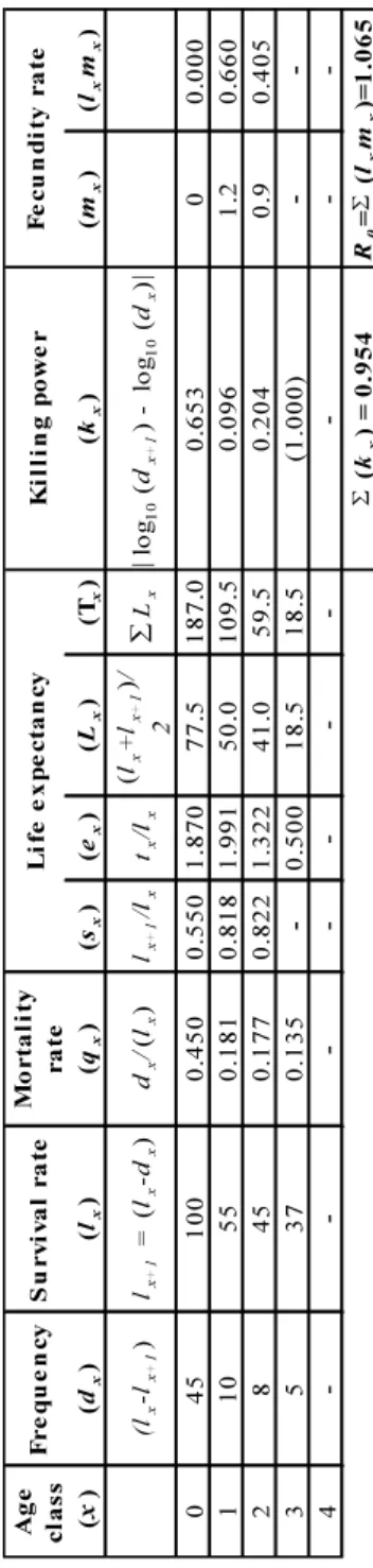
3.1 Presentation of life tables

Life tables were primarily introduced to biologists to determine the lifetime of insects [80]. They are constructed from observations of age structure of animals sampled as dead (dx) in paleobiological contexts or/and as alive (lx) in ecological field analyses.

This approach was popularized to estimate age-specific survival rates of current mam-mal and bird populations by Deevey [81]. Two main models are employed according the sampling and the nature of the population : age-specific or dynamic (horizontal or longitudinal) ; static or time-specific (vertical or transversal).

The “dynamic” or “cohort” life tables consist in following all the individuals of a single cohort in a population from birth to death. The method depends on the recapture of marked individuals for mobile species and individuals should be monitored from birth to death. This “horizontal/longitudinal” life table technique is not well suited for the study of long-lived individuals and inappropriate with fossil samples. However the “static” or “time-specific” life tables are established from individuals of all ages

(14)

belonging to different cohorts. Then “vertical/transversal” life tables represent random samples of individuals and their distribution should reflect the whole population. In this study we will focus on the latter that has been fully or partly used in both mammalian paleontological and archaeological contexts [1, 2, 5, 82-89, 36, 41, 43, 90-91].

Most importantly, time specific model allows taking into account multiple fossil de-posits through time. However, the validity of the life table analysis requires some strong assumptions to be fulfilled. For example, vertebrate population analyses have involved a female-dominant model, such that only demographic parameters of females are considered [92]. However it is widely accepted that male survival does not affect the population growth rate of most natural mammalian populations. Consequently the model can be used in a legitimate and appropriate manner assuming a balanced sex-ratio at birth and measuring the fecundity rate as the number of daughters per female as half the number of offspring produced alive at birth by a female of a given age. A stationary age structure through time is required except for the time-specific model, with constant survival and fecundity rates for the different cohorts [93-97]. It is also assumed that the age structure of the sample corresponds to a local popu-lation in the absence of immigration and emigration, that is to say that migration flows are random and did not modify the sample [98, 99]. We should keep in mind that in current ecological studies these strict assumptions are unlikely to be met in any population of wild mammals because opportunities to monitor entire cohorts for long periods of time are unlikely [100-102]. Time-specific life table and indices are explained below (see Table 1 for example) :

• (x) refers either to “age interval” or “age class” (in months, year or any time interval). There is often confusion between them. Let’s retain that according to Caswell [103] the former begins at 0 and the latter at 1.

• (dx) refers to the proportion of individuals of the whole cohort(s) dying between

age x and x + 1. This is typically the MNI. It can be derived from the variable (lx) series by :

dx= (lx− lx+1)

• (lx) refers to cumulated survivorship and corresponds to the fraction of a cohort

that survives to an age interval x. The first value can be expressed per 1, 100 or 1000 :

lx+1= (lx− dx)

In standardized life table with regular pooled age-class intervals (see example in Table 2) where dx is not available the calculation by algebraic relation with (sx) defined

below in the text is simply :

lx+1= sx∗ lx

As we can see in Figure 2, when lx values are plotted on a logarithmic scale (y-axis)

with standardized lifespan (x-axis), the survival curves obtained have the remarkable property of being similar for most mammal species despite the variation of their size

(15)

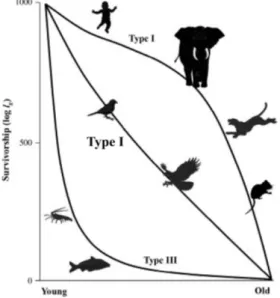
or their longevity [98]. This is also true for survival rates of other animal groups, which allows the identification of three main types of mortality. The comparison is then possible to a specific or an interspecific level. Type I, characteristic of most mammals, clearly shows that survivorship is relatively low in juveniles, becomes high and stable during adult primes, and then finally declined with a half-bell shape at old ages (senescent stage). Type II characterizes essentially small birds or raptors and is characterized by a quite constant survival over the lifetime. Type III is mainly associated with fish and marine vertebrates and shows survival rates that are low during early ages and prime ages, and then high throughout the rest of the lifetime, which generates an L-shape profile [93].

Figure 2 – Survivorship curves from stable populations (log lx) according to the zoological

group. Data are from Fernandez et al. [41] modified from Krebs [94] and Ricklefs [95].

• (qx) indicates the mortality rates during the interval x to x + 1. It is the ratio

of dxand lx:

qx= [dx/(lx)] ∗ 100

• (sx) refers to age-specific survival rate. Proportion of individuals surviving

from age x to x + 1 :

sx= [lx+1/lx] ∗ 100

• (ex) refers to life expectancy in each age class. Unlike the other columns, life

expectancy deals with the intermediate calculation of Tx(total years lived for

all individuals) and Lx(average individual number alive in age class) which are

purely intermediate step without real biological meaning. Thus life expectancy is as follow :

ex= Tx/lx

(16)

• (kx) also designated as killing power or killing factor is another measure of

mortality between successive age class. By summing individual values (P kx),

one obtains an additive index that indicates the “intensity” of mortality that may be generated by one or different factors (g. predation), calculation is as follows :

kx= | log10(dx+1) − log10(dx)|

• (mx) is the number of female offspring per female of age x (called fecundity

rate).

• (lxmx) is the contribution of a given age class to the population reproduction.

It is simply the product of lx and the mx

• (R0) is the net reproductive rate of the cohort. It corresponds to the mean

lifetime reproductive success in the population. When R0< 1 the population

is declining, meaning that animals of the cohorts are not replacing themselves. R0> 1indicates an increasing population, while R0= 1means a perfect stable

stationary population :

R0=

X lxmx

• The way to transform survival frequencies related to successive irregular age intervals and to distribute them into regular age class intervals is crucial and remains largely underused in zooarchaeological studies (see Caughley [98] for a full treatment of standardization). We present here how to pool age classes in regular intervals and calculate age-specific survival rates (sx). Starting from

an original life table data of fossil H. refossa (Geula, Israel, [90]), we detailed in the Table 2, a step-by-step example.

(17)

Table 1 – Example of time-specific life table based on the collection of dead animals with the key demographic parameters (see details for meaning and calculation in text).

(18)

Table 2 – Example of original life table of Hystrix refossa (A) and standardization with regular age classes intervals with calculation of survival rates. (Data from Monchot et al. [90].)

(19)

3.2 Presentation of Leslie matrices

In paleobiological contexts, Leslie matrices have only been used or even mentioned until recently in a very few works ([43], [90], [104-108]). However, they have become a standard in population ecology ([103], [109]) due to their long-established use since the works of Bernardelli [110], Lewis [111] and the most accomplished studies of age-structured model of population growth by Leslie [112, 113]. Later on, Lefkovitch [114] introduced developmental stages rather than ages and Usher [115] developed a size-structured model. We present here the simplest matrix projection model also called Lewis-Leslie :        m0 m1 m2 · · · m12 S0 0 0 · · · 0 0 S1 0 · · · 0 ... ... ... ... 0 0 0 0 S11 0        A ∗        n0(t) n1(t) n2(t) ... n12(t)        n(t) =        n0(t + 1) n1(t + 1) n2(t + 1) ... n12(t + 1)        n(t + 1)

Matrix A is constructed with the same age-specific fecundity rates (m0, m1. . . ) as

in the life tables. The diagonal of the matrix contains age-specific survival rate (S0,

S₁. . . ) corresponding to the values of sx in our life tables. The state vector n(t) is

derived from the (lx) as the fraction of the total number of individuals. The projection

of the matrix, with the state vector n(t) gives a new vector n(t + 1), which is simply the new number of individuals in each age interval at the next succeeding census of the projection interval such as : An(t) = n(t + 1)

In addition to the above, the model is based on three strong assumptions :

• age is a discrete variable where the first value is 0, is divided into age classes numbered from 1 to n ;

• the time is regarded as a discrete variable. The time is denoted t, and the time step projection is t + 1 ;

• the time step projection is strictly equal to the duration of each age class interval. This implies that from t to t + 1 all surviving individuals move to the next age class.

Let’s give an example of this theoretical model starting from the demographic para-meters of E. achenheimensis recovered on the natural middle Pleistocene swallow-hole of Romain-la-Roche (Doubs, France) [43]. Using the software PopTools developed by Hood [116], we first entered data into a pre-breeding1 _{Leslie matrix [102]. In the}

Figure 3-A, the first line of our matrix contains the fecundity rates multiplied by juvenile survival (i.e. S0), and the survival rates from S1onward are entered on the

sub-diagonal in order to be multiplied by the state vector. The matrix returns the dominant eigenvalue (λ) also known as the asymptotic growth rate (λ) and r, the exponential or continuous growth rate, which is simply the natural logarithm of λ, in

1. This is the basic model used for mammals where cohorts are censuse just before they breed as opposed to post-breeding model (see details in Caswell [103]).

(20)

our example r = ln(0.9869) = −0.0132_{. Decreasing populations are characterized by}

negative values of r, corresponding to lambda values less than 1. Conversely, increasing populations have positive r-values, and asymptotic growth rate greater than 1 (see details in [94]). In our example, considering λ = 0.9869 and r = −0.013, the horse population of Romain-la-Roche was likely going extinct (less than 2 individuals at t297) (Figure 3-B). In our projections, if we divide the entire population distribution

(n) at time t+1by the members of the preceding age-class, we obtain quotients that

converge to the dominant eigenvalue of the matrix, which is 0.9869. The lambda is the ratio of the population size in one year relative to that in the preceding year [97]. In our example, population changes in number by a factor of λ = 0.9869 (98.69%) from one year to the next. In other words, the entire population will decrease by more than 1% per year (0.0131%). Works on different current populations of wild Equids indicate that when they evolve in optimal conditions the λ is comprised between 1.21 and 1.26 [117-118 with λ = 1.21] ; [119 with λ = 1.26] ; [120-121 where λ = 1.22]. We should note that the early fluctuations of λ, the so-called transient dynamics, are due to initial conditions of the demographic parameters of the age distribution. For instance, in going from time t3to t4, the projection of the cohorts is of 0.9884%. If we

look now to t19including the following years, the lambda is stabilized to the dominant

eigenvalue of the matrix. The damping ratio3 _{(ρ = λ}₁_/|λ₂_|_{) describes how quickly}

the transient dynamics is stabilized after perturbation around the asymptotic growth rate regardless of population structure ; the larger the ρ (always more than 1), the quicker the population converges [102]. Surprisingly, in our example ρ = 1.245 is not very much larger than 1 suggesting that the stable size distribution is not reached very quickly.

Demographic rates in paleobiological contexts are inferred from current species, then it is of great interest to generate noise in the matrix or to explore different hypotheses by changing values such as m0, m1, S0, S1. . . In other words, how much would

λ respond to a 10 or 20% change in survival or in fecundity rates ? Elasticity4 or sensitivity analyses answer this question since they have become a standard practice in population dynamics [122-123]. Elasticity is a normalized dimensionless sensitivity as a response to a proportional perturbation. We will focus here on the former, which is easier to interpret because it is scaled to 1.

2. Then P=P0ert, where P0is the initial population, r is the continuous growth rate, and t is time. In

our example :

P _{= P}0(0.9869)t= P0ert

(0.9869)t_{= e}rt_{= (e}r₎t

0.9869 = er

3. The calculation was made with R version 3.2.3 with package “popdemo”. Theoretical details of the calculation of the damping ratio with the subdominant eigenvalue2go well beyond our paper (for details

see Caswell [103, p. 95]).

4. We will not delve into matrix formulations in detail here (see Caswell [103, Chapter 9]) and we will only focus in this study on elasticity that can be formalized such as :

eij=aijλ ∂λ

∂aij =

∂ log λ

(21)

Figure 3 – Leslie matrix with survival from 1 year of age (values in diagonal) and fecundity rates times juvenile survival (value in the first row) with the state vector (value on the right) of Equus achenheimensis (A). Time-step projections of the population with the geometric growth rate (B) and their graphical overview. (Data from Fernandez & Boulbes [43], Table 3.)

(22)

Figure 4 – (A) changing vital rates from the original Leslie matrix of Hystrix refossa ; (B) perturbation analysis with elasticity Matrix ; (C) proportional effect of changes on survival and fecundity rates (see explanation in text ; data from Monchot et al. [90])

Let’s take the matrix of the fossil porcupine H. refossa (Figure 4-A) from the natural shelter of Geula cave (Mount Carmel, Israel) [124]. The dominant eigenvalue of the matrix is λ = 1.0001 showing a perfect stability through the deposits of the different cohorts of porcupines and suggesting a non-impacted population. Suppose that we increase by 20% the first survival rate S0=0.525 being now 0.630, then new growth

rate is 1.0391 (increased by 3.9%). Let’s do the same with the original fecundity rate m1 = 0.250 being now 0.300 corresponding to new λ = 1.0333 (increased by

3.3%). It appears that the population lambda is more sensitive to changes in the first year survivorship than to changes of fecundity rate from the first reproduction. In our example it is possible to display elasticity values in a new matrix to each of the matrix entry (Figure 4-B). The results clearly show that a given change in young

(23)

and adult survival would have a greater effect on λ than fecundity (Figure 4-C). This perturbation analysis indicates that a 1% increase in the survivorship of the first age class leads to increase the lambda by 0.21%, ten times more than the corresponding fecundity that would lead to increase the λ by 0.02%. In our field, it is not trivial to consider this approach because it gives trends on how λ evolves for different species. To summarise, and as if we were in the cave counting the last individual, elasticity of H. refossa indicates that the most critical vital rate to impact the age structure was the survivorship of young and adults. This is also the case in modern populations of large herbivores [125]. Elasticity analysises are consequently very powerful in wildlife management to identify what demographic rates are the most inferential in the po-pulation dynamics and the evolution of life histories (see for example r or K selection theory : [126-127]).

4 Conclusion

Giving step-by-step examples we showed that estimating dental individual ages, and then, establishing their distribution in appropriate age class intervals according to prediction error of median age provide an efficient way to construct mortality curves. We questioned the two dominant theoretical types of mortality, attritional vs catas-trophic that are usually considered as key components to describe fossil age structures in zooarchaeological literature. With minor exceptions, and whatever the methodo-logical approach, all fossil age structures are submitted to taphonomic biases (s.l. natural, anthropic or carnivore modifications) so that only a fraction of the original paleontological or archaeological assemblage is recovered. Furthermore if the deposit conditions (i.e. unique or multiple assemblage) are not known precisely, then U- and L-shape mortality and especially intermediate patterns cannot accurately be associated to specific human/carnivore food behaviour tactics. For example does it make sense to interpret different fossil age structures mixed through time that are not consequently related to one single population of predators ? We examined in detail how the use of time specific model provided standard demographic parameters to assess mammalian mortality.

The remarkable properties of life table components (see above lx, qx, sx, ex, kx, R0,

etc.) offer multiple possibilities to compare fossil age structures between species from different zoological groups and contexts. Moreover, current mammal life tables whose causes of death are known as well as demographic parameters may help control for some biases in the fossil assemblages. Finally, on the basis of different case studies we presented a simple Leslie matrix model that admit multiple cohorts and allow to answer central issues such as is the sum of their different age structures reflect a sta-tionary and stable population at a given time ? Which demographic parameters are the most sensitive to the final state of the population ? This prerequisite is essential in natural paleontological contexts (carnivore dens, pitfall/aven, etc.) as well as in anthropic sites. We showed that Leslie matrices gave both the picture of the initial fossil sample and the projection of the entire population according to original demo-graphic parameters. This may seem counterintuitive in our field but this is the way

(24)

to characterize the state of a population and its viability in a population dynamics context.

Finally, we showed that the model could provide suppleness by performing perturba-tion analysis (e.g. sensitivity/elasticity) in order to identify in each age class which demographic component (survivorship, fecundity) was potentially the most sensitive to influence the population growth.

To conclude, the review of methodological different approaches in zooarchaeological studies indicates that our community failed to normalize mortality patterns for Pleis-tocene mammal species. It appeared that all paleobiological contexts are submitted to multiple taphonomical biases including natural or animal modifications that af-fect original samples size. With few exceptions with clear evidence of unique deposit and contemporaneity of all individuals, assumption of different cohorts/individuals through time should be made to interpret mammalian age structures. In this way current ecological models such as life table and Leslie matrices are appropriate to estimate crucial demographic parameters of fossil age structures.

References

[1] B. Kurtén, Age groups fossil in mammals. Societas Scientiarum Fennica, Commentationes Biologicae, XIII, 1-6, 1953.

[2] B. Kurtén, On the variation and population dynamics of fossil and recent mammal populations. Acta Zoologica Fennica, 76, 5-122, 1953.

[3] B. Kurtén, Population dynamics : a new method in palaeontology. Journal of Paleontology. 28, 286-292, 1954.

[4] B. Kurtén, Life and death of the Pleistocene Cave Bear. Acta Zoologica fennica, 95, 1-59, 1958 [5] B. Kurtén, Variation and dynamics of a fossil antelope population. Paleobiology, 9, 62-69, 1983 [6] C. Reher, G. C. Frison, The Vore site, 48CK302, a stratified buffalo jump in the Wyoming Black Hills. Plains Anthropologist, 16, 1-190, 1980.

[7] A. Grant, “The use of tooth wear as a guide to the age of domestic Ungulates”, in Ageing and sexing ani-mal bones from archaeological sites, eds. B. Wilson, C. Grigson, S. Payne, British Archaeological Reports, International Series, 109, Oxford, p. 91-108.

[8] B. Wilson, C. Grigson, S. Payne, Ageing and sexing animal bones from archaeological sites, Ed. British Archaeological Reports, International Series, 109, Oxford, 268 p., 1983.

[9] H. Koike, N. Ohtaishi, Prehistoric hunting pressure estimated by the age composition of excavated Sika deer (Cervus nippon) using the annual layer of tooth cement. Journal of Archaeological Science, 12, 443-456, 1985.

[10] M. C. Stiner, The use of mortality patterns in archaeological studies of hominid predatory adaptations. Journal of Anthropological Archaeology, 9, 305-351, 1990.

[11] M. C. Stiner, Human Predator and Prey Mortality. Westview Press, Boulder, 276 p., 1991.

[12] M. C. Stiner, Honor Among Thieves : a Zooarchaeological Study of Neandertal Ecology, Princeton University Press, Princeton, 447 p., 1994.

[13] T. E. Steele, Variation in mortality profiles of Red Deer (Cervus elaphus) in Middle Palaeolithic assemblages from Western Europe. International Journal of Osteoarchaeology, 14, 307-320, 2004. [14] S. Payne, Kill-off Patterns in Sheep and Goats : the Mandibles from Aşvan Kale. Anatolian Studies, 23, 281-303, 1973.

[15] P. J. Munson, Age-correlated Differential Destruction of Bones and its Effect on Archaeological Mor-tality Profiles of Domestic Sheep and Goats. Journal of Archaeological Science, 27, 391-407, 2000.

(25)

[16] V. P. W. Lowe, Teeth as indicators of age with special reference to Red Deer (Cervus elaphus) of known age from Rhum. Journal of Zoology, 152, 137-153, 1967.

[17] P. H. Riglet, « Contribution à l’étude de l’âge du Cerf élaphe (Cervus elaphus) », Thèse de l’École nationale vétérinaire d’Alfort, 104, 75 pages, 1977.

[18] J. P. Briot, D. Voilquin, « Contribution à l’étude comparative de l’usure dentaire en fonction du biotope chez Cervus elaphus (Cerf noble) », Thèse de 3éme cycle, Université de Nancy, 230 pages, 1986. [19] M. Paulus, « Contribution à l’étude de l’âge du Chevreuil (Capreolus capreolus) d’après les dents », Thèse de l’École nationale vétérinaire d’Alfort, n° 43, 105 pages, 1973.[20] J. P. Mauries, « Contribution à l’étude de la biologie et du comportement du Chevreuil (Capreolus capreolus), Thèse de l’École nationale vétérinaire d’Alfort, 79, 118 pages, 1979.

[21] G. Van Laere, J. M. Boutin, J. M. Gaillard, Estimation de l’âge chez le Chevreuil (Capreolus capreolus) par l’usure dentaire : Test de fiabilité sur des animaux marqués. Gibier Faune Sauvage, 6, 417-426, 1989. [22] M. A. J. Couturier, Le chamois, Editions Arthaud, Grenoble, 855 pages, 1938.

[23] M. A. J. Couturier, Détermination de l’âge du Bouquetin des Alpes (Capra aegagrus ibex ibex) à l’aide des dents et des cornes. Mammalia, 26, 453-461, 1962.

[24] C. A. Spinage, Geratodontology and horn growth of the Impala (Aepyceros melampus). Journal of Zoology, 164, 209-225, 1971.

[25] C. A. Spinage, African Ungulate life tables. Ecology, 53, 645-652, 1972.

[26] R. G Klein, C. Wolf, L. G. Freeman, K. Allwarden, The use of dental crown heights for constructing age profiles of red deer and similar species in archaeological samples. Journal of Archaeological Science, 8, 1-31, 1981.

[27] R. G. Klein, Age (mortality) profiles as means of distinguishing hunted species from scavenged ones in Stone Age archaeological sites. Paleobiology, 8, 151-158, 1982a.

[28] R. G. Klein, Patterns of ungulates mortality profiles from Langebaanweg (Early Pliocene) and Eland-sfontein (Middle Pleistocene), south western Cape province, South Africa. Annals of the South African Museum, 90, 49-94, 1982b.

[29] R. G. Klein, K. Allwarden, C. Wolf, “The calculation and interpretation of ungulate age profiles from dental crown heights”. In Hunter-gatherer economy in prehistory : a european perspective, eds. G. Bailey, Cambridge University Press, Cambridge, 47-57, 1983.

[30] R. G. Klein, K. Cruz-Uribe, The computation of ungulates age (mortality) profiles from dental crown heights. Paleobiology, 9, 70-78, 1983.

[31] R. G. Klein, G. Avery, K. Cruz-Uribe, T. E. Steele (2007) - The mammalian fauna associated with an archaic hominin skullcap and later Acheulean artifacts at Elandsfontein, Western Cape Province, South Africa. Journal of Human Evolution, 52, 164-186, 2007.

[32] D. Gifford-Gonzalez, “Examining and refining the quadratic crown height method of age estimation”. InHuman predators and prey mortality, ed. M. C. Stiner, Westview press, Boulder, p. 41-78, 1991. [33] A. Pike-Tay, C. A. Morcomb, M. O’Farrell, Reconsidering the quadratic crown height method of age estimation for Rangifer from archaeological sites. Archaeozoologia, 11, 145-174, 2000.

[34] P. Fernandez, « Etude paléontologique et archéozoologique des niveaux d’occupations moustériens au Bau de l’Aubesier (Monieux, Vaucluse) : implications biochronologiques et palethnologiques », Thèse de Doctorat, Université Claude Bernard Lyon I, 286 pages, 2001.

[35] T. E. Steele, D. Weaver, The modified triangular graph : a refined method for comparing mortality profiles in archaeological samples. Journal of Archaeological Science, 29, 317-322, 2002.

[36] P. Fernandez, S. Legendre, Mortality curves for horses from the Middle Palaeolithic site of Bau de l’Au-besier (Vaucluse, France) : methodological, palaeo-ethnological, and palaeoecological approaches. Journal of Archaeological Science, 30, 1577-1598, 2003.

[37] M. A. Levine, « Archaeo-Zoological Analysis of Some Upper Pleistocene Horse Bone Assemblages in Western Europe », PhD Thesis, University of Cambridge, 372 pages, 1979.

[38] R. R. Sokal, F. J. Rohlf, Biometry, the principles and practice of statistics in biological research, Freeman and Co, New-York, 859 pages, 1981.

(26)

[39] P. Fernandez, De l’estimation de l’âge individuel dentaire au modèle descriptif des structures d’âge des cohortes fossiles : l’exemple des Equidae et du time-specific model en contextes paléobiologiques pléis-tocènes. Bulletin de la Société préhistorique française, 106, 5-14, 2009.

[40] L. Gourichon « Faune et saisonnalité. L’organisation temporelle des activités de subsistance dans l’Epipaléolithique et le Néolithique précéramique du Levant nord (Syrie) », Thèse de doctorat, Université Lumière-Lyon 2, 755 pages, 2004.

[41] P. Fernandez, J. L. Guadelli, P. Fosse, Applying dynamics and comparing life tables for Pleistocene Equidae in anthropic contexts (Bau de l’Aubesier, Combe Grenal) and Carnivore (Fouvent) contexts with modern feral Horse populations (Akagera, Pryor Mountain). Journal of Archaeological Science, 33, 176-184, 2006.

[42] S. Q. Zhang, Z. Y., Zhang, X. Gao, Mortality profiles of the large herbivores from the Lingjing Xuchang Man Site, Henan Province and the early emergence of the modern human behaviors in East Asia. Chinese Science Bulletin, 54, 3857-3863, 2009.

[43] P. Fernandez, N. Boulbes, Analyse démographique des cohortes fossiles du cheval pléistocène moyen de Romain-la-Roche (Doubs, France), Revue de Paléobiologie, Genève, 29, 771-801, 2010.

[44] Z. Y. Li, S. Q. Zhang, Y. Zhang, X. Gao, Mortality Curves for Horses (Equus caballus) from the Lingjing Site, Henan Province. Acta Anthropologica Sinica, 30, 45-54, 2011.

[45] M. A. Julien, F. Rivals, J. Serangeli, H. Bocherens, N. J. Conard, A new approach for deciphering between single and multiple accumulation events using intra-tooth isotopic variations : Application to the Middle Pleistocene bone bed of Schöningen 13 II-4. Journal of Human Evolution, 89, 114-128, 2015. [46] A. R. Millard, « A Bayesian Approach to Ageing Sheep/Goats from Toothwear », Recent Advances in Ageing and Sexing Animal Bones 9th ICAZ Conference, ed. D. Ruscillo Durham, 145-154, 2002. [47] L. W. Konigsberg, D. Holman, « Estimation of age at death from dental emergence and implications for studies of prehistoric somatic growth », Human Growth in the Past, eds R. D. Hoppa, C. M. Fitzgerald, Cambridge University Press, 264-289, 1999.

[48] J. P. Bocquet-Appel, C. Masset, Farewell to palaeodemography. Journal of Human Evolution, 11, 321-333, 1982.

[49] P. Fandos, J.F. Orueta, Y. Aranda, Tooth wear and its relation to kind of food : the repercussion on age criteria in Capra pyrenaica. Acta Theriologica, 38, Bielowiza, 93-102, 1993.

[50] M. Fortelius, N. Solounias, Functional characterization of Ungulate molars using the abrasion-attrition wear gradient : a new method for reconstructing paleodiets. American Museum Novitates, 3301, 1-36, 2000. [51] F. Rivals, N. Solounias, M. C. Mihlbachler, Evidence for geographic variation in the diets of late Pleistocene and early Holocene Bison in North America, and differences from the diets of recent Bison. Quaternary Research, 68, 338-346, 2007.

[52] N. Solounias, G. M. Semprebon, Advances in the reconstruction of Ungulate ecomorphology with application to early fossil Equids. American Museum Novitates, 3366, 1-49, 2002.

[53] F. Rivals, N. Solounias, Differences in tooth microwear of populations of caribou (Rangifer tarandus, Ruminantia, Mammalia) and implications to ecology, migration, glaciations and dental evolution. Journal of Mammalian Evolution, 14, 182-192, 2007.

[54] F. Rivals, M. A. Julien, M. Kuitems, T. Van Kolfschoten, J. Serangeli, D. G. Drucker, H. Bocherens, N. J. Conard, Investigation of equid paleodiet from Schöningen 13 II-4 through dental wear and isotopic analyses : Archaeological implications. Journal of Human Evolution, 89, 129-137, 2002.

[55] G. Haynes, Proboscidean die-offs and die-outs : age profiles in fossil collections, Journal of Archaeolo-gical Science, 14, 6, 659-668, 1987.

[56] C. A. Spinage, A review of age determination of Mammals by means of teeth, with special reference to Africa, East African Wildlife Journal, 11, 165-187, 1973.

[57] R. L. Lyman, On the analysis of Vertebrate mortality profiles : sample size, mortality type and hunting pressure. American Antiquity, 52, 125-142, 1987.

[58] R. L. Lyman, “Taphonomy of Cervids killed by the 18 may 1980 volcanic eruption of Mount St. Helens, Washington”, In Bone modification, eds R. Bonnischsen, M. Sorg, Center for the Study of the First Americans, University of Maine, 149-167, 1989.

(27)

[60] D. A. Byers, B. L. Hill, Pronghorn Dental Age Profiles and Holocene Hunting Strategies at Hogup Cave, Utah. American Antiquity, 74, 299-321, 2009.

[61] T. E. Steele, Comparing methods for analysing mortality profiles in zooarchaeological and paleontolo-gical samples. International Journal of Osteoarchaeology, 15, 1-17, 2005.

[62] H. J. Greenfield, The Paleoeconomy of the Central Balkans (Serbia) : A Zooarchaeological Perspective on The Late Neolithic and Bronze Age (ca. 4500-1000 B.C.). Part I and II, BAR International Series, Oxford. 513 pages, 1986.

[63] H. J. Greenfield, The origins of milk and wool production in the Old World. Current Anthropology 29, 573-593, 1988.

[64] J. D. Vigne, D. Helmer, Was milk a “secondary product” in the Old World neolithisation process ? Its role in the domestication of cattle, sheep and goats. Anthropozoologica, 47, 9-40, 2007.

[65] J. E. Brochier, The use and abuse of culling profiles in recent zooarchaeological studies. Some metho-dological comments on “frequency correction” and its consequences. Journal of Archaeological Sciences, 40, 1416-1420, 2013.

[66] M. C. Stiner, The use of mortality patterns in archaeological studies of hominid predatory adaptations. Journal of Anthropological Archaeology, 9, 305-351, 1990.

[67] T. E Steele, T. D. Weaver, The modified triangular graph : a refined method for comparing mortality profiles in archaeological samples. Journal of Archaeological Science, 29, 317-322, 2002.

[68] T. D Weaver, R. H. Boyko, T. E Steele, Cross-platform program for likelihood-based statistical com-parisons of mortality profiles on a triangular graph. Journal of Archaeological Science, 38, 2420-2423, 2011. [69] E. Discamps, S. Costamagno, Improving mortality profile analysis in zooarchaeology : a revised zoning for ternary diagrams, Journal of Archaeological Science, 58, 62-76, 2015.

[70] B. J. Nimmo, Population Dynamics of a Wyoming Pronghor Cohort from the Eden-Farson Site, 48SW304. Plains Anthropologist, 16, 285-288, 1971.

[71] C. N. G. Trueman, A. K. Behrensmeyer, N. Tuross, S. Weiner, Mineralogical and compositional changes in bones exposed on soil surfaces in Amboseli National Park, Kenya : diagenetic mechanisms and the role of sediment pore fluids. Journal of Archaeological Science, 31, 721-739, 2004

[72] J. L. Guadelli, La gélifraction des restes fauniques. Expérimentation et transfert au fossile. Annales de Paléontologie, 94, 121-165, 2008.

[73] P. Andrews, J. Cook, Natural Modifications to Bones in a Temperate Setting. Man, 20, new series, 675-691, 1985.

[74] L. R Binford, Nunamiut ethnoarchaeology, Academic Press, New York, 509 pages, 1978.

[75] H. T Bunn, L. E Bartram, E. M. Kroll, Variability in bone assemblage formation from Hadza hunting, scavenging, and carcass processing. Journal of Anthropological Archaeology, 7, 412-457, 1988.

[76] R. J. Blumenschine, “Prey size and age models of prehistoric hominid scavenging : test cases from the Serengeti”, In Human predators and prey mortality, ed. M. C. Stiner, Westview press, Boulder, 122-147, 1991.

[77] C. W. Marean, Hunter/gatherer foraging strategies in tropical grasslands : model building and testing in the East African Middle and Late Stone Age. Journal of Anthropological Archaeology, 16, 189-225, 1997. [78] M. A. Levine, “The use of crown height measurements and eruption-wear sequences to age Horse teeth”, InAgeing and sexing animal bones from archaeological sites, eds B. Wilson, C. Grigson, S. Payne, British Archaeological Reports, International Series, , 109, Oxford, 223-250, 1982.

[79] M. A. Levine, “Mortality models and the interpretation of Horse population structure”, In Hunter-gatherer economy in Prehistory : a European perspective, ed G. Bailey, Cambridge University Press, Cam-bridge, 23-46, 1983.

[80] R. Pearl, J. R. Miner, Experimental studies on the duration of life. XIV. The comparative mortality of certain lower organisms. The Quaterly Review of Biology, 10, 60-79, 1935.

[81] E. S. Deevey, Life tables for natural populations of animals, The Quaterly Review of Biology, 22, 283-314, 1947.

[82] L. Van Valen, Selection in natural populations : Merychippus primus, a fossil Horse, Nature, 4873, 197, 1181-1183, 1963.

(28)

[83] L. Van Valen, Age in two fossil Horse populations, Acta Zoologica, vol. 45, 93-106, 1964.

[84] L. Van Valen, Selection in natural populations. III. Measurement and estimation, Evolution, 19, 514-528, 1965.

[85] M. R. Voorhies, Taphonomy and population dynamics of an Early Pliocene Vertebrate fauna, Knox County, Nebraska. Contributions to Geology, Special Paper n° 1, University of Wyoming, Laramie, 1-69, 1969.

[86] J. D. Speth, Bison kills and bone counts : decision making by ancient hunters. University of Chicago Press, Chicago, 227 pages, 1983.

[87] G. C. Frison, The Carter/Kerr-Mcgee Paleoindian Site : CulturalResource Management and Archaeo-logical Research. American Antiquity 49, 288-314, 1984.

[88] H. Koike, N. Ohtaishi, Estimation of prehistoric hunting rates based on the age composition of Sika Deer (Cervus nippon). Journal of Archaeological Science, 14, 251-269, 1987.

[89] M. C. Mihlbachler, Demography of late Miocene rhinoceroses (Teleoceras proterum and Aphelops malacorhinus_{) from Florida : linking mortality and sociality in fossil assemblages. Paleobiology, 29,} 412-428, 2003.

[90] H. Monchot, P. Fernandez, J. M. Gaillard, Palaeodemographic analysis of a fossil porcupine (Hystrix refossaGervais, 1852) population from the Upper Pleistocene site of Geula Cave (Mount Carmel, Israel). Journal of Archaeological Science, 39, 3027-3038, 2012.

[91] M. Price, J. Wolfhagen, E. Otárola-Castillo, Confidence intervals in the analysis of mortality andsur-vivorship curves in zooarchaeology. American Antiquity, 81, 157-173, 2016.

[92] J. M. Gaillard, A. Loison, C. Toïgo, “Variation in life history traits and realistic population models for wildlife management. The case of ungulates”, In Animal Behavior and Wildlife Conservation, eds. M. Festa-Bianchet, M. Apollonio, Island Press, Washington, 115-132, 2003.

[93] G. Caughley, Mortality patterns in mammals. Ecology, 47, 906-918, 1966.

[94] C. J. Krebs, Ecology : the experimental analysis of distribution and abundance. Benjamin Cummings, San Francisco, 695 pages, 2001.

[95] R. E. Ricklefs, The economy of nature, Freeman and Co, New-York, 678 pages, 1997. [96] R. E. Ricklefs, G. L. Miller, Ecology, fourth ed. Freeman, New York, 822 pages, 1999.

[97] A. R. E. Sinclair, The natural regulation of buffalo populations in East Africa. III. Population trends and mortality. East African Wildlife Journal, 12, 185-200, 1974.

[98] G. Caughley, Analysis of Vertebrate Populations, Caldwell, New Jersey, 234 pages, 1977.

[99] G. Caughley, A. R. E. Sinclair, Wildlife Ecology and management, Blackwell Science, Cambridge, Massachusetts, USA, 334 pages, 1994.

[100] J. M. Gaillard, M. Festa-Bianchet, N. Yoccoz, Population dynamics of large herbivores : variable recruitment with constant adult survival. Trends in Ecology and Evolution, 13, 58-63, 1998.

[101] D. R. McCullough, F. W. Weckerly, P. I. Garcia, R. R. Evett, Sources of inaccuracy in black-tailed deer herd composition. Journal of Wildlife Management, 58, 319-329, 1994.

[102] G. E. Menkens, M. S. Boyce, Comments on the use of time-specific and cohort life tables. Ecology, 74, 2164-2168, 1993.

[103] H. Caswell, Matrix Population Models : Construction, Analysis and Interpretation, Sinauer Associates, Sunderland, Massachusetts, 722 pages, 2001.

[104] G. Rodríguez-Gómez, A. Mateos, J. A. Martín-González, R. Blasco, J. Rosell, J. Rodríguez, Discon-tinuity of Human Presence at Atapuerca during the Early Middle Pleistocene : A Matter of Ecological Competition ? PLoS ONE 9(7) : e101938. doi :10.1371/journal.pone.0101938, 2014a.

[105] G. Rodríguez-Gómez, J. A. Martín-González ; I. Goikoetxea, A. Mateos ; J. Rodríguez, “A New Mathe-matical Approach to Model Trophic Dynamics of Mammalian Palaeocommunities. The Case of Atapuerca-TD6” In Mathematics of Planet Earth. Proceedings of the 15th Annual Conference of the International Association for Mathematical Geosciences, Lecture Notes in Earth System Sciences, (Apéndice G), Ed. Springer, ISSN 2193-8571, ISBN 978-3-642-32407-9, Madrid, 739-745, 2014b.

[106] J. A. Martín González, A. Mateos, G. Rodríguez-Gómez, J. Rodríguez, “Fitting a Survival Model to Describe the Age Structure of Fossil Populations”. XVII World UISPP Congress 2014, Burgos, p. 731, 2014.

(29)

[107] J. A. Martín González, A. Mateos, G. Rodríguez-Gómez, J. Rodríguez, A parametrical model to des-cribe a stable and stationary age structure for fossil populations. Quaternary International, http ://dx.doi.o rg/10.1016/j.quaint.2016.01.038. (2016, in press).

[108] G. Rodríguez-Gómez, « Modelización de la disponibilidad de recursos tróficos para las poblaciones paleolíticas de cazadores-recolectores », Phd, Universitat Rovira i Virgili, Tarragona, 289 pages, 2015. [109] N. Keyfitz, H. Caswell, Applied mathematical demography, Third Ed., Springer, New York, 555 pages, 2005.

[110] H. Bernardelli, Population waves. Journal of the Burma Research Society, 31, 1-18, 1941. [111] E. G. Lewis, On the generation and the growth of a population. Sankhya 6, 93-96, 1942.

[112] P. H. Leslie, On the use of matrices in certain population mathematics. Biometrika, 33, 183-212, 1945. [113] P. H. Leslie, Some further notes on the use of matrices in population mathematics. Biometrika, 35, 213-245, 1948.

[114] L. P. Lefkovitch, The study of population growth in organisms grouped by stages. Biometrics, 21, 1-18, 1965.

[115] M. B. Usher, A Matrix Approach to the Management of Renewable Resources, with Special Reference to Selection Forests. Journal of Applied Ecology 3, 2, 355-367, 1966.

[116] G. M. Hood, PopTools version 3.0.6. Available on the internet, 2008. URL http ://www.cse.csiro.au/po ptools, 2008.

[117] L. L. Eberhardt, Population projections from simple models. Journal of Applied Ecology, 24, 103-118, 1987.

[118] R. A. Garrott., L. Taylor, Dynamics of a Feral Horse Population in Montana. The Journal of Wildlife Management, 54, 4, 603-612, 1990.

[119] P. Duncan, Horses and Grasses. The Nutritional Ecology of Equids and Their Impacts on the Ca-margue. Ecological Studies, Verlag, New York, 1-287, 1992.

[120] E. Z. Cameron, W. L. Linklater, E. O. Minot & K. J. Stafford, Population dynamics 1994-98, and ma-nagement, of Kaimanawa wild horses. Science for Conservation, Department of Conservation, Wellington, New Zealand, 171, p. 1-165, 2000.

[121] M. J. Walter, The Population Ecology of Wild Horses in the Australian Alps. Phd Thesis, Applied Ecology Research Group, ACT 2601, University of Canberra, p. 1-179, 2002.

[122] H. Caswell, R. J. Naiman, R. Morin, Evaluating the consequences of reproduction in complex salmonid life cycles. Aquaculture, 43, 123-134, 1984.

[123] H. De Kroon, A. Plaisier, J.M. van Groenendael, H. Caswell, Elasticity : the relative contribution of demographic parameters to population growth rate. Ecology 67, 1427-1431, 1986.

[124] H. Monchot, P. Fernandez, J.M. Gaillard, Palaeodemographic analysis of a fossil porcupine (Hystrix refossaGervais, 1852) population from the Upper Pleistocene site of Geula Cave (Mount Carmel, Israel). Journal of Archaeological Science, 39, 9, 3027-3038, 2012.

[125] J. M. Gaillard, M. Festa-Bianchet, N. Yoccoz, Population dynamics of large herbivores : variable recruitment with constant adult survival. Trends in Ecology & Evolution, 58-63, 1998.

[126] E. R. Pianka, On r and K selection. American Naturalist,104, 940, 592-597, 1970.

[127] M. S. Boyce, Restitution of r- and K-Selection as a Model of Density-Dependent Natural Selection, Annual Review of Ecology and Systematics, 15, 427-447, 1984.

(30)

Préface

Jean-Philip Brugal i

1 Des TaphonomieS. Une introduction

Jean-Philip Brugal 1

1 Contexte . . . 1

2 Buts de la taphonomie . . . 4

3 Quels matériaux et objets d’étude ? . . . 7

4 Gisements et accumulations . . . 8

5 Altérations, destructions, modifications. . . 10

6 Conclusion . . . 14

I

Taphonomie et diagenèse

21

2 Modifications de structure et de composition des biominéraux phos-phatés des vertébrés Yannicke Dauphin, Alain Denis 23 1 Os et dents actuels : références . . . 24

2 Os et dents actuels soumis à la prédation . . . 34

3 Os et dents fossiles . . . 34

3 Le cas des « coquillages » Jean-Pierre Cuif, Yannicke Dauphin 45 1 Introduction . . . 45

(31)

530

2 Références actuelles : mollusques et coraux . . . 47

3 L’altération des structures calcaires minéralisées biogéniques . . . 64

4 Taphonomie expérimentale . . . 76

5 Conclusions . . . 77

Encart 1. – Évolution texturale et minéralogique de la coquille d’œuf d’autruche par chauffe Loïc Ségalen, Alain Person 82 1 Introduction . . . 82

2 Structure de la coquille . . . 83

3 Expérience de chauffe . . . 84

4 Sols, sédiments et biominéraux phosphatés : expériences in vitro Yannicke Dauphin, Pierre Massard 89 1 Introduction . . . 89

2 Expérimentations in vitro : données générales . . . 90

3 Mise en place d’une expérience in vitro sur les dents de Sus scrofa . . . 92

4 Attaque par la solution d’acide acétique HCO2CH3seul à 5*10-3 M . . . 94

5 Attaque par la solution d’acide oxalique H2C2O4 seul à 5*10-3 M . . . 97

6 Attaque par le mélange équimolaire acide oxalique – acide acétique . . . 99

7 Attaque par les extraits solubles du sol forestier . . . 101

8 Comparaison avec des fossiles . . . 102

5 Sols, sédiments et biominéraux phosphatés : observations Yannicke Dauphin, Pierre Massard 107 1 Introduction . . . 107

2 Les altérations pré-enfouissement ou de surface . . . 109

(32)

4 Une approche physico-chimique : les équilibres à saturation de solutions au contact des minéraux essentiels

à El Harhoura (Maroc) . . . 111

II

Taphonomie et géoarchéologie

123

6 Géoarchéologie et taphonomie des vestiges archéologiques : impacts des processus naturels sur les assemblages et méthodes d’analyse Pascal Bertran, Jean-Guillaume Bordes, Dominique Todisco, Luc Vallin 125 1 Processus de formation des sites et taphonomie archéologique : prin-cipes généraux . . . 125

2 Processus sédimentaires . . . 127

3 Processus bio-pédologiques . . . 129

4 Taphonomie archéologique : objectifs, démarche et outils disponibles . . . 130

5 État de surface du matériel lithique . . . 150

6 Conclusion et perspectives . . . 156

7 Processus géologiques de formation des sites et principaux agents taphonomiques Christiane Denys 167 1 Introduction . . . 167

2 Approches méthodologique . . . 169

3 Caractéristiques des sites fossilifères à mammifères . . . 176

4 Les réservoirs (« tanks ») naturels . . . 181

Encart 2. – Taphonomie et analyse des résidus sur les pièces lithiques Dries Cnuts, Veerle Rots 187 1 Introduction . . . 187

2 Origines des résidus . . . 188

3 Préservation des résidus . . . 189

(33)

532

III

Taphonomie et paléoanthropologie

195

8 Archéologie funéraire et taphonomie du cadavre

Henri Duday 197

1 Introduction . . . 198

2 La démonstration du caractère primaire d’une sépulture . . . 204

3 Les processus de décomposition du cadavre, ou l’archéothanatologie en quête de ses références . . . 209

4 Les transformations entre l’image originelle du dépôt et l’image obser-vée au moment de la fouille : des os qui se déplacent à l’intérieur du volume originel du cadavre . . . 218

5 Contributions des observations ostéologiques à la restitution de l’architecture funéraire . . . 223

6 Le comblement du volume intérieur au cadavre . . . 228

7 Les interactions entre le corps en décomposition, son contenant ou son support . . . 230

8 Espace vide originel / espace vide secondaire, les espaces vides « néoformés » . . . 237

9 Taphonomie et chronologie : la perception du « temps court » dans l’histoire de sépultures . . . 240

10 Quelques considérations d’ostéologie quantitative . . . 244

11 La crémation des corps . . . 248

Encart 3. –La décomposition des corps immergés dans l’eau. L’apport de l’archéothanatologie à la recherche archéologique subaquatique Vera Tiesler 254 1 La décomposition d’un corps immergé . . . 255

2 Les perturbations subies sous l’eau par les vestiges squelettisés . . . 256

3 Perspectives paléoanthropologiques . . . 257

Encart 4. –La sépulture de l’âge du fer de Karacie (Oblast de Tyumen,

Russie). Exemple de la reconstitution d’un cadavre

(34)

Encart 5. –Hécatombe dans les catacombes. Taphonomie de sépultures multiples complexes

Dominique Castex, Géraldine Sachau-Carcel, Sacha Kacki 265

1 Approche archéothanatologique classique . . . 266

2 Modalités de gestion des corps . . . 267

3 Restitution tridimensionnelle des salles et de leur contenu . . . 267

4 Évolution taphonomique des strates de cadavres . . . 268

Encart 6. –Vestiges néandertaliens, sépultures moustériennes et tapho-nomie : tout (ou presque) reste à faire. . . Bruno Maureille, William Rendu, Cédric Beauval 271 Encart 7. –Taphonomie des homininés dans les sites karstiques du dé-but du Pléistocène dans la région du Cradle of Humankind (Afrique du Sud) : le cas unique de Malapa Aurore Val 279 1 Le Cradle of Humankind . . . 279 2 Matériel étudié . . . 281 3 Méthodes . . . 281 4 Résultats . . . 282 5 Discussion . . . 285

IV

Taphonomie et paléobotanique

289

9 Archéobotanique et taphonomie Vincent Lebreton, Isabelle Thery-Parisot, Laurent Bouby, Julia Chrzavzez, Claire Delhon, Marie-Pierre Ruas 291 1 Introduction . . . 291

2 Les milieux de conservation des marqueurs archéobotaniques . . . 293

3 Taphonomie et restes botaniques : approche multiscalaire . . . 299

(35)

534

V

Taphonomie, faunes et hommes

329

10 Effets de la prédation sur la microstructure et la composition des tissus minéralisés

Yannicke Dauphin, Alain Denis, Christiane Denys 331

1 Les os . . . 332

2 Les dents . . . 335

3 Expériences de digestion in vivo et in vitro . . . 340

11 Accumulations de rapaces nocturnes et diurnes Christiane Denys 347 1 Introduction . . . 347

2 Approche méthodologique et instrumentale . . . 349

3 Exemples d’application néotaphonomiques . . . 352

4 Les catégories de prédation . . . 363

12 Taphonomie des restes ingérés par les petits carnivores Christiane Denys, David Cochard 369 1 Introduction . . . 369

2 Référentiels néotaphonomiques sur les petits mammifères carnivores . . . 371

3 Caractéristiques des coprocoenoses de petits mammifères carnivores . . . 372

4 Exemple d’étude néotaphonomique : Vulpes rueppelli, Bir Tarfawi (Égypte) . . . 379

13 Accumulations par les prédateurs non humains Jean-Baptiste Fourvel 389 1 Introduction . . . 389

2 Historique des recherches . . . 390

3 Diversité des assemblages . . . 391

(36)

14 Comportements de subsistance des hominines au Pléistocène en Afrique et en Europe Jean-Philip Brugal, Olivier Bignon-Lau, Camille Daujeard, Pierre Magniez, Anne-Marie Moigne 413 1 Introduction . . . 413

2 Hominines du Plio-Pléistocène d’Afrique (J.-Ph. B.) . . . 414

3 Hominines du Pléistocène d’Eurasie . . . 417

Encart 8. – Paléoentomologie, ichnologie et taphonomie Jean-Bernard Huchet 437 1 Introduction . . . 437

2 La préservation des insectes dans les sédiments . . . 438

3 Traces et empreintes d’insectes en contexte archéologique . . . 440

VI

Taphonomie et paléoécologie

451

15 Variations de la taille corporelle chez les ongulés pléistocènes : im-plications paléoécologiques et taphonomiques Pierre Magniez, Nicolas Boulbes, Jean-Philip Brugal 453 1 Introduction . . . 453

2 Cas d’étude . . . 454

Encart 9. – Classes de taille chez les grands mammifères Jean-Philip Brugal 472 16 Life tables and Leslie matrices for mammalian cohorts in different paleobiological contexts during the Pleistocene Philippe Fernandez, Christophe Bonenfant, Jean-Michel Gaillard, Hervé Monchot 477 1 Principles and methods : establishing mortality profiles . . . 477

(37)

536

2 Attritional and catastrophic “models” :

theoretical and practical limits . . . 479

3 Discussion : life tables and Leslie matrices . . . 481

Encart 10. – Improving eco-cultural niche estimations : the potential of archaeological faunal remains for taking biotic interactions into consideration William E. Banks 498 1 Introduction . . . 498

2 Placing archaeological cultures in an environmental context . . . 499

3 Potential cultural responses to environmental change . . . 500

4 The ecological niche . . . 501

17 The Early Pleistocene assemblages of large mammals from Orce (Baza Basin, SE Spain) : an example of reciprocal illumination bet-ween taphonomy and paleoecology Paul Palmqvist, M. Patrocinio Espigares 509 1 Introduction . . . 509

2 An overview on the Early Pleistocene localities of Orce . . . 511

3 Descriptive taphonomic attributes . . . 513

4 Osseous modification . . . 515

5 Taphonomic biases . . . 517