HAL Id: hal-03196830
https://hal.archives-ouvertes.fr/hal-03196830
Submitted on 13 Apr 2021HAL is a multi-disciplinary open access
archive for the deposit and dissemination of sci-entific research documents, whether they are pub-lished or not. The documents may come from teaching and research institutions in France or abroad, or from public or private research centers.
L’archive ouverte pluridisciplinaire HAL, est destinée au dépôt et à la diffusion de documents scientifiques de niveau recherche, publiés ou non, émanant des établissements d’enseignement et de recherche français ou étrangers, des laboratoires publics ou privés.
Finding the k Shortest Simple Paths: Time and Space
trade-offs
Ali Al Zoobi, David Coudert, Nicolas Nisse
To cite this version:
Ali Al Zoobi, David Coudert, Nicolas Nisse. Finding the k Shortest Simple Paths: Time and Space trade-offs. [Research Report] Inria; I3S, Université Côte d’Azur. 2021. �hal-03196830�
Finding the k Shortest Simple Paths: Time and Space trade-offs
∗Ali Al Zoobi and David Coudert and Nicolas Nisse Universit´e Cˆote d’Azur, Inria, CNRS, I3S, France
April 13, 2021
Abstract
The k shortest simple path problem (kSSP) asks to compute a set of top-k shortest simple paths from a source to a sink in a digraph. Yen (1971) proposed an algorithm with the best known polynomial time complexity for this problem. Since then, the problem has been widely studied from an algorithm engineering perspective. The most noticeable proposals are the node-classification (NC) algorithm (Feng, 2014) and the sidetracks-based (SB) algorithm (Kurz, Mutzel, 2016). The latest offers the best running time at the price of a significant working memory.
We first show how to speed up the SB algorithm using dynamic updates of shortest path trees resulting in a faster algorithm (SB*) with same working memory. We then propose the parsimonious SB (PSB) algorithm that significantly reduces the working memory of SB at the cost of a small increase of the running time. Furthermore, we propose the postponed node-classification (PNC) algorithm that combines the best of NC and SB. It offers a significant speed up compared to NC while using the same amount of working memory of NC.
Our experimental results on complex networks show that all of the considered algorithms have low working memory, and that the PSB algorithm is the fastest. On road networks, the SB* algorithm is the fastest (on median) among the considered algorithms, but it suffers from a large working memory. The PNC algorithm has comparable running time to SB* on road networks while using the same working memory as NC.
Keywords: k shortest simple paths; graph algorithm; space-time trade-off.
1
Introduction
The classical k shortest paths problem (kSP) aims at finding the top-k shortest paths between a pair of source and destination nodes in a graph. This problem has numerous applications in various kinds of networks (road and transportation networks, communications networks, social networks, etc.) and is also used as a building block for solving optimization problems. Let
5
D = (V, A) be a digraph, an s-t path is a sequence (s = v0, v1, · · · , vl = t) of vertices starting
with s and ending with t, such that (vi, vi+1) ∈ A for all 0 ≤ i < l. It is called simple if it has
no repeated vertices, i.e., vi 6= vj for all 0 ≤ i < j ≤ l. The weight of a path is the sum of the
weights of its arcs and the top-k shortest paths is therefore a set containing a shortest s-t path, a second shortest s-t paths, etc. until a kth shortest s-t path.
10 ∗
This work has been supported by the French government, through the UCAjedi Investments in the Future
project managed by the National Research Agency (ANR) with the reference number ANR-15-IDEX-01, the ANR project MULTIMOD with the reference number ANR-17-CE22-0016, the ANR project Digraphs with the reference number ANR-19-CE48-0013, and by R´egion Sud PACA.
Several algorithms for solving kSP have been proposed. In particular, Eppstein [8] proposed an exact algorithm that computes k shortest paths (not necessarily simple) in O(m+n log n+k)-time, where m is the number of arcs and n the number of vertices of the graph. An important variant of this problem is the k shortest simple paths problem (kSSP) introduced in 1963 by Clarke et al. [6] which adds the constraint that reported paths must be simple. This variant
15
of the problem has various applications in transportation network when paths with repeated vertices are not desired by the user. It is also a subproblem of other important problems like constrained shortest path problem, vehicle and transportation routing [16, 19, 35]. It can be applied successfully in bio-informatics [2], especially in biological sequence alignment [30] and in natural language processing [4]. For more applications, see Eppstein’s recent comprehensive
20
survey on k-best enumeration [9].
The most famous algorithm for solving the kSSP problem has been proposed by Yen [36] and has time complexity in O(kn(m + n log n)). It has been proved that the kSSP prob-lem can be solved in O(k) iterations of APSP (All Pairs Shortest Paths) [15]. This means that the kSSP problem can be solved in O(kn(m + n log log n))-time on sparse digraphs and
25
O(kn3(log log n)/ log2n)-time on dense digraphs using the fastest APSP algorithms [17, 28]. Vassilevska Williams and Williams [33] show that a subcubic kSSP algorithm would also result in a subcubic algorithm for APSP, which seems unlikely at the moment. Recently, Eppstein and Kurz [10] proved that on digraphs with bounded treewidth, the kSSP problem can be solved in time O(n + k log n).
30
On the other hand, several works have been proposed to improve the efficiency of the algo-rithm in practice [11, 14, 16, 18, 21–23, 31]; they all feature the same worst-case running time as Yen’s algorithm i.e, O(kn(m + n log n)).
In particular, Feng [11] proposed an improvement of Yen’s algorithm called Node Classifi-cation (NC) algorithm. With the help of a precomputed shortest path tree of the digraph, NC
35
algorithm classifies the vertices of the digraph with respect to their validity. Thus, computing a shortest simple detour will be restricted to the non-valid sub-digraph that is smaller than the original one. By this restriction, the running time of computing a shortest path remarkably de-creases. An interesting fact about the NC algorithm is that its memory consumption is almost the same as Yen’s algorithm (only a shortest path tree is kept in the memory).
40
Recently, Kurz and Mutzel [22, 23] obtained a tremendous improvement of the practical running time, designing an algorithm called Sidetrack Based (SB) with the same flavor as Eppstein’s algorithm. The key ideas are to define a path using a sequence of shortest path trees and deviations, and to postpone as much as possible the computation of shortest path trees. With this new algorithm, they were able to compute hundreds of paths in graphs with million
45
nodes in about one second, while previous algorithms required an order of tens of seconds on the same instances. For instance, Kurz and Mutzel’s algorithm computed k = 1000 shortest paths in 50 (ms) for the DC network [7] while it required about 5 (s) with Yen’s algorithm and about 0.3 (s) by the improvement proposed by Feng [11]. The drawback of the SB algorithm is the need for storing all computed shortest path trees, thus leading to a large usage of working
50
memory.
To conclude, the fastest algorithm with low working memory consumption (i.e, the same working memory as Yen’s algorithm) is the Node Classification (NC) algorithm, proposed inde-pendently by [11] and [14]. With larger memory consumption, the Sidetrack Based algorithm (SB) [23] can achieve a tremendous speed up.
55
Our contributions. We propose a new algorithm with low working memory consumption, called Postponed Node Classification (PNC), that is much faster than the NC algorithm while using the same working memory. Our experimental results show that the PNC algorithm is the fastest kSSP algorithm with low working memory among all considered algorithms.
Further-more, it competes with the algorithms with large memory consumption on road networks.
60
Considering large working memory, we show how to speed up the SB algorithm using dy-namic updates of shortest path trees resulting with the SB* algorithm, that is, the fastest kSSP algorithm (on median) with large memory consumption among the considered algorithms on road networks. Moreover, we propose a new algorithm called Parsimonious Sidetrack Based (PSB), that is based on the SB algorithm. The PSB algorithm gives, on road network, a space
65
time trade off between SB and NC algorithms. That is, it enables to significantly reduce the working memory of SB at the cost of an increase of the running time. Nonetheless, on complex networks, the PSB algorithm gives the best running time among all the considered algorithms. We further propose parameterized variants of PSB (called PSB-v2 and PSB-v3) that improve its performances, both in terms of working memory consumption and of running time, on road
70
networks.
We analyse the behavior of all of the aforementioned algorithms on different types of net-works (road, biological, Internet and social netnet-works). We have also investigated the relation-ships between the performances of the algorithms and some properties of the queries, such as the number of hops and the stretch from the center. Finally, we end up with a first empirical
75
framework for selecting the most suitable kSSP algorithm for a given use case.
This paper is organized as follows. We start recalling the Yen and NC algorithms in Section 2. Then, we present in Section 3 the SB algorithm with our improvement SB*. In Section 4, we present the PSB algorithm and its two variants PSB-v2 and PSB-v3. Section 5 is devoted to the presentation of the PNC algorithm. We present our experimental evaluation of all these
80
algorithms on various networks in Section 6. Finally, we conclude this paper in Section 7.
2
Preliminaries
2.1 Definition and Notation
Let D = (V, A) be a directed graph (digraph for short) with vertex set V and arc set A. Let n = |V | be the number of vertices and m = |A| be the number of arcs of D. Given a vertex
85
v ∈ V , N+(v) = {w ∈ V | vw ∈ A} denotes the out-neighbors of v in D. Let wD : A → R+be a
weight function over the arcs. For every u, v ∈ V , a (directed) path from u to v in D is a sequence P = (u = v0, v1, · · · , vr = v) of vertices with vi, vi+1∈ A for all 0 ≤ i < r. Note that vertices
may be repeated, i.e., paths are not necessarily simple. A path is simple if, moreover, vi 6= vj
for all 0 ≤ i < j ≤ r. The length of the path P equals wD(P ) =P0≤i<rwD(vi, vi+1) (we will
90
omit D when there is no ambiguity). The distance dD(u, v) between two vertices u, v ∈ V is the
smallest length of a u-v path in D (if any). Given two paths P = (v0, · · · , vr), Q = (w0, · · · , wp)
and vrw0 ∈ A, we denote by P.Q the v0-wp path obtained by the concatenation of P and Q.
i.e, P.Q = (v0, · · · , vr, w0, · · · , wp) = (v0, · · · , vr, Q) = (P, w1, · · · , wp).
Given s, t ∈ V , a top-k set of shortest s-t paths is any set S of (pairwise distinct) simple s-t
95
paths such that |S| = k and w(P ) ≤ w(P0) for every s-t path P ∈ S and s-t path P0 ∈ S. The/ k shortest simple paths problem takes as input a weighted digraph D = (V, A), wD : A → R+
and a pair of vertices (s, t) ∈ V2 and asks to find a top-k set of shortest s-t paths (if they exist). Let t ∈ V . An in-branching T rooted at t is any sub-digraph of D that induces a (not necessarily spanning) tree containing t, such that every u ∈ V (T ) \ {t} has exactly one
out-100
neighbor (that is, all paths go toward t). An in-branching T is called a shortest path (SP) in-branching rooted at t if, for every u ∈ V (T ), the length of the (unique) u-t path PutT in T equals dD(u, t). Note that an SP in-branching is sometimes called reversed shortest path tree.
Similarly, A shortest path (SP) out-branching T rooted at s is any sub-digraph of D inducing a tree containing s, such that every u ∈ V (T ) \ {s} has exactly one in-neighbor and the length
of the (unique) s-u path PsuT in T equals dD(s, u). Any algorithm able to compute an SP
in-branching (or an SP out-in-branching) is called an SP algorithm. As we consider directed weighted digraphs, we use Dijkstra’s algorithm. However, it is possible to use any suitable shortest path algorithm instead.
In the forthcoming algorithms, the following procedure will often be used (and the key point
110
when designing the algorithms is to limit the number of such calls and to optimize each of them). Given a sub-digraph H of D and u, t ∈ V (H), we use an SP algorithm to compute an SP in-branching rooted in t that contains a shortest u-t path in H. Note that, the execution of an SP algorithm may be stopped as soon as a shortest u-t path has been computed (when u is reached), i.e., the in-branching may only be partial (not necessairly spanning H). The key
115
point will be that this way to proceed not necessarily only returns a shortest u-t path in H (if any) but an SP in-branching rooted in t, containing u. Recall that any such call has worst-case time complexity O(m + n log n).
Let P = (v0, v1, · · · , vr) be any path in D and i < r. Any arc a = viv0 6= vivi+1 is called a
deviation of P at vi. Moreover, any path P0 = (v0, · · · , vi, v0, v10, · · · , v`0 = vr) is called a detour
120
of P at a (or at vi). Note that neither P nor P0 is required to be simple. However, if P0 is
simple, it will be called a simple detour of P at a (or at vi). In addition, P0 is called a shortest
(simple) detour at vi (or at a) if and only if P0 is a detour with minimum length among all
(simple) detours of P at vi (or at a).
2.2 Yen’s algorithm
125
We start by describing Yen’s algorithm [36] trying to give its main properties and drawbacks. All of the algorithms described below start by computing a shortest s-t path P0 = (s =
v0, v1, · · · , vr = t), and assume that there is always at least one such path. This is done by
applying an SP algorithm from s. Note that P0 is simple since weights are non-negative. A
second shortest s-t simple path must be a shortest simple detour of P0 at one of its vertices.
130
Yen’s algorithm computes a shortest simple detour of P0 at vi for every vertex vi in P0 as
follows. For every 0 ≤ i < r, let Di(P0) be the graph obtained from D by removing the
vertices v0, · · · , vi−1(this is to avoid non simple detours) and the arc vivi+1 (to ensure that the
computed path is a new one, i.e., different from P0). For every 0 ≤ i < r, an SP out-branching
in Di(P0) rooted at vi is computed using an SP algorithm until it reaches t and therefore returns
135
a shortest path Qi from vi to t. For every 0 ≤ i < r, the detour (v0, · · · , vi−1, Qi) of P0 at vi is
added to a set Candidate (initially empty). Note that the index i (called below deviation-index) where the path (v0, · · · , vi−1, Qi) deviates from P0 is kept explicit1, i.e, the path is stored with
its deviation index. Once (v0, · · · , vi−1, Qi) has been added to Candidate for all 0 ≤ i < r, by
remark above, a path with minimum weight in Candidate is a second shortest s-t simple path.
140
More generally, by induction on 0 < k0 < k, let us assume that a top-k0 set S of shortest s-t paths has been computed and the set Candidate contains a set of simple s-t paths such that there exists a shortest path Q ∈ Candidate with S ∪ {Q} a top-(k0+ 1) set of shortest s-t paths. Moreover, let us assume by induction that, for every path R in Candidate, with deviation index j, all detours of R = (v0, · · · , v|R|) at vertices vi for 0 ≤ i < j have already been computed and
145
added to Candidate. Yen’s algorithm pursues as follows. Let Q = (v0 = s, · · · , vr = t) be any
shortest path in Candidate2 and let 0 ≤ j < r be its deviation-index. First, Q is extracted from Candidate and it is added to S (as the (k0+1)thshortest s-t path). Then, for each vertex v in Q, a shortest simple detour of Q at v is added to Candidate (since potentially one of these detours
1The deviation-index is not kept explicitly in Yen’s algorithm. But, since it is a trivial improvement already
existing in the literature [24], we mention it here.
2Actually Candidate is implemented, using a heap, in such a way that extracting a shortest path in it takes
is a next shortest s-t path). For this purpose, for every j ≤ i < r, let πi = (v0, · · · , vi−1) (πi= ∅
150
if i = 0) and let Di(Q) be a subdigraph of D containing a shortest vi-t path Qi in D such that
Qi∩ πi= ∅ and the path πi.Qi is new (πi.Qi∈ S). After the construction of D/ i(Q) (described
below), an SP out-branching of Di(Q) rooted at vi is computed using an SP algorithm until it
reaches t and therefore returns a shortest path Qi from vi to t in Di(Q). For every 0 ≤ i < r,
the shortest simple detour πi.Qi of Q at vi (together with its deviation index i) is added to
155
the set Candidate. This process is repeated until k paths have been found, i.e., when k0 = k. Indeed, the computed detours of Q are distinct from every previously computed paths as they have different prefixes (this is the reason to keep explicitly the deviation-index).
The procedure of constructing Di(Q) is the following. First, to avoid non simple detours,
i.e, any intersection between Qi and πi, the vertices v0, · · · , vi−1(if i > 0) are removed from D.
160
Second, to ensure that the computed path (πi.Qi) is new (different from those in S), each arc
viv0 such that S already contains a path with prefix (v0, · · · , vi, v0) is removed from Di(Q).
Therefore, for each path Q that is extracted from Candidate, O(|V (Q)|) calls of an SP algorithm are done. This gives an overall time-complexity of O(kn(m + n log n)) which is the best theoretical (worst-case) time-complexity currently known (and of all algorithms described
165
in this paper) to solve the kSSP problem.
2.3 A Node Classification algorithm
In this section, we present the Node Classification (NC) algorithm, an improvement of Yen’s algorithm proposed independently by Feng [11] and Gao et al. [14].
The most expensive part of Yen’s algorithm is its large number of calls to an SP algorithm.
170
The NC algorithm aims at reducing the computing time of each of these calls, and possibly to avoid some of them. Precisely, during the process of finding a detour, the search area of an SP algorithm is restricted to a digraph that is smaller than D with the help of a precomputed shortest path in-branching. The NC algorithm starts by computing a shortest path in-branching T of D rooted at t (used to extract a first shortest path P0). Then, when a path Q = (v0, · · · , vr)
175
with deviation-index j is extracted, its detours are computed from i = j to r − 1. The NC algorithm classifies the vertices as red, yellow, and green: a vertex on the prefix (i.e., the path (v0, · · · , vi−1)) is colored red, a vertex u that can reach t through T without visiting a red
vertex (i.e, PutT ∩ (v0, · · · , vi−1) = ∅) is colored green, and all other vertices are colored yellow.
This coloring can be computed in linear time using a DFS in T . Moreover, the coloring used to
180
compute the detour at vi+1 can be obtained faster by updating the coloring for the detour at
vi.
Another important ingredient of the NC algorithm is the notion of residual weight. For each arc e = uv not in T , the residual weight of e is the cost of deviating from T at e. Precisely, it is the weight of the path u.PT
vt minus the weight of the path in PutT. Formally, the residual
185
weight of arc uv is δ(u, v) = w(u, v) + w(PvtT) − w(PutT). The residual weight is computed only once (after computing T ) and remains valid till the end of the execution of the algorithm. Note that an arc in T has residual weight equals 0, and so the residual weight of the path PT
ut from
any green vertex u to t in T equals 0.
Recall that to compute a detour of Q at vi, Yen’s algorithm execute an SP algorithm to
190
compute a shortest path from vi to t in Di(Q). In the case of NC algorithm, Feng proved that
it is sufficient to execute an SP algorithm using the residual weights and to stop its execution as soon as a green vertex is reached. This result in restricting the execution of the SP algorithm to the yellow subgraph that is expected to be smaller than Di(Q), and so to speed up the
computation of the detours.
195
presented in the next section) that allows us to speed it up.
3
Sidetrack Based (SB) algorithm
We now present the Sidetrack Based (SB) algorithm, proposed by Kurz and Mutzel [23]. We start by describing the data structure used in the SB algorithm. Then, we explain it and provide
200
a pseudo code (Algorithm 1). Finally we analyse few aspect of it. Note that our contributions in Section 4 strongly rely on this algorithm and that is why we describe it in detail.
3.1 Compact representation of a path
The SB algorithm is based on a data structure generalizing the representation of a path proposed by Eppstein [8]. Such compact representation uses sequences of in-branchings T0, T1, · · · , Th and
205
deviations e0, e1, · · · , eh (recall that a deviation of a path P is any arc not in P but with tail in
P ).
Precisely, the sequence ε = (T0, e0, T1, e1, · · · , Th, eh, Th+1) with ei = viwi for all 0 ≤ i ≤ h,
represents the path P starting at s, following T0 until the tail v0 of e0, then the deviation e0,
then T1 from the head w0 of e0 until it reaches the tail v1 of e1, etc. until it reaches the head
210
wh of eh, plus (possibly) the path from wh to t in Th+1. That is, P is the sequence of vertices
of the paths PT0
sv0, P
T1
w0v1, · · · , P
Th
wh−1vh followed by the vertices of P
Th+1
wht if this latter path exists.
Two consecutive in-branchings Ti and Ti+1 are not necessarily distinct. SB algorithm ensures
that, if P is an s-t path (i.e., if PTh+1
wht exists), then the subpath π of P going from s to wh
(v0, · · · , wh) is always simple and P is not simple only if PwThh+1t intersects π. 215
3.2 The SB algorithm
We are now ready to present the SB algorithm, whose pseudocode is presented in Algorithm 1. Roughly, the SB algorithm uses a set Candidate to manage candidate paths that are encoded using the above data structure. Sequentially, it extracts a shortest element ε from Candidate. If ε represents a simple path, this path is added to the output and the representations of its
220
detours (that will be found using the last tree in the representation of ε) are added to Candidate. Otherwise, the SB algorithm attempts to modify ε by instantiating its last in-branching (see below). If this computation leads to a representation of a simple path, then it is added to Candidate. Otherwise, ε is discarded. The SB algorithm goes on iteratively until it has found k paths. The initialization consists in computing a first in-branching T0 rooted at t in D (using
225
an SP algorithm) and so a shortest s-t (simple) path PT0
st and adding its representation to
Candidate.
More precisely, the set Candidate is a min-heap in which the weight (the key) of an element is a lower bound on the weight of the path it represents. Each element µ in Candidate has the form µ = (ε = (T0, e0, · · · , eh= (vh, wh), Th+1), lb, ζ) where each in-branching Th0 (with h0 ≤ h) 230
is already computed and lb is a lower bound of the weight of the path represented by ε. The value ζ is a boolean indicating whether the path represented by ε is known to be simple. If so, it will follow from the construction that Th+1 has already been computed. Else Th+1 must be
first computed to know if ε represents a simple path. For the initialization, the in-branching T0
is computed and the element ((T0), ω(PstT0), ζ = 1) is inserted in Candidate.
235
The SB algorithm iteratively extracts elements from Candidate by minimum weight (with a priority to representation of simple paths to break ties) until k paths are obtained or Candidate is empty. When an element µ = (ε = (T0, e0, · · · , eh = (vh, wh), Th+1), lb, ζ) is extracted from
Candidate, two cases are distinguished. Let i be the index of wh in the path P represented by
ε (note that i plays the same role as the deviation-index in the Yen’s algorithm).
240
Case ζ = 1. Then, ε represents a simple path P = (v0= s, · · · , vi = wh, · · · , vr= t) and all of
its in-branchings have already been computed. In this case, the path P is added to the output. Then, for every deviation tailing at the suffix, i.e, for every deviation e = (vj, w) at
vj with i ≤ j < r (i.e, e is tailing at the suffix (vi, · · · , t) of P ), let P Th+1
wt be a shortest path
from w to t in Th+1 (if any) and let Q(vj, e) = (v0, · · · , vj, PwtTh+1). If Q(vj, e) is simple,
245
the representation µ0 = ((T0, e0, · · · , eh, Th+1, e = (vj, w), Th+1), lb(e), ζ = 1) is added to
Candidate with lb(e) = ω(Q(vj, e)) as a key (note that the computation of lb(e) is done in
constant time since, in particular, Th+1 is already computed). Otherwise; Q(vj, e) is not
simple, the representation µ00= (ε00= (T0, e0, · · · , eh, Th+1, e = (vj, w), T0), lb(e), ζ = 0) is
added to Candidate, where T0 is the name of the in-branching of D \ {v0, · · · , vj} whose
250
actual computation is postponed, and lb(e) = ω(Q(vj, e)) is a lower bound on the weight
of the path represented by ε00.
Case ζ = 0. In this case, the algorithm checks for the existence of a wh-t path P Th+1
wt . To do
so, the in-branching Th+1 (whose computation had been postponed) is computed. Note
that Th+1 is an in-branching in D \ {v0, · · · , vh}, which ensures that, if P Th+1
wt is found,
255
the path Pnew = (s = v0, · · · , vh, P Th+1
wt ) is guaranteed to be simple. Moreover, Pnew
has weight ω(Pnew) = ω((s = v0, · · · , vh, wh)) + ω(P Th+1
wt ). Then, the representation
µ0 = (ε0 = (T0, e0, · · · , eh = (vh, wh), Th+1), ω(Pnew), ζ = 1) is added to Candidate.
Finally, if no wh-t path can be found in Th+1, µ is discarded.
Analysis. In the a worst case scenario, each first extraction of a path from Candidate leads to
260
a non simple detour, and then a call of an SP algorithm. Note that no more than one call to an SP algorithm is done per vertex on a path, thanks to the checks of line 18. So, the complexity of the SB algorithm is bounded by O(kn(m + n log n)) as the number of vertices of a simple path is bounded by n and the algorithm stops once k paths are added to Output.
There are two key improvements for which the SB algorithm has, in practice, out-performed
265
all other algorithms for solving the kSSP problem so far. First, it saves an SP algorithm call if the detour is simple. Second, if the detour is not simple it is inserted with a lower bound on its weight and the corresponding call to an SP algorithm is postponed. This way, if this detour leads to a long path (path with weight larger than the kth shortest path), the call to an SP algorithm will never be performed.
270
However, as the SB algorithm stores complete in-branchings into memory, it has the draw-back to possibly have an important consumption of working memory (much more than the NC algorithm that stores a single in-branching, while keeping the whole description of paths it computes).
3.3 The SB* algorithm
275
Here, we propose the SB* algorithm, a variant of the SB algorithm that is a tiny modification of the SB algorithm but leading to a significant speed up (see Section 6.2).
In fact, each time a representation (T0, e0, T1· · · , eh−1= (uh−1, vh−1), Th, eh= (uh, vh), Th+1)
is extracted from Candidate with ζ = 0 and that Th+1 has not been computed yet (i.e., it is
only a pointer), our algorithm does not compute Th+1 from scratch as the SB algorithm does.
280
Algorithm 1 Sidetrack Based (SB) algorithm for the kSSP [23]
Require: A digraph D = (V, A), a source s ∈ V , a sink t ∈ V , and an integer k Ensure: k shortest simple s-t paths
1: Let Candidate ← ∅, T ← ∅ and Output ← ∅
2: T0 ← an SP in-branching of D rooted at t containing s 3: Add ((T0), w(Pst(T0)), ζ = 1) to Candidate
4: while Candidate 6= ∅ and |Output| < k do
5: µ = (ε = ((T0, e0, · · · , Th, eh= (uh, vh), Th+1), lb, ζ) ← a shortest element in Candidate 6: if ζ = 1 then
7: Extract µ from Candidate and add ε to Output
8: for every deviation e = vjv0 with vj ∈ PvThh+1t do
9: ε0 ← (T0, e0, · · · , Th, eh, Th+1, e, Th+1) 10: lb0← lb − w(PTh+1
vjt ) + w(e) + w(P
Th+1
v0t )
11: if ε0 represents a simple path then
12: Add µ0 = (ε0, lb0, ζ = 1) to Candidate
13: else
14: T0 ← the name of an SP in-branching of Dh(P ) // T0 is not computed yet
15: Add T0 to T
16: Add µ00= (ε00= (T0, e0, · · · , Th, eh, Th+1, e, T0), lb0, ζ = 0) to Candidate 17: else
18: if Th+1has not been computed yet then
19: Compute Th+1, an SP in-branching of Dh(P ) and add it to T 20: Let µ0 = (ε0 = (T0, e0, · · · , Th, eh, Th+1), lb + w(P
Th+1
v0t ) − w(PvT0ht), ζ = 1)
21: Add µ0 to Candidate
22: return Output
uh in Th, and updates the SP in-branching T using standard methods for updating a shortest
path tree [13]. Then, the pointer Th+1is associated with the new in-branching T .
It is clear that the SB* algorithm computes (and stores) exactly the same number of in-branchings as the SB algorithm. The computational results presented in Section 6.2 show that
285
this update procedure gives an average speed up by a factor of 1.5 to 2 on road networks.
4
Space - time tradeoffs
4.1 The Parsimonious Sidetrack Based algorithm
Here, we present the Parsimonious Sidetrack Based (PSB) algorithm, which is an adaptation of the SB algorithm allowing to reduce the memory consumption due to the storage of all
in-290
branchings computed by the SB algorithm. Here, we only focus on the differences between the SB and the PSB algorithm.
The main difference is that PSB algorithm stores two types of elements in Candidate. The first type, of the form (ε = (T0, e0, T1, e1, · · · , Th, eh= (vh, wh), Th+1), lb), represents a simple
s-t pas-th P of weighs-t lb. Cons-trary s-to s-the SB algoris-thm, s-the in-branching Th+1has not necessarily
295
been computed yet. The second type, of the form (ε, Dev, lb), contains an extra field Dev (explained below) and, in this case, all of the in-branchings T1, · · · , Th+1are already computed.
Let us start considering a step of PSB algorithm when an element µ = (ε = (T0, e0, T1, e1, · · · ,
is computed at this step (if not already done) which allows to get P explicitly. Then, PSB
300
algorithm adds P = (s = v0, · · · , vi = wh, · · · , vr = t) to Output and (as the SB algorithm),
for every v ∈ {vi, · · · , vr}, and every deviation e with tail v, the detour Q(v, e) of P at e is
considered. If Q(v, e) is simple, then µ0 = ((T0, e0, T1, e1, · · · , Th, eh, Th+1, e, Th+1), ω(Q(v, e)))
is added to Candidate. Otherwise, the deviation e is added to a set Dev (initially empty). Once all deviations have been considered, the (unique) element (ε, Dev, lb0) is added to Candidate,
305
where lb0 = minfj=(uj,u0
j)∈Devω(Q(uj, fj)). That is, Dev is the set of all “non simple deviations”
of P at the vertices between wh and t, ordered with respect to the index of their tail on P , i.e,
for two deviations fi = (ui, u0i), fj = (uj, u0j) ∈ Dev, fi≤ fj if and only if i ≤ j. Finally, let lb0
be a lower bound on the weight of the detours at a deviation in Dev. The important difference between SB and PSB algorithms comes from the fact that non simple detours are considered as
310
a unique object by PSB algorithm.
Now, let us consider a step when PSB algorithm extracts an element µ = (ε = (T0, e0, T1,
e1, · · · , Th, eh, Th+1), Dev = {f1, · · · , fj = (uj, u0j), · · · , fl}, lb) from Candidate. As mentioned
above, in this case, ε encodes a simple s-t path (v0, · · · , vr). Let 1 ≤ min ≤ l be the smallest
integer such that lb = ω(Q(umin, fmin)).
315
Then, PSB algorithm proceeds as follows. For j decreasing from l to min, an in-branching Tj0in D\{v0, · · · , vij = uj} is computed (but not stored!) until a path P
Tj0 u0
jtfrom u
0
j to t is
discov-ered (if no such path exists, j is decreased by one). If PT
0 j
u0jt exists, then εj = (T0, e0, T1, e1, · · · ,
Th, eh, Th+1, fj, Tj0) represents a simple s-t path of weight lbj = ω((v0, · · · , vij))+ω(fj)+ω(P
T0 j
u0jt).
Then, the element µj = (εj, lbj) is added to Candidate, but Tj0 is not stored (PSB algorithm
320
might have to recompute it later). A second key improvement is that to speed up the computa-tion, Tj0 is actually computed by updating Tj+10 . which is done using standard tools from [13]. Then, only when j = min, the in-branching Tmin0 is stored and µmin = (εmin, lbmin) is added
to Candidate. The reason why Tmin0 is stored (while other Tj0 are not) is that µmin is
ex-pected to be extracted soon from Candidate (because the path represented by εmin is
ex-325
pected to be short) and we want to avoid the recomputation of Tmin0 . Finally, the element µ0 = (ε, Dev0 = {f1, · · · , fmin−1}, lb0) is added to Candidate, where lb0 is the minimum weight
over the non simple detours in Dev0.
The correctness follows from the one of the SB algorithm. Moreover, since most of the computed in-branchings are not stored, the working memory used by PSB is significantly smaller
330
than for SB algorithm.
4.2 Special variants of PSB
A better space and time trade-off than PSB can be achieved if, each computed and stored in-branching is going to be used in the future steps, i.e, it is used to extract a simple candidate path that is going to be extracted from Candidate (before the kthshortest path). Unfortunately, such
335
information cannot be afforded as the weight of the kth path is not previously known. However, if computing an in-branching leads to constructing a path with length relatively short, say less than a threshold value time the current outputted path, then storing such in-branching is meaningful as the extraction of its corresponding element form Candidate is expected soon and saving it leads to save its redundant computation. Here, we present two variants of the PSB;
340
PSB-v2 and PSB-v3. PSB-v2 is a tiny improvement of PSB leading to consume less memory by storing less in-branching while PSB-v3 gives an adaptable trade off depending on the value of the threshold.
{f1, · · · , fj = (uj, u0j), · · · , fl}, lb) from Candidate with 1 ≤ min ≤ l the smallest integer such
345
that lb = ω(Q(umin, fmin)). The PSB algorithm algorithm iterates on j, decreasing from l
to min as explained above, a corresponding in-branching Tj0 is computed for each j (but not stored). Then, only when j = min, the in-branching Tmin0 is stored.
The PSB-v2 algorithm does not naively store Tmin0 . Instead, Tmin0 is stored only if the weight of its corresponding detour is less than a threshold value θ, times the weight of the shortest
350
simple path in Candidate. That is, lbmin= ω((v0, · · · , vimin)) + ω(P
Tmin0
umint) ≤ θ ∗ ω(Pnext), where
Pnext is the shortest simple path in Candidate. As a result, if the in-branching Tmin0 leads to a
(relatively) long path that is not expected to be extracted very soon from Candidate, then it is freed from the memory.
PSB-v3 behaves on every deviation in Dev between min and l the same way PSB-v2 behaves
355
with fmin. Precisely, for each deviation fjwith min ≤ j ≤ l, PSB-v3 computes its corresponding
in-branching Tj0. This in-branching (Tj0) is stored only if the weight of its corresponding detour is less than a threshold θ, times the weight of the shortest simple path in Candidate.
The value of the threshold θ could change dynamically during the execution. For instance, it could be related to the ratio between the two upcoming paths i.e, the two elements in Candidate
360
with minimum weight.
5
Postponing the detours’s computation
In this section, we present the Postponed Node Classification (PNC) algorithm. The PNC algorithm have a O(kn(m + n log n)) time complexity with a similar working memory as the NC algorithm. However, it is faster in practice than the NC algorithm.
365
Even though the NC algorithm consumes less time during each SP algorithm call than Yen’s algorithm, the total number of calls remains equal to Yen’s algorithm. Here, with the help of a lower bound on the weight of a simple detour, we propose (using a similar idea as the SB algorithm) to postpone the calls in order to avoid some of them. We prove that such postponement does not hurt the correctness of the algorithm.
370
Let us describe our algorithm PNC.
As in the NC algorithm, our algorithm starts by computing an SP in-branching T0 rooted
at t that will be used throughout the execution of the algorithm. Then, as the NC algorithm, the PNC algorithm proceeds by phases where a new path is added to the output and its detours are computed and added in the set Candidate. Our algorithm differs from the NC algorithm
375
in how and when it computes the detours of the paths but also in the structure of the elements in the heap Candidate.
Let us consider a phase when a s-t path P = (s = u0, u1, · · · , ui, · · · , ur−1, ur = t) is
extracted from Candidate. Let 0 ≤ i < r and consider the step when a shortest simple detour of P at ui is computed. Let N be the set of neighbors v of ui such that paths with prefix
380
(u0, · · · , ui, v) have already been added to Output. Let D0 = D \ {(ui, v) | v ∈ N } and let
Di(P ) = D0\ (u0, · · · , ui−1).
Let us describe how the PNC algorithm finds a new shortest simple detour P0 of P at ui.
Recall that a detour P0 is said new if P0 has not been added to the Output yet. Let vLB ∈ Di(P )
be the neighbor of ui (neither in N nor in the prefix of P ) such that the residual weight of
385
(ui, vLB) is minimum, i.e., δ(ui, vLB) ≤ δ(ui, v0) for every v0 ∈ ND+
i(P )(ui) (recall that δ(u, v) =
w(u, v) + w(PT0
vt ) − w(PutT0) denotes the residual weight of arc uv as defined in Section 2.3). Note
that, by definition of the residual weight, the path PLB = (s, u1, · · · , ui, PvTLBt) is a shortest new
detour (not necessarily simple) of P at ui, so in particular:
Claim 1. w(PLB) ≤ w(P0) for any new simple detour P0 of P at ui
Similarly to the SB algorithm (and in contrast to the NC algorithm), PNC algorithm may add non-simple paths to the set Candidate. Precisely, each element in Candidate has the form (P = (s = u0, · · · , ur = t), w(P ), i, ζ) where i is its deviation index and ζ is a boolean flag
indicating whether the path P is simple or not.
The main idea of the PNC algorithm (Algorithm 2) is the following. Instead of computing
395
naively all of the shortest simple detours of P , i.e, a shortest simple detour at uifor all i ≤ j < r,
the following procedure is used. For each vertex ui ∈ P , the SP in-branching T0 is colored
(yellow, red, green, as in the NC algorithm) with respect to P and ui. If the color of vLB is
green, it implies that the path PLB is simple, and a shortest simple detour is found (by the
remark above). In this case, (PLB, w(PLB), i, ζ = 1) is added to the set Candidate. Otherwise,
400
i.e., if vLB is yellow, the detour PLB is added to the set Candidate (even though it is not
simple) with its weight w(PLB) as a key, i.e, the element (PLB, w(PLB), i, ζ = 0) is added to
Candidate. The idea is that, in the latter case, the non simple path added to Candidate may never be extracted from Candidate and so a call to an SP algorithm is saved.
When an element (P, w(P ), i, ζ) is extracted from Candidate. If ζ = 1, the simple path P
405
is added to the Output and its detours are added to Candidate as explained above. If not, i.e., P is not simple, it will be “repaired” into a simple path and re-added to Candidate. More precisely, after the extraction of P from Candidate, an SP algorithm is called to find a shortest (simple) path Q from ui to t in Di(P ) and P is replaced by P0 = (s, u1, · · · , ui−1, Q). Claim 1
ensures that the order of extraction of the simple paths from Candidate remains valid. And
410
finally, such postponement of this SP algorithm call may end up by skipping it.
Algorithm 2 Postponed Node Classification (PNC)
1: Input A digraph D = (V, A), source s ∈ V , sink t ∈ V and an integer k
2: Output k shortest simple s-t paths
3: Let Candidate ← ∅ and Output ← ∅ 4: T ← an SP in-branching of D rooted at t
5: Add (Pst(T ), w(Pst(T )), 0, 1) to Candidate 6: while Candidate 6= ∅ and |Output| < k do
7: (P = (s, u1, · · · , t), w(P ), i, ζ) ← extract a shortest element from Candidate 8: Color the vertices yellow, red, green with respect to P and ui
9: π ← (s, u1, · · · , ui−1)
10: Devold= {e = (ui, v) s.t there is a path in Output having π.e as prefix} 11: if ζ = 1 (P is simple) then
12: add P to Output
13: for each vertex uj in (ui, · · · , t) do
14: (uj, vLB) ← an arc in A \ Devoldwith minimum δ among those tailing at uj 15: PLB ← (s, · · · , uj, vLB, PvTLBt) 16: ζ0 ← 0 17: if vLB is green then 18: ζ0 ← 1 19: add (PLB, w(PLB), j, ζ0) to Candidate 20: else
21: Compute a shortest ui-t path Q in D0 = (V \ π, A \ Devold) 22: if Q exists then
23: Add (P0= π.Q, w(P0), i, 1) to Candidate
6
Experimental evaluation
In this section we describe our experimental evaluation. First, we start by describing our implementation and settings (Section 6.1), then we discuss our experimental results on road and complex networks (Section 6.2). Finally, Section 6.3 contains an experimental study to
415
some parameters related to the queries.
6.1 Experimental settings
Here we specify the details of the implementation and the setting used in our experiments. We have implemented3 all the algorithms presented in this paper (Yen, NC [11], PNC, SB [23], SB* and PSB) in C++ and our code is publicly available [1]. Following [23], we have
420
implemented a pairing heap data structure [12] supporting the decrease key operation, and we use it for Dijkstra’s shortest path algorithm. Our implementation of the Dijkstra shortest path tree algorithm is lazy, that is, it stops computation as soon as the distance from query node v to t is proved to be the shortest one. Further computations might be performed later for another node v0 at larger distance from t starting from this partial shortest path tree already
425
computed. Our implementation of Dijkstra’s algorithm supports an update operation when a node or an arc is added to the graph. Moreover, we have implemented a special copy operation that enables to update the in-branching when a set of nodes is removed from the graph. This corresponds to the operations performed when creating an in-branching Th+1 from Th in SB*.
Observe that in our implementations the parameter k is not part of the input, and so the
430
sets of candidates are simply implemented using pairing heaps. This choice enables to use these methods as iterators able to return the next shortest path as long as one exists. Note that, if k is part of the input, the data structure used to store candidates could be changed in order to contain only the k best candidates, but the algorithm would only return exactly k paths even if more exist. Moreover, for the SB, SB*, PSB, PSB-v2 and PSB-v3 algorithms,
435
following [23], we store the candidates into two heaps, the first one to store the simple candidates (Candidatesimple) and the second one to store the non-simple candidates (Candidatenot−simple).
Then, we extract candidates from Candidatesimple as long as the length of the shortest simple
path is smaller or equal to the length of the shortest non-simple path in Candidatenot−simple.
This way, we prioritize the extraction of simple paths.
440
Concerning the PSB-v2 and PSB-v3 algorithms, based on preliminary experiments, we choose to update the value of θ dynamically with respect to the ratio between the pair of the upcoming paths. Recall that when looking for the ith path, a corresponding in-branching
will be stored only if the length of that path is at most θ times the length of the (i − 1)th path. Precisely, let `s be the length of the smallest element in Candidatesimple and let `ns be the
445
length of the smallest non simple element in Candidatenot−simple. These values are both set to
1 if any of the corresponding sets is empty. Let also c = max(`s
`ns,
`ns
`s ) and ρ = c − 1. The value
of θ is set to 1 + αρ, for some constant α > 0. The intuition is to store an in-branching only if it is expected to be used soon, that is, while extracting one of the upcoming paths. The choice of these values (`sand `ns) gives us a meaningful indication and the value of θ is easy to compute.
450
Observe that in our experiments we have set the factor α in the formula for computing θ to α = 11, based on preliminary experiments.
Besides, a special implementation of the PNC algorithm is proposed and referred to as PNC*. As shown in Algorithm 2, the PNC algorithm computes a shortest simple detour (line 21) with an SP algorithm call that may visit the whole sub-digraph. The PNC* algorithm tries to reduce
455
the size of this sub-digraph in order to speed up these calls. For this purpose, it proceeds the
network n m D hdi −α hcci Description ROME 3 353 8 870 57 5.2 - 0.025 Road network of Rome [7] DC 9 559 29 682 140 6.2 - 0.039 Road network of Washington DC [7] DE 49 109 119 520 573 4.8 - 0.024 Road network of Delware [7] NY 264 346 733 846 664 5.5 - 0.02 Road network of New York [7] BAY 321 270 800 172 791 4.9 - 0.016 Road network of San Francisco Bay area [7] COL 435 666 1 057 066 1219 4.8 - 0.017 Road network of Colorado area [7]
BIOGRID 2 318 12 580 7 21.7 1.96 0.20 Mutation/deletion of genes resulting in cell lethality [27] FB 3 698 85 963 6 93 - 0.61 Social circles from Facebook [26]
P2P 5 606 23 510 8 16.7 - 0.014 Peer-to-peer network of the Gnutella file sharing network [25] DIP 13 969 60 621 17 17.4 2.38 0.11 Protein-protein interaction network [29]
CAIDA 29 432 143 000 9 19.4 2.06 0.42 Relationships between Autonomous Systems of the Internet [32] LOC 33 187 188 577 11 22.7 2.25 0.29 Brightkite location-based social networking service provider [25] Table 1: Characteristics of the graphs used in kSSP experiments: number of nodes (n), num-ber of edges (m), diameter (D), average degree (hdi), exponent −α of the power-law degree distribution, and average clustering coefficient (hcci).
same way as the NC algorithm. That is, it gives a color to each node (vertex) with respect to its end in the first pre-computed in-branching and call an SP algorithm visiting only the yellow vertices.
Networks setting We have evaluated the performances of our algorithms on some road
460
networks from the 9th DIMACS implementation challenge [7] and on several complex networks. A road network of a city is the digraph modelizing its roads, i.e, a vertex is associated to each crossroad, and there is an arc of length w between two vertices if and only if there is a road of physical length w (in km) between their corresponding crossroads. Road networks are known to be sparse, almost planar and to have a bounded degree [34]. We denote by small road
465
networks the road network of ROME, DC and DE while big road networks denote NY, BAY and COL. The characteristics of these graphs are reported in Table 1.
On the other side, complex networks modelize different types of networks. Generally, they are characterized by being small-world, i.e, they have a logarithmic diameter, by a power-law degree distributions and a high clustering coefficient [5]. For instance, BIOGRID system
470
synthetic lethality represents mutation/deletion of genes resulting in lethality when combined in a same cell [27]. DIP represents protein to protein interactions [29]. The FB network represents social circles from Facebook [26]. Likewise, LOC is a graph provided from Brightkite location-based social networking [25]. Finally, P2P is the peer-to-peer network of the Gnutella file sharing network [25] and CAIDA (2013.11.01) is the graph of the relationships between the autonomous
475
system of the Internet [32]. As these networks are unweighted, we only consider the number of hops as the length of a path. We consider for each network its largest biconnected component. The characteristics of these graphs are depicted in Table 1
In our experiments, we have randomly chosen 1000 queries (source-destination pairs of vertices) for each network, and we have run each algorithm for each of these pairs for k = 1, 000
480
on road networks and k = 10, 000 on complex networks. Because of the excessive running time of Yen’s algorithm, we have chosen to run it only on small road networks.
We have measured the execution time and the number of stored SP in-branchings. Note that the number of stored in-branchings gives an indication of the memory consumption that is independent from the implementation and the architecture of the machine [20].
485
We also attempt in Section 6.2 to explain the performance of the algorithms with respect to the structure of the network and / or some properties of the queries (e.g., the hop distance between the source and the destination, their stretch from the “center” of the graph...).
All reported computations have been performed on computers equipped with 2 quad-core 3.20GHz Intel Xeon W5580 processors and 64GB of RAM.
490
6.2 Experimental results
In this section, we first describe and analyze our experimental results on road networks and then on complex networks. We will see that the behavior of the algorithms’ differ from one type of network to the other.
First, we have measured the average and the median of the algorithms’ running time in
495
all considered networks. The results on road networks are reported in Table 2 and the ones on complex networks are in Table 4. The data in Tables 2 to 4 corresponds to the biggest experienced value of k (k = 1, 000 for road networks and 10, 000 for complex network).
Then, we have measured the number of stored trees for all networks. As we will discuss below, in the case of complex networks, there are very few differences in the number of
in-500
branchings. The results on road networks are described in Table 3. Moreover, in Figures 3 and 4, we report the evolution of the average and median running times of the algorithms when the number k of reported paths increases. For the latter figures, the results we obtained differ depending on the class (road or complex) of the networks but among a same class, they do not differ much depending on the considered networks, so we only report them in the case of the
505
networks COL, DC (see Figures 1 and 2), BIOGRID and CAIDA (see Figure 4).
We have then performed a refined comparison of the algorithms on the road networks. The results we obtained does not differ much depending on the considered networks, so we only report the comparison of the algorithms on the DC and COL networks in Figures 1 and 2. More precisely, we have plot pairwise comparisons of the running times and number of stored
510
trees for each source-destination pairs on DC and COL network.
Finally, some statistics about the queries’ properties and their impact on the algorithms’ performances are depicted in Figures 5 and 6.
Road Networks. Note that the algorithms can be classified as three sets: Algorithms with low memory consumption i.e, the ones storing no more than a single in-branching, that are
515
Yen’s, NC, PNC and PNC*. Algorithms storing big number of in-branchings (SB and SB*). And algorithms establishing a space - time tradeoff (PSB and its two variants). We first compare the experimental results of the first class together, then we do the same with the second class. We finally compare the PSB algorithm with the others and we give a conclusion on our experiments on road networks.
520
• We first observe, based on Table 2 and Figures 3a and 3b , that all algorithms are faster than Yen’s algorithm on small road networks (the average speed up is between one and two orders of magnitude). Similar experiments described in [11, 23] leads to the same conclusion on big road networks.
Let us now compare NC, PNC and PNC* algorithms together, as they all store no more
525
than a single in-branching in the memory. The average and median running times reported in Table 2 show that the PNC algorithm is significantly faster than the NC algorithm for all road networks (up to 5 times faster on average). Moreover, a refined comparison of the NC and PNC algorithms on DC and COL networks (Figures 1b and 2b) show that this is true for all queries.
530
Surprisingly, PNC* algorithm is slower than PNC (based on Table 2, Figures 1d and 2d) even though its was expected to be faster (see Section 6.1). This is due to the extra time
consumed during the coloring procedure that is computed from scratch each time (unlike to PNC where no such operation is needed).
• The simulation results reported in Table 2 and Figure 3 confirm that the use of shortest
535
path tree update procedures in SB* helps to significantly reduce the running time com-pared to SB. More precisely, the average and median running times of the SB* algorithm are significantly smaller than for the SB algorithm on all road networks (SB* is up to twice faster than SB). A more refined comparison on DC and COL network (Figures 1a and 2a) show that SB* is faster than SB for almost all queries (more than 90% of the
540
queries). The same behavior was observed on all road networks. Finally, we recall that by design, the number of stored in-branchings is the same in both algorithms.
• Concerning the PSB algorithm, as shown in Table 2 and Figures 1e, 1f, 2e and 2f, PSB gives a space time tradeoff between SB and NC i.e, it is faster than NC and consumes less memory than SB. However, PSB algorithm is, sometimes, beaten by the PNC algorithm
545
as it is faster while consuming less memory (only on in-branching is stored). As a result, PSB algorithm could give a space time tradeoff only on DC and BAY. Note that, the special two variants of PSB (PSB-v2 and PSB-v3) lead to a small improvement of the running time (up to 5% time reduction) but to a significant reduction of the memory consumption (up to 30% memory reduction), see Tables 2 and 3.
550
An unexpected observation (in Table 2) is the gap between the average and the median running time of the SB like algorithms (SB, SB*, PSB, PSB-v2 and PSB-v3). That is, the median could be up to 5 times smaller than the average while it is not the case with the remaining algorithm. We discuss this observation further in Section 6.3.
Among the considered algorithms, none of them clearly outperforms all the others on
555
road network. As shown in Table 2 and Figure 3, on most of the road networks (Rome, DE, BAY and COL), PNC algorithm is the fastest on average (slightly faster than SB*). However, SB* is, by far, the fastest on median on DC, NY, BAY and COL. This is justifiable by the big difference between the average and the median running time of SB* algorithm and by the fact that, on a small number of queries, SB* algorithm is extremely
560
slow, as shown in Figures 1c and 2c where a small number of points are very far from the majority of the other points. Note that the results may change with respect to the value of k (Figure 3).
To conclude, among the considered algorithms, PNC and SB* algorithms are the fastest on road networks. SB* has a better average running time while PNC algorithm has a running time
565
that is more stable.
Complex Networks. Here we analyse and we try to explain the behavior of the algorithms on complex networks, except for Yen’s algorithm because of its excessive running time (as already mentioned above).
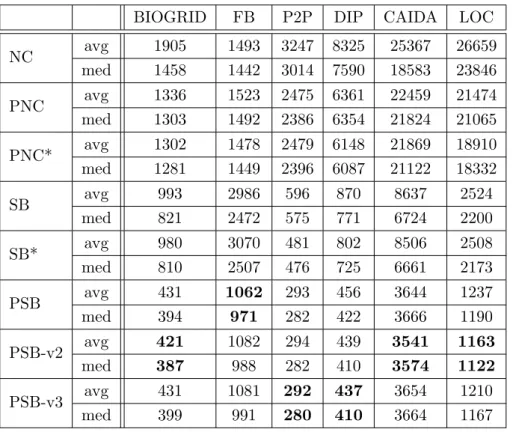
On complex networks, the PSB algorithm is the fastest kSSP algorithm among the
consid-570
ered algorithms (Table 4 and Figure 4). Considering the space consumption, all of the kSSP algorithm have a tiny memory consumption (for k = 10, 000, the number of stored in-branchings does not exceed 50). It is also shown in Table 4 that the running time of PSB and its two variants (PSB-v1 and PSB-v2) is similar.
In what follows, we give some qualitative arguments that may explain the fact that the PSB
575
(a) Running time of SB and SB* (b) Running time of NC and PNC
(c) Running time of SB* and PNC (d) Running time of PNC and PNC*
(e) Running time of SB and PSB (f) Number of trees of SB and PSB
Figure 1: Comparison of the running time and the number of stores trees on DC. Each dot corresponds to one pair source/destination (k = 1, 000).
(a) Running time of SB and SB* (b) Running time of NC and PNC
(c) Running time of SB* and PNC (d) Running time of PNC and PNC*
(e) Running time of PSB and SB (f) Number of trees of SB and PSB
Figure 2: Comparison of the running time and the number of stores trees on COL. Each dot corresponds to one pair source/destination (k = 1, 000).
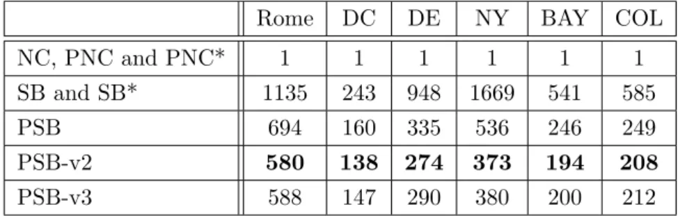
Rome DC DE NY BAY COL Yen avg 3389 11316 159785 - - -med 1439 4945 59463 - - -NC avg 407 823 10620 99521 94149 146025 med 178 404 6129 64465 56136 99540 PNC avg 181 326 1972 41923 24970 35265 med 155 299 1644 39389 24064 35039 PNC* avg 203 336 2434 69913 28481 40045 med 173 305 1997 58446 26552 38952 SB avg 451 184 8469 53423 38390 68077 med 356 75 4321 30300 8783 20535 SB* avg 282 117 5428 33704 28693 49859 med 199 43 2139 18659 4977 11060 PSB avg 447 269 7939 106040 53286 81321 med 340 117 6148 81927 23574 40640 PSB-v2 avg 447 265 7513 100377 49683 76766 med 347 117 5849 75914 21812 38732 PSB-v3 avg 446 265 7471 100390 49653 77185 med 346 115 5785 75681 21770 38709
Table 2: Running time (ms) of the algorithms on road networks, (k = 1, 000)
Rome DC DE NY BAY COL
NC, PNC and PNC* 1 1 1 1 1 1
SB and SB* 1135 243 948 1669 541 585
PSB 694 160 335 536 246 249
PSB-v2 580 138 274 373 194 208
PSB-v3 588 147 290 380 200 212
Table 3: Average number of stored trees using some kSSP algorithms on road networks, (k = 1, 000)
BIOGRID FB P2P DIP CAIDA LOC NC avg 1905 1493 3247 8325 25367 26659 med 1458 1442 3014 7590 18583 23846 PNC avg 1336 1523 2475 6361 22459 21474 med 1303 1492 2386 6354 21824 21065 PNC* avg 1302 1478 2479 6148 21869 18910 med 1281 1449 2396 6087 21122 18332 SB avg 993 2986 596 870 8637 2524 med 821 2472 575 771 6724 2200 SB* avg 980 3070 481 802 8506 2508 med 810 2507 476 725 6661 2173 PSB avg 431 1062 293 456 3644 1237 med 394 971 282 422 3666 1190 PSB-v2 avg 421 1082 294 439 3541 1163 med 387 988 282 410 3574 1122 PSB-v3 avg 431 1081 292 437 3654 1210 med 399 991 280 410 3664 1167
Table 4: Running time (ms) of the algorithms on Complex networks, (k = 10, 000)
(a) Average running time of DC (b) Median running time on DC
(c) Average running time of COL (d) Median running time on COL
Figure 3: The running time of the kSSP algorithms on road network with respect to the values of k
Suppose P is a shortest path from s to t. On complex networks, it is likely to have a vertex v on P with high degree. Let us study the behavior of the different variants of the PSB algorithm when they compute the detours of P at v, in contrast with the other algorithms.
First, Yen’s, NC, PY and PNC algorithms may compute, independently, for each vertex
580
v0 ∈ N+(v) neighbor of v a shortest path from v0 to t resulting with |N+(v)| shortest path
algorithm calls to find the shortest simple detours at the neighbors of v. On the other hand, SB* and PSB algorithms compute at most one shortest path in-branching T at v, that works for each neighbor v0of v. In another word, SB* and PSB are favorable to iterate on v. Moreover, as v has a high degree, it is supposed that a large number of the neighbors v0 of v leads to simple
585
candidates, i.e, PvT0t∩ (s, · · · , v) = ∅. So, the number of shortest path in-branchings computed
and/or stored using SB* and PSB algorithms is expected to be small.
In addition, as the number of hops of a shortest path is “small” (remember that complex network are small-worlds). The number of calls of the shortest path in-branching update is expected to be small for PSB. As this procedure is faster in PSB than SB* and the number of
590
calls is similar, PSB algorithm is faster than SB* on complex networks. This is not valid on road network because the number of hops of a shortest path may be big and the shortest path in-branching update is called many more times.
To conclude, on complex networks, the PSB algorithm is the fastest among the considered algorithms, it has a feasible working memory and this seems to be related to structural properties
595
of complex networks.
(a) Average running time of BIOGRID (b) Median running time on BIOGRID
(c) Average running time of CAIDA (d) Median running time on CAIDA
Figure 4: The running time of the kSSP algorithms on complex network with respect to the values of k
6.3 Impact of the properties of the queries
Here we study the impact of other parameters (related to the properties of the queries) on the running time of the algorithms. In particular, the number of hops of a shortest path and the stretch of a shortest path from the “center” (defined below).
600
As noticed in Section 6.2, some algorithms have different behaviors with respect to the structure of the network and the query’s properties. In this section, we are investigating whether some properties of an s-t query may explain the variations of the running time of the algorithms. For this purpose, we have considered two criteria of each s-t query, the number of hops between s and t of a shortest s-t path and the stretch of a shortest s-t path from the “center” of the
605
graph.
A similar indicator to the number of hops of a shortest path is the maximum number of hops, that is the number of hops of a path with maximum number of hops among the k shortest paths given by an algorithm. Formally, the maximum number of hops of a kSSP query from s to t using an algorithm A is M if and only if for each path P given by A, |P | ≤ M . We studied
610
this parameter and the obtained results are almost the same as those obtained while studying the number of hops. Therefore, we only describe the results corresponding to the number of hops.
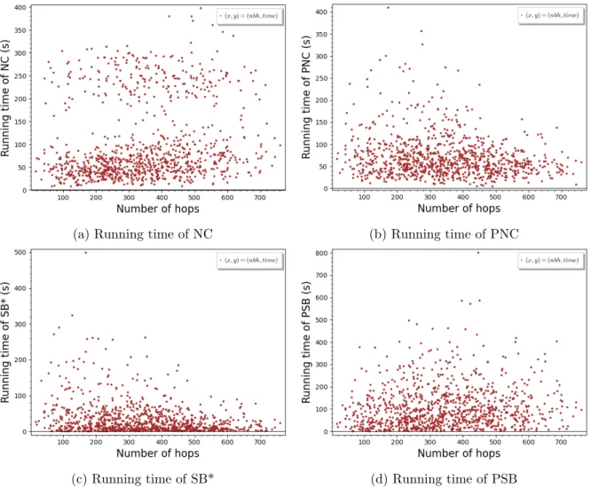
The number of hops of the shortest path (the one given by an SP algorithm) is a meaningful criterion to be studied, as each of the algorithms has the common routine of iterating and
615
eventually calling an SP algorithm for each vertex on the first shortest path. As the obtained results are similar on different road networks, we only add and discuss the results of NC, PNC, SB* and PSB algorithm on NY road network.
As shown in Figure 5, no clear pattern can lead to a establish a concrete relationship between the running time for one of these algorithms and the number of hops. For instance, the SB*
620
algorithms Figure 5c has big running time for queries with relatively small number of hops. However, this is not flagrant and it does not hold on the remaining algorithms (Figures 5a, 5b and 5d).
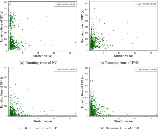
Another interesting parameter to be studied in road networks is the stretch from the center (by center we mean a vertex of minimum eccentricity in the network). So, the stretch of an
625
s-t path P from the center c is defined as the ratio between the length of a shortest s-t path passing through c and the length of P . This gives an indicator on how far a path can be from the center. In order to establish a relation between the running time and the stretch of the center, we plotted (Figure 6) the running time with respect to the stretch value. Clearly, no flagrant pattern related to the stretch value is found. Then, no concrete relation between the
630
running time of these algorithms and the stretch from the center can be established based on our experiments.
To conclude, no clear relationship between the running time of an algorithm and the number of hops, neither the stretch from the center is experimentally found. However, it seems that not all queries perform the same. For instance, in Figures 1b, 2b, 5a and 6a, it can be observed
635
two distinct clouds of points. It would be interesting to understand whether these two clouds correspond to some specific properties of the queries. This could help us to design improvements of our algorithms.
7
Conclusion
In this paper, we have presented several algorithms for the kSSP problem. In particular, we
640
have proposed several new algorithms for this problem with the aim of reducing the running time and / or the working memory consumption of the algorithms.
(a) Running time of NC (b) Running time of PNC
(c) Running time of SB* (d) Running time of PSB
Figure 5: The running time with respect to the number of hops of the shortest path of some kSSP algorithms on NY. Each dot corresponds to one pair source/destination (k = 1, 000).
(a) Running time of NC (b) Running time of PNC
(c) Running time of SB* (d) Running time of PSB
Figure 6: The running time with respect to the stretch from the center of some kSSP algorithms on NY. Each dot corresponds to one pair source/destination (k = 1, 000).
Our simulation results show that the best algorithm to be chosen for solving the kSSP problem depends on the use case. For instance, on the considered complex networks, the PSB algorithm achieves the best results. Indeed, it is the fastest among the considered algorithms,
645
and, similarly to the other algorithms, it has low memory consumption. Besides, on road networks, if large memory consumption is allowed, the SB* algorithm is the fastest among the considered algorithms on most of the queries. However, the PNC algorithm has a running time that is more stable and it has low working memory. Therefore, the PNC algorithm seems to offer a better space time trade-off than the other considered algorithms on road networks.
650
An empirical framework for the selection of the most appropriate kSSP algorithm with respect to the use case is suggested in Figure 7.
An open problem is how to handle the kSSP problem on networks with arbitrarily arc weights (including negative weights). Another interesting question is how to design a data structure enabling to quickly answer kSSP queries similarly to the data structures used by the
655
hub labelling and contraction hierarchy schemes to answer distance queries [3]. A probably more difficult question would be to address dynamic networks, i.e., where the weights of the arcs evolve along time (e.g., in road networks where the traversal time of an arc may vary). Would it be possible to quickly update the solutions after a modification in the network?
kSSP
PSB large
working memory?
SB* PNC
complex network road network
Yes No
Figure 7: A framework of the appropriate kSSP algorithm with respect to the use case
References
660
[1] A. Al Zoobi, D. Coudert, and N. Nisse. k shortest simple paths (Version 2.0), 2021. https://gitlab.inria.fr/dcoudert/k-shortest-simple-paths.
[2] M. Arita. Metabolic reconstruction using shortest paths. Simulation Practice and Theory, 8(1-2):109–125, 2000.
[3] H. Bast, D. Delling, A. Goldberg, M. M¨uller-Hannemann, T. Pajor, P. Sanders, D. Wagner,
665
and R. F. Werneck. Route planning in transportation networks. In Algorithm engineering, pages 19–80. Springer, 2016.
[4] M. Betz and H. Hild. Language models for a spelled letter recognizer. In 1995 International Conference on Acoustics, Speech, and Signal Processing, volume 1, pages 856–859. IEEE, 1995.
670
[5] S. Boccaletti, V. Latora, Y. Moreno, M. Chavez, and D.-U. Hwang. Complex networks: Structure and dynamics. Physics reports, 424(4-5):175–308, 2006.
[6] S. Clarke, A. Krikorian, and J. Rausen. Computing the n best loopless paths in a network. Journal of the Society for Industrial and Applied Mathematics, 11(4):1096–1102, 1963.
[7] C. Demetrescu, A. V. Goldberg, and D. S. Johnson. 9th DIMACS implementation challenge
675
- shortest paths, 2006.
[8] D. Eppstein. Finding the k shortest paths. SIAM Journal on Computing, 28(2):652–673, 1998.
[9] D. Eppstein. Encyclopedia of Algorithms, chapter k-Best Enumeration, pages 1003–1006. Springer New York, 2016.
680
[10] D. Eppstein and D. Kurz. K-best solutions of MSO problems on tree-decomposable graphs. In 12th International Symposium on Parameterized and Exact Computation (IPEC 2017), volume 89, pages 16:1–16:13. Schloss Dagstuhl - Leibniz-Zentrum f¨ur Informatik, 2017.
[11] G. Feng. Finding k shortest simple paths in directed graphs: A node classification algo-rithm. Networks, 64(1):6–17, 2014.
685
[12] M. L. Fredman, R. Sedgewick, D. D. Sleator, and R. E. Tarjan. The pairing heap: A new form of self-adjusting heap. Algorithmica, 1(1):111–129, 1986.
[13] D. Frigioni, A. Marchetti-Spaccamela, and U. Nanni. Fully dynamic algorithms for main-taining shortest paths trees. Journal of Algorithms, 34(2):251–281, 2000.
[14] J. Gao, H. Qiu, X. Jiang, T. Wang, and D. Yang. Fast top-k simple shortest paths discovery
690
in graphs. In Proceedings of the 19th ACM international conference on Information and knowledge management, pages 509–518, 2010.
[15] Z. Gotthilf and M. Lewenstein. Improved algorithms for the k simple shortest paths and the replacement paths problems. Information Processing Letters, 109(7):352–355, 2009.
[16] E. Hadjiconstantinou and N. Christofides. An efficient implementation of an algorithm for
695
finding k shortest simple paths. Networks, 34(2):88–101, 1999.
[17] Y. Han and T. Takaoka. An O(n3log log n/ log2n) time algorithm for all pairs shortest paths. Journal of Discrete Algorithms, 38:9–19, 2016.
[18] J. Hershberger, M. Maxel, and S. Suri. Finding the k shortest simple paths: A new algorithm and its implementation. ACM Transactions on Algorithms, 3(4):45, 2007.
700
[19] W. Jin, S. Chen, and H. Jiang. Finding the k shortest paths in a time-schedule network with constraints on arcs. Computers & operations research, 40(12):2975–2982, 2013.
[20] D. S. Johnson. A theoretician’s guide to the experimental analysis of algorithms. Data structures, near neighbor searches, and methodology: fifth and sixth DIMACS implementa-tion challenges, 59:215–250, 2002.
705
[21] N. Katoh, T. Ibaraki, and H. Mine. An efficient algorithm for k shortest simple paths. Networks, 12(4):411–427, 1982.
[22] D. Kurz. k-best enumeration - theory and application. Theses, Technischen Universit¨at Dortmund, Mar. 2018.