HAL Id: halshs-00336475
https://halshs.archives-ouvertes.fr/halshs-00336475
Submitted on 4 Nov 2008HAL is a multi-disciplinary open access archive for the deposit and dissemination of
sci-L’archive ouverte pluridisciplinaire HAL, est destinée au dépôt et à la diffusion de documents
Efficient Frontier for Robust Higher-order Moment
Portfolio Selection
Emmanuel Jurczenko, Bertrand Maillet, Paul Merlin
To cite this version:
Emmanuel Jurczenko, Bertrand Maillet, Paul Merlin. Efficient Frontier for Robust Higher-order Moment Portfolio Selection. 2008. �halshs-00336475�
Documents de Travail du
Centre d’Economie de la Sorbonne
Maison des Sciences Économiques, 106-112 boulevard de L'Hôpital, 75647 Paris Cedex 13
Efficient Frontier for Robust Higher-order Moment Portfolio Selection
Emmanuel F. JURCZENKO, Bertrand B. MAILLET, Paul M. MERLIN
Efficient Frontier for Robust
Higher-order Moment Portfolio Selection
∗
Emmanuel F. Jurczenko† Bertrand B. Maillet‡ Paul M. Merlin§
October 2008
Abstract
This article proposes a non-parametric portfolio selection criterion for the static asset allocation problem in a robust higher-moment framework. Adopting the Short-age Function approach, we generalize the multi-objective optimization technique in a four-dimensional space using L-moments, and focus on various illustrations of a four-dimensional set of the first four L-moment primal efficient portfolios. Our em-pirical findings, using a large European stock database, mainly rediscover the earlier works by Jean (1973) and Ingersoll (1975), regarding the shape of the extended higher-order moment efficient frontier, and confirm the seminal prediction by Levy and Markowitz (1979) about the accuracy of the mean-variance criterion.
∗W e a re g ra te fu l to C h ris to p h e B o u ch e r, T h ie rry C h a u ve a u , J e a n -P h ilip p e M é d e c in , T h ie rry M ich e l a n d P a trick R o g e r fo r h e lp a n d
e n c o u ra g e m e nt in p re p a rin g th is w o rk . W e a ck n ow le d g e P a trick K o u o ntch o u a n d G h is la in Ya n o u fo r e x c e lle nt p re lim in a ry re se a rch a ss ista n c e a n d a n a c tive p a rtic ip a tio n in e a rlie r ve rsio n s . W e a ls o th a n k N a th a lie P ic a rd , P ie rre -C h a rle s P ra d ie r a n d D id ie r R u lliè re fo r p rov id in g u s w ith inte re stin g c o m p le m e nta ry re fe re n c e s. T h e se c o n d a u th o r th a n k s th e E u ro p la c e In stitu te o f F in a n c e fo r fi n a n c ia l su p p o rt. T h e u su a l d is c la im e rs a p p ly.
†E S C P -E A P.
Efficient Frontier for Robust
Higher-order Moment Portfolio Selection
Abstract
This article proposes a non-parametric portfolio selection criterion for the static asset allocation problem in a robust higher-moment framework. Adopting the Short-age Function approach, we generalize the multi-objective optimization technique in a four-dimensional space using L-moments, and focus on various illustrations of a four-dimensional set of the first four L-moment primal efficient portfolios. Our em-pirical findings, using a large European stock database, mainly rediscover the earlier works by Jean (1973) and Ingersoll (1975), regarding the shape of the extended higher-order moment efficient frontier, and confirm the seminal prediction by Levy and Markowitz (1979) about the accuracy of the mean-variance criterion.
Since the first mention of higher-order moments than the variance of returns by Marschak (1938) and Hicks (1939), it is now generally accepted by the financial community that in-vestors generally exhibit preferences for positively skewed and light-tailed asset return distributions (see, for instance, Beedles and Simkowitz (1978), Dittmar (2002), Jurczenko and Maillet (2006a), and Mitton and Vorkink (2007)). Developments with higher moments followed since the origin three main (complementary) directions in finance: a tentative in-tegration in the von Neumann-Morgenstern utility function of a rational investor (Cf. Arrow (1964) and Pratt (1964)) of higher-order moments of returns by Arditti (1967), Samuelson (1970) and Tsiang (1972); an attempt to generalize the Markowitz (1952) ef-ficient frontier to incorporate the effect of higher moments on optimal asset allocations by Jean (1971 and 1973), Arditti and Levy (1972), Ingersoll (1975) and Schweser (1978); and a first partial explicit modelling of returns by Rubinstein (1973), and Kraus and Litzenberger (1976), through extensions of the CAPM by Sharpe (1964). True departures
from Gaussianity may indeed affect the optimal allocation of assets (see Jondeau and Rockinger (2003b and 2006a)) and the mean-variance portfolio selection criterion pro-posed by Markowitz (1952) is a priori somehow inadequate for some risky assets whose characteristics are very special (see Jondeau and Rockinger (2006a)). In such a context, different multi-moment approaches have been proposed in the financial literature to in-corporate higher-order moment preferences into asset allocation problems1, in order to
characterize generalized geometric efficient frontiers (see Athayde and Flôres (2002 and 2003)); but all suffer more or less from the traditional drawbacks of algebraic moments. First, higher-order moments do not always exist (see Embrechts, Kluepelberg and Mikosh (1997), and Jondeau and Rockinger (2003a and 2003b)), and even when they do, such moments do not always uniquely define a probability distribution, so that two distinct distributions can have the same sequence of moments (see Heyde (1963) for the example of the Log-normal density). Secondly, conventional moments tend to be very sensitive to a few extreme observations (see Hampel, Ronchetti, Rousseeuw and Stahel (2005)). The asymptotic efficiency of the empirical moments is also rather poor, especially for distrib-utions with fat tails. This last property is an immediate consequence of the fact that the asymptotic variances of these estimators are mainly determined by higher-order moments, which tend to be rather large, or even unbounded, for heavy-tailed distributions.
The objective of this paper is to overcome the limits of traditional multi-moment as-set allocation models by using an alternative as-set of statistics in traditional optimization programs, namely L-moments. Recent attempts for modelling distributions in a multi-variate framework are indeed built on the concept of order-statistics, for calibrating a Bernstein Copula in Baker (2008) or for defining extreme co-movements using L-moments in Serfling and Xiao (2007). The latter, which are linear functions of the expectations of order statistics, were introduced under this name by Sillitto (1951) and comprehensively reviewed by Hosking (1989). As so-called U-statistics (see Hoeffding (1948)), L-moments offer one main advantage over Conventional moments (denoted herein C-moments as in Ulrych, Velis, Woodbury and Sacchi (2000), and Chu and Salmon (2008)). Their empirical counterparts are less sensitive to the effects of sampling variability, since they are linear functions of the ordered data, and are therefore shown to provide more robust estimators
1See Athayde and Flôres (2002 and 2006), Briec, Kerstens and Jokung (2007), Jurczenko and
Mail-let (2006b), and Jurczenko, MailMail-let and Merlin (2006) for the primal approaches of the mean-variance-skewness-kurtosis portfolio decision problems; and Simaan (1993), Gamba and Rossi (1998a and 1998b), Jurczenko and Maillet (2001 and 2006a), and Jondeau and Rockinger (2006a) for the dual approaches of
of higher moments than the corresponding sample C-moments (Sankarasubramanian and Srinivasan (1999)). More precisely, L-moments are defined as certain linear functions of the Probability Weighted Moments (Greenwood, Landwehr, Matalas and Wallis (1979)) and can characterize a wider range of distributions compared to C-moments. Indeed, they exist whenever the mean of the distribution does, even though some C-moments do not (which is very likely to be the case in finance). As we will see later on, they are also particularly well adapted for addressing some specific concerns in the field of finance. And the beauty is that they are easy and fast(er) to compute, besides being reliable estimators of characteristic shape parameters of general distributions.
Because of their proven advantages, L-moments have already found wide applications in various fields such as meteorology, hydrology, geophysics and regional analysis (see Hosking and Wallis (1997)) - where large deviations really matter, namely for instance when studying extreme floods or low flows (see among the main references: Hosking and Wallis (1987), Ben-Zvi and Azmon (1997), Wang (1997), Bayazit and Önöz (2002), Moi-sello (2007), and Shao, Chen and Zhang (2008)), rainfall extremes (see Guttman, Hosking and Wallis (1993), Lee and Maeng (2003), and Parida and Moalafhi (2008)), raindrop sizes (see Kliche, Smith and Johnson (2008)), velocity of gale force winds (see Pandey, Gelder and Vrijling (2001), Whalen, Savage and Jeong (2004), and Modarres (2008)) or the measurement of earthquake intensities (Thompson, Baise and Vogel (2007)). Lately, they have also found an interest in finance, first, as Monsieur Jourdain by Molière with-out noticing it, when using a special case of an L-moment which is the Gini coefficient (see Gini (1912) and below) as a substitute to the volatility in asset pricing models (see Shalit and Yitzhaki (1989), Okunev (1990), and Benson, Faff and Pope (2003)); then, secondly, for more general purposes: for fitting return distributions (Hosking, Bonti and Siegel (2000), Carrillo, Hernández and Seco (2006a), and Karvanen (2006)) and the rate of profit densities (Wells (2007)), the design of a GMM-type Goodness-of-Fit test (see Chu and Salmon (2008)), risk modelling purposes (see Martins-Filho and Yao (2006), Tolikas and Brown (2006), Tolikas, Koulakiotis and Brown (2007), Gouriéroux and Jasiak (2008), and Tolikas (2008)), calibrating extreme return distributions (Gettinby, Sinclair, Power and Brown (2006), French (2008), and Tolikas and Gettinby (2008)) or rogue-volatility densities (Maillet and Médecin (2008), and Maillet Médecin and Michel (2008)), and very recently for defining a new set of measures of performance for hedge funds (see Darolles, Gouriéroux and Jasiak (2008)).
Thanks to the so-called shortage function technique and relying on robust L-statistics, we thus generalize in this article the traditional mean-variance-skewness-kurtosis efficient
frontier in the four L-moment space, proposing a new and fast formulation of higher-order (L-)comoments of efficient portfolios. The shortage function of Luenberger (1995) was in-deed first applied to the portfolio performance evaluation in the traditional mean-variance framework by Morey and Morey (1999), then developed by Briec, Kerstens and Lesourd (2004), and recently extended to multi-horizon performance appraisals (Briec and Ker-stens (2009)). In brief, the shortage function rates the performance of any portfolio by measuring a distance between the coordinates of this specific portfolio and those of its ra-dial projection onto the multi-moment efficient frontier. Based on this distance definition, the so-called Goal Attainment Method enables us to solve the multiple conflicting and competing allocation objectives, without assuming a detailed knowledge of the preference parameters of the indirect investor’s utility function.
After a theoretical presentation of L-moments and of the shortage function approach in a portfolio selection context, we propose to rewrite the multi-moment optimization program of the investor within a new compact notation, using both C-moments and L-moments, then derive the four L-moment efficient set and provide various illustrations using a universe of 162 European stocks. Our empirical results regarding links between moments of efficient portfolios and the various shapes of the higher-order moment efficient frontier - from (pseudo-)parabolae to (deformed) cones, confirm the earlier findings by Jean (1973) and Ingersoll (1975) presenting the first three-dimensional representation of the efficient set. They are also consistent with more recent evidences provided in other frameworks (see for instance, Athayde and Flôres (2004), Jurczenko, Maillet and Merlin (2006), Maringer and Parpas (2008)). However, it is worth noting that our attempt to evaluate the cost of not using higher-order moments is still not conclusive in a traditional “mixed” utility setting, since differences between optimal asset allocation implied utilities are found to be marginal. In other words, the mean-variance criterion - corner stone of the Modern Portfolio Theory of de Finetti2 (1940) and Markowitz (1952) - is shown to
be rather accurate as predicted, among others, by Levy and Markowitz (1979) and Kroll, Levy and Markowitz (1984). As mentioned by Jondeau and Rockinger (2006a), the use of higher-order moments, in a the traditional expected utility framework and in a restrictive “mixed” utility setting (in which sensitivities only depends upon the first moment), may thus only prove their efficiency either if the underlying assets are largely non-Gaussian (in some specific sense) or if the representative investor exhibits some very peculiar features regarding her prudence and temperance characteristics. Nevertheless, we also suggest that
complementary controls of higher-order moments of some traditional low-dispersion return efficient portfolios (such as the Global Minimum-Variance Portfolio) may be of interest for the investors.
The remainder of the article is organized as follows. In section 2, we formally present the L-moments, briefly recall some of their main properties, and illustrate their compu-tations on a long record of stock index quotes. In section 3, we precisely define in a new notation higher-order moments of returns on portfolios and describe how the optimal portfolio selection L-moment program can be solved in a shortage function framework. In section 4, we present the data and discuss the results of the various optimal asset al-locations. Section 5 concludes. The Appendices are dedicated to proofs, some technical details, Tables and Figures.
I.
Robust Higher-order Moments for Portfolio
Selec-tion
Introduced by Sillitto (1951) and popularized by Hosking (1989), L-moments can be inter-preted, like C-moments, as simple descriptors of the shape of a general distribution, albeit offering a number of advantages.
First, all population (higher) L-moments exist and uniquely determine a probability distribution, provided that the mean exists (see Chan (1967), and Arnold and Meelden (1975)). In this case, a distribution can always be specified by its L-moments, even if some of its higher-order C-moments do not exist. Furthermore, this specification is always unique. For the standard errors of L-moments to be finite, it is also only required that the distribution has a finite variance; no condition on higher-order moments is necessary (Hosking (1990)). Moreover, although moment ratios can be arbitrarily large, sample mo-ment ratios have algebraic bounds (see Dalén (1987)) and sample L-momo-ment ratios can take any values that the corresponding population quantities can (Hosking (1990)). Moti-vated by the sampling properties of L-statistics, Hosking and Wallis (1987) thus advocate that L-moments provide a better approximation of the unknown parent distribution than C-moments. They also provide reliable estimators for Extreme Value densities and have been widely used in fields where exceptions are at stake (see Hosking (1990)).
Secondly, L-moments exhibit some specifically interesting features for financial applica-tions. Since a (complete) set of L-moments determine a unique density, the so-called Ham-burger problem (see Jondeau and Rockinger (2003a) and Jurczenko and Maillet (2006a))
- when C-moments lead to several laws - is limited. Since they always exist, the problem of working with non-defined quantities such as higher C-moments is avoided. L-moments are also coherent shape measures of risk (see Artzner, Delbaen, Eber and Heath (1999)), since they are translation and scale invariants (Serfling and Xiao (2007), and Gouriéroux and Jasiak (2008)). They, furthermore, allow us a clearer focus on a specific part of the distribution, thus avoiding confusion between the center and the extreme parts of the distribution as in the traditional case (see Haas (2007)). Finally, the sample estimates of L-moments are more robust to data outliers (Vogel and Fennessey (1993)) - since they are only linearly influenced by large deviations (see Hosking (1990)) - and more efficient than C-moments (see Sankarasubramanian and Srinivasan (1999), and Carrillo, Hernández and Seco (2006b)), especially within a Generalized Method of (L-)Moment context (see Get-tinby, Sinclair, Power and Brown (2006), Chu and Salmon (2008), and also Gouriéroux and Jasiak (2008)).
After having briefly recalled the different analytical representations of the univariate population L-moments3 - we mainly refer here to the work by Hosking and Wallis (1997),
we will present in the following sub-section their sample unbiased estimator counterparts and shall illustrate the four first L-moment estimates on a long sample of one century of daily quotes of the Dow Jones Index.
A.
Population L-comoments
Population L-moments are defined as certain linear functions of the expectations of the order statistics from the population distribution of the underlying random variable. Let us start with some basic notations and definitions.
Let {Xt}, with t = [1, ..., T ], be a conceptual random sample of size T drawn from
a continuous probability distribution F (.) of a real-valued random variable X, with T ∈ IN∗; Q (u) = F−1(u) , for u =]0, 1[, a quantile function, and X
[1:T ] ≤ X[2:T ] ≤ ... ≤
X[T :T ] denoting the corresponding order statistics. Then the k-th population univariate
L-moment (using the L-functional representation) is defined, ∀k ∈ IN∗ and k < T , as
3Other variants of L-moments, called TL-moments (encompassing the PL-moments, the LH-moments
and the LL-moments), LQ-moments (see Maillet and Médecin (2008), for a comprehensive review and an application to extreme volatilities), as well as the LSD-moments (SD-PWM - see Haktanir (1997), and Whalen, Savage and Jeong (2004)), have already been used in extreme studies, since they are proven to be even less sensitive to outliers. However, to be as close as possible to the portfolio value as perceived by the investors, we will stick, in this article, with the traditional simple L-moments in our portfolio context.
(see, for instance, Hosking (1990)): λk(X) = k−1P j=0 (−1)j©[k (k− j − 1)!j!]−1[(k− 1)!]ª× E¡X[k−j:k]¢ = R01Q (u) P∗ k−1(u) du, (1) with: ⎧ ⎪ ⎪ ⎪ ⎨ ⎪ ⎪ ⎪ ⎩ E¡X[r:k] ¢ = ©[(r− 1)! (k − r)!]−1(k!)ª×R01Q (u) ur−1(1− u)k−rdu P∗ k (u) = k P r=0 p∗ k, rur p∗ k, r = (−1)k−r n£ (r!)2(k− r)!¤−1(k + r)!o,
where λk(.)is the L-moment of order k, r = [1, ..., k], 0 < u < 1, E (.) is the expectation
operator and p∗k, r corresponds to the r-th coefficient of the shifted orthogonal Legendre polynomial of degree k denoted Pk∗(.) and defined as Pk∗(u) = Pk(2u− 1) where Pk(.) is
the traditional Legendre polynomial of degree k.
Thus, the shifted orthogonal Legendre polynomial satisfies, ∀ (k, s) ∈ IN∗2: ( R1 0 Pr∗(u) Ps∗(u) du = (2r− 1)−1 = 0 if r = s if r 6= s, (2) with P∗ 0 (u) = 1.
In particular, the first four population L-moments are: ⎧ ⎪ ⎪ ⎪ ⎨ ⎪ ⎪ ⎪ ⎩ λ1(X) = E ¡ X[1:1] ¢ λ2(X) = (2)−1E ¡ X[2:2]− X[1:2] ¢ λ3(X) = (3)−1E £¡ X[3:3]− X[2:3] ¢ −¡X[2:3] − X[1:3] ¢¤ λ4(X) = (4)−1E £¡ X[4:4]− X[1:4] ¢ − 3¡X[3:4]− X[2:4] ¢¤ . (3)
Knowing relation (1), they also satisfy the following equalities: ⎧ ⎪ ⎪ ⎪ ⎨ ⎪ ⎪ ⎪ ⎩ λ1(X) = R1 0 Q (u) du λ2(X) = R1 0 Q (u) (2u− 1) du λ3(X) = R1 0 Q (u) (6u 2 − 6u + 1) du λ4(X) = R1 0 Q (u) (20u 3 − 30u2+ 12u − 1) du. (4)
Note that λ1(.) , λ2(.) , λ3(.) and λ4(.) are population measures of location, scale and
shape, strictly analogous to the corresponding traditional central moments. The first L-moment is the mean of the population distribution and the second L-L-moment, defined
in terms of a conceptual random sample of size 2, is a measure of the typical spread of the random variable X, being half the expected value of Gini’s Mean Difference (see Gini (1912)), which has some desirable properties in finance when replacing the traditional vari-ability measure (see Yitzhaki (2003)). In short, the third L-moment simply represents the difference between the upper tail and the lower tail, and hence measures the asymmetric shape of the population distribution from which the conceptual random sample has been drawn. Similarly, the fourth L-moment measures the kurtosis of the probability distribu-tion funcdistribu-tion, and can be expressed as a (rescaled) difference between the typical spread in the tails and the typical spread in the center.
While Equation (1) is the classical L-functional’s representation for the population L-moments, there exist several other representations for λk(.) that prove to be useful
for financial applications (see below). For example, using the definition of the Probability Weighted Moments, we can also express Equation (1) as a linear function of the Probability Weighted Moments, that is (see Hosking (1989)):
λk(X) = k X r=1 p∗k−1, r−1βr−1(X) , (5) with: βr−1(X) = r−1E¡X[r:r] ¢ = Z 1 0 Q (u) ur−1du,
where k ∈ IN∗, βr(.) are the Probability Weighted Moments of order r, with r =
[2, ..., k], and p∗k−1, r−1 is the (r − 1)-th coefficient of the shifted Legendre polynomial of degree (k − 1) defined in Equation (1).
Using the definition and orthogonal property of the shifted Legendre polynomials, the k-th population L-moment can also be represented as the covariance between the random variable X and its distribution function denoted F (.), that is (see Serfling and Xiao (2007)): λk(X) = ( E (X) Cov©X, Pk−1∗ [F (X)]ª if k = 1 if k 6= 1, (6) with: E{Pk∗[F (X)]} = Z 1 0 Pk∗(u) du = 0,
Since E [F (X)] = 1/2, relation (6) allows us to obtain alternative expressions for the first four population L-moments such as:
⎧ ⎪ ⎪ ⎪ ⎨ ⎪ ⎪ ⎪ ⎩ λ1(X) = E (X) λ2(X) = 2 E{[X − E (X)] × [F (X) − E [F (X)]]} λ3(X) = 6E © [X− E (X)] × [F (X) − E [F (X)]]2ª λ4(X) = 20E © [X− E (X)] × [F (X) − E [F (X)]]3ª− 3 (2)−1λ2(X) , (7)
where λ1(.) and λ2(.) represent respectively the (L-)mean and the L-variance, and λ3(.)
and λ4(.) correspond to the unscaled L-skewness and L-kurtosis of the population
distri-bution F (.).
The population L-moments presented in Equation (7) are defined for a given probability distribution, but, in practice, they are directly estimated with some uncertainty from a finite sample draw, corresponding to an unknown distribution. The following sub-section is devoted to a brief presentation of the (original) sample counterparts of the population L-moments.
B.
Sample Portfolio Return L-moments
Following Hosking (1989), sample L-moments can be estimated in a straightforward man-ner by estimating the empirical Probability Weighted Moments, denoted ˆβr(.), in
con-junction with their L-statistic representations in (5).
Indeed, let X[1:T ] ≤ X[2:T ] ≤ ... ≤ X[T :T ] be again the order statistics of a random
sample {Xt} of size T , drawn from a continuous non-degenerated probability distribution
F (.) of a real-valued random variable X, with t = [1, ..., T ] and T ∈ IN∗. The r-th
Probability Weighted Moment estimator is given, ∀r ∈ IN∗ and 1 < r < T , by:
bβr(X) = (T )−1× T X t=1 ( r Y j=1 ∙ (t− j) (T − j) ¸ X[t:T ] ) , (8)
where bβr(.)is the unbiased estimator of βr(.) .
Thus, for a sample of size T , the k-th sample L-moment is defined as: bλk(X) =
k
X
r=1
p∗k−1, r−1βbr−1(X) , (9)
where bλk(X) is the k-th sample L-moment corresponding to the population L-moment
λk(.) of a real-valued random variable X, (r × k × T ) ∈ (IN∗) 3
is the (r − 1)-th coefficient of the shifted Legendre polynomial of degree (k − 1) defined as in Equation (1).
The L-moment estimator (9) is an unbiased L-statistic estimator of the population L-moment. In particular, in a time-series context, the first four sample L-moments from (9) are given by (with previous notations):
⎧ ⎪ ⎪ ⎪ ⎪ ⎪ ⎪ ⎪ ⎪ ⎪ ⎪ ⎪ ⎪ ⎪ ⎪ ⎪ ⎪ ⎪ ⎨ ⎪ ⎪ ⎪ ⎪ ⎪ ⎪ ⎪ ⎪ ⎪ ⎪ ⎪ ⎪ ⎪ ⎪ ⎪ ⎪ ⎪ ⎩ bλ1(X) = (T )−1 T P t=1 X[t:T ] bλ2(X) = [T (T − 1)]−1 T P t=1 (2t− 1 − T ) X[t:T ] bλ3(X) = [T (T − 1) (T − 2)]−1 T P t=1 [6 (t− 1) t − 6 (t − 1) T + (T − 1) (T − 2)] X[t:T ] bλ4(X) = [T (T − 1) (T − 2) (T − 3)]−1 × T P t=1 [20 (t− 1) (t − 2) (t − 3) − 30 (t − 1) (t − 2) (T − 3) +12 (t− 1) (T − 2) (T − 3) − (T − 1) (T − 2) (T − 3)] X[t:T ]. (10)
Under the second central moment existence condition, the standard theory for U-statistics and L-U-statistics states that the (first) k-th sample L-moments are asymptotically jointly normally distributed, with a similar result for the vector of the sample L-moment ratios (see, for instance, Hoeffding (1948)).
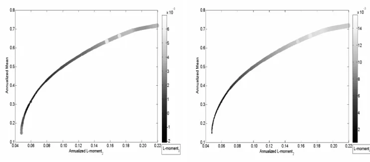
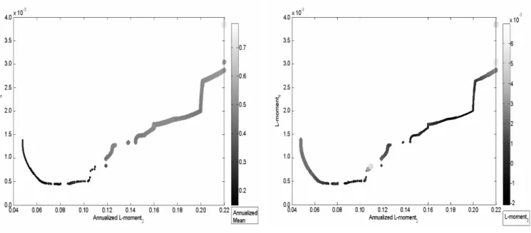
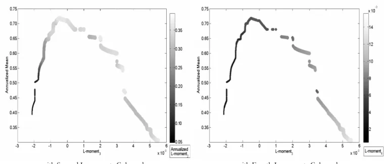
Figure 1 illustrates the first (rescaled) L-moment estimations against the traditional sample moments, calculated on a long sample of one century of daily quotes of the Dow Jones Index. The set of figures on the left part (Figure 1) corresponds to time-evolutions of the second, third and fourth moments, recursively computed since the 1st of January
1900, whilst the set of right figures represents the one-year rolling window first moment non-parametric empirical densities. As expected, it is clear from these figures that sam-ple L-moments are far more stable than C-moment estimates. Moreover, densities of L-moments are more concentrated around a unique mode of L-moment values and exhibit fewer extreme values, indicating faster decreasing tails. This visually confirms that higher-order L-moments are less prone to the influence of outliers, and thus may be seen as more accurate.
Please, Insert Figure 1 somewhere here
quanti-by using the shortage function approach of Luenberger (1995), the mean-variance efficient frontier in the first four L-moment space.
II.
Portfolio Selection with Higher-order Moments
In the context of portfolio selection, the aim of the investors is to determine their asset allocation in order to maximize their utility function. We refer here to a general class of utility functions exhibiting a “mixed” risk aversion respecting the fourth-order stochastic dominance criterion (see Caballé and Pomansky (1996)), which alternate the signs of par-tial derivatives. In such a setting, we thus consider an exact (or accurate approximative) fourth-order Taylor expansion of a general utility function (see for details Jurzcenko and Maillet (2006a), and Garlappi and Skoulakis (2008)) with a strictly (monotone) increas-ing first derivative representative of the preference of non-satiable individuals, a strictly decreasing second derivative for risk-averse agents, a strictly increasing third derivative for prudent investors, and a strictly decreasing fourth derivative for temperate behaviors. More precisely (see Appendix 1 for a few illustrations with some usual utility functions), the expected utility of the random return on a portfolio p (denoted Rp) held by a rational
investor, can be represented by an indirect utility function, denoted V (.), successively, concave and increasing with the expected return - denoted E (Rp), concave and decreasing
with the variance - reading σ2(R
p), concave and increasing with the skewness - written
m3(R
p), and, concave and decreasing with the kurtosis4 - defined by κ4(Rp). Such an
expected utility function can be written in a general form as: E [U (Rp)] = V £ E (Rp) , σ2(Rp) , m3(Rp) , κ4(Rp) ¤ , (11) with: V1 = ∂ E(R∂ V (.) p) > 0, V2 = ∂ V (.) ∂ σ2(R p) < 0, V3 = ∂ V (.) ∂ m3(R p) > 0 and V4 = ∂ V (.) ∂ κ4(R p) < 0,
where Rp = W/W0− 1 is the (random) return on the portfolio p held by the investors,
with W0 their initial wealth (being equal to unity for the sake of simplicity), W their
ran-dom final wealth, and V (.) a general (non-)linear indirect utility function whose arguments are the first four conventional moments of returns on portfolio p.
4Whilst, in general, skewness and kurtosis correspond to the standardised third and fourth centered
The various first derivatives of such a general indirect utility function characterize at the same time both economic agent behavioural assumptions - his rational reaction to increases in downside risk, fear of ruin, will of self-protection and self-insurance (see Chiu (2005 and 2008), Crainich and Eeckhoudt (2008)), and a (simple) transformation of a density function of his return on wealth (see, for instance, Eeckhoudt, Gollier and Schneider (1995)). More precisely, the first derivative with respect to the expected return governs the so-called “greediness” of the investor, the second sensitivity represents his “risk aversion”, whilst the third5 and fourth terms characterize respectively the “prudence” (Kimball (1990) and
Lajeri-Chaherli (2004)) and “temperance” (Kimball (1992 and 1993), Eeckhoudt, Gollier and Schneider (1995), Menezes and Wang (2005))6.
From a theoretical point of view, the link between moments and preferences (Scott and Horwath (1980)) is still under question for at least four main reasons. First, moments are only single statistics that can only be imperfect summaries of the plain return distribution characteristics (see Romano and Siegel (1986))7. Depending on the exact transfer
(pre-serving function) of probability weights, we can imagine all sorts of density distortions that basically break the rationale of the investor choice when comparing asset allocations (see Brockett and Kahane (1992) for some explicit examples). Secondly, first moments merely share the same information contained in the return series: the higher the order (and the power of the conventional moment), the more important the focus on the tail and extreme events ceteris paribus. Hence, some of them exhibit certain correlations per construction. In other words, redundant information8 is present in the various comoments (see
Galaged-5Some interesting recent works, however, also show that the ratio [U000(.) /U0(.)] is also link to a risk
aversion characteristic of a rational agent, who makes an arbitrage between the first and the third moments (Cf. Crainich and Eeckhoudt (2008)).
6Lajeri-Chaherli (2004) extends the expansion to the order five, mentioning in reference the fifth-order
risk apportionment “edginess”, whilst Caballé and Pomansky (1996) refine even further the expansion to the n-th order, referring to the “risk aversion of order n”, as an analogue to the traditional classical absolute risk aversion (see also Eeckhoudt and Schlesinger, (2006)). However, to our knowledge, no more precise label of utility characteristic yet exists for extensions to higher-order moments than the fifth. In the following, we nevertheless restrict our analysis to the four first moments, mainly for the sake of tractability, but also due to some questions regarding the existence of empirical counterparts of higher-order C-moments.
7The counterexample they mentioned being that the apparently left-skewed distribution of x =
{−2, 1, 3} with associated probabilities of f(x) = {.4, .5, .1}, has a null skewness.
8It is straightforward to show, for instance, that some terms in the conventional cokurtosis matrix also
era and Maharaj (2008)). Thirdly, the explicit expressions of links between moments and preferences strongly depend upon the precise preference definition (see Haas (2007)) and on the performance of measures of higher-order moments (see Kim and White (2004), for various measures). Fourthly, in a more general prospect theory framework (Kahneman and Tversky (1979)), the rational investor may also further relax the linearity-in-probability property inherent in expected utility theory, by allowing the physical probabilities to be nonlinearly subjectively transformed into “decision weights” (see Kliger and Levy (2008)). Nevertheless, from a more practical point of view, a wealth of literature (see Jondeau and Rockinger (2006a), Jurczenko and Maillet (2006a), and Briec and Kerstens (2007), for a precise reference list on the subject) points out a realistic positive preference of investors for the highest right asymmetries and the lowest tail-fatnesses; we will take this common sense hypothesis as granted in the following, where we simply try to extend the two-moment Markowitz’ analysis in an expected utility framework, only considering higher moments with better properties.
Since we will also only consider “mixed” utility functions, the signs of the sensitivities Vn (partial derivatives), for n = [1, ..., 4], will alternate. Furthermore, in a portfolio
con-text, one could intuitively expect that the investor cares more about a (positive) expected return than about other characteristics9, and, as a result, that the sensitivities decrease
with the order of related moments.
In such a framework, the agent’s portfolio general problem can be stated as (with previous notations): Max w0p {E [U (Rp)]} = Max w0p {V [E (Rp) , σ2(Rp) , m3(Rp) , κ4(Rp)]} s.t. : wp01N =1, (12) where 1N is the (N × 1) unit vector and V (.) a general non-explicited (non-)linear function
depending on the four first C-moments of returns on portfolio p that we explicit hereafter.
9It is difficult to believe that most rational investors care more about higher-order moments than
about the expected return in their asset allocation decisions (which can be the case in a lottery for instance, where the potential big prize may entail a large skewness, allowing them to forget in some sense the likely negative profit of the game). This is the reason why in the following, we further restrict the search for optimal portfolios in regions where the expected returns are positive, and only select, in some representations, portfolios where impacts on the utility functions of moments are ranked according to their order (see Section 4).
A.
Higher-order C-comoments of Portfolio Returns
Actually, the mean, variance, skewness and kurtosis of portfolio p returns used in Equation (11) are given by, with (i, j, k, l) = [1, ..., N ]4 (and with previous notations):
⎧ ⎪ ⎪ ⎪ ⎪ ⎪ ⎪ ⎪ ⎪ ⎪ ⎪ ⎪ ⎨ ⎪ ⎪ ⎪ ⎪ ⎪ ⎪ ⎪ ⎪ ⎪ ⎪ ⎪ ⎩ E (Rp) = N P i=1 wpiE (Ri) σ2(R p) = E © [Rp− E (Rp)]2 ª = N P i=1 N P j=1 wpiwpjσij m3(Rp) = E © [Rp− E (Rp)]3 ª = N P i=1 N P j=1 N P k=1 wpiwpjwpkmijk κ4(R p) = E © [Rp − E (Rp)]4 ª = N P i=1 N P j=1 N P k=1 N P l=1 wpiwpjwpkwplκijkl, (13) with: ⎧ ⎪ ⎨ ⎪ ⎩ σij = E{[Ri− E (Ri)] [Rj− E (Rj)]} mijk= E{[Ri− E (Ri)] [Rj − E (Rj)] [Rk− E (Rk)]} κijkl = E{[Ri− E (Ri)] [Rj − E (Rj)] [Rk− E (Rk)] [Rl− E (Rl)]} ,
where wpi, Ri, σij, mijk and κijkl represent, respectively, the weight of the asset i in
portfolio p, the return on the asset i, the covariance between the returns on assets i and j, the coskewness between the returns on assets i, j and k, and the cokurtosis between the returns on assets i, j, k and l.
These various C-moments of portfolio returns were previously written in a matrix format (see Diacogiannis (1994), Athayde and Florès (2002, 2003, 2004 and 2006), Har-vey, Liechty, Liechty, Mueller (2002), Prakash, Chang and Pactwa (2003), Jondeau and Rockinger (2003a, 2003b and 2006a) and Jurczenko, Maillet and Merlin, (2006)) defined as such (with previous notations):
⎧ ⎪ ⎪ ⎪ ⎨ ⎪ ⎪ ⎪ ⎩ E (Rp) = w 0 pE σ2(R p) = w 0 pΩ wp m3(R p) = w 0 p × Σ × (wp⊗ wp) κ4(R p) = w 0 p× Γ × (wp ⊗ wp⊗ wp) , (14)
where wp is the weight vector of assets in p, E is the (N × 1) vector of expected returns,
Ω is the (N × N) matrix of covariance, Σ is the (N × N2) global matrix of coskewness, and Γ is the (N × N3)global matrix of cokurtosis between all risky security returns, and
the sign ⊗ standing for the symbol of the Kronecker product10.
In this representation, matrices Σ and Γ are built using the following scheme: ⎧ ⎨ ⎩ Σ (N ×N2)= (Σ1 Σ2 · · · ΣN) Γ (N ×N3)= ( Γ11 Γ12 · · · Γ1N | Γ21 Γ22 · · · Γ2N | ... | ΓN 1 ΓN 2 · · · ΓN N) (15)
where Σkand Γklare the (N × N) associated sub-matrices of Σ and Γ, with single elements
(sijk)(i,j)=[1,..,N ]2 and (κijkl)(i,j)=[1,..,N ]2, for any given coupled (k × l) = (IN∗)
2
.
We now propose herein a strictly equivalent notation for defining C-moments. Let us first start by defining the n-th recursive convolution matrix operator of a function H(.), denoted per convention H(°n)(w
p), for n ∈ IN∗, such as:
H(°n)(.)≡ H {H [...H (.)]}
| {z }
noperations
, (16)
and with for n = 0, per definition, H(°0)(.) = Id (.) the identity function.
Secondly, we can define the following recurrent relation, applied to weight wp, with
n∈ IN (and with previous notations): H(°n)(wp) = Vec h H[°(n−1)](wp)× w 0 p i = H[°(n−1)](wp)⊗ wp, (17)
10If A is a (M × P ) matrix and B a (N × Q) matrix, the (MN × P Q) matrix (A ⊗ B) is called the
Kronecker product of A and B, and is defined as such:
A⊗ B (M N×P Q) = ⎛ ⎜ ⎜ ⎜ ⎜ ⎝ a11B a12B · · · a1PB a21B a22B · · · a2PB .. . ... . .. ... aM 1B aM 2B · · · aM PB ⎞ ⎟ ⎟ ⎟ ⎟ ⎠, where: anpB (N×Q) = ⎛ ⎜ ⎜ ⎜ ⎜ ⎝ anpb11 anpb12 · · · anpb1Q anpb21 anpb22 · · · anpb2Q .. . ... . .. ... anpbN 1 anpbN 2 · · · anpbN Q ⎞ ⎟ ⎟ ⎟ ⎟ ⎠,
with amp and bnq are the elements of matrices A and B, and (m, n, p, q) = [1, ..., M ] × [1, ..., N] ×
where the function H (.) is defined such as H (Wp) = Vec ¡ Wp× w 0 p ¢ , with Wp being
a vector of transformed weights wp and Vec (.) the operator that reshapes a (N × M)
matrix in a (N M × 1) vector, with (N, M) = IN∗2.
Thirdly, define the (repeated) Hadamard product of returns on any set of n assets of the portfolio p under studies, such that (per convention) we have, with n ∈ [2, ..., 4]:
n K q=1 ˇ R¡a[q] ¢ (T ×1) ≡ ˇR¡a[1] ¢ ¯ ... ¯ ˇR¡a[n] ¢ | {z } nterms , (18)
where the sign ¯ stands for the symbol of the (simple) Hadamard product11, and with
ˇ
R(q) the q-th column of ˇR, ˇR= R− (E × 10T)0 being the (T × N) matrix of centered returns, R the (T × N) matrix of returns on the N assets, 1T the (T × 1) unit vector and
the a[q] (with q ∈ [1, ..., n] ⊂ [1, ..., N]) being the ranks (column number) of the assets in
the matrix of excess returns ˇR (taken in any order), that we want to compute the related higher-order comoment, and which identify the location of a specific element in global matrices of higher-order comoments of individual stock returns.
With the two previous definitions and the recurrent relation, we are now able to define any (scalar) C-moment12 of order n, denoted mn(R
p), as well as any related global
(higher-11The (N × M) Hadamard product matrix (A ¯ B) of two similar (N × M) matrices A and B, is
defined as such: (A ¯ B)(n,m) (1×1) = A(n,m)× B(n,m) ⇐⇒ A¯ B (N×M) = ⎛ ⎜ ⎜ ⎜ ⎜ ⎝ a11b11 a12b12 · · · a1Mb1M a21b21 a22b22 · · · a2Mb2M .. . ... . .. ... aN 1bN 1 aN 2bN 2 · · · aN MbN M ⎞ ⎟ ⎟ ⎟ ⎟ ⎠,
where anmand bnmare elements of A and B, with (n, m) = [1, ..., N ] × [1, ..., M] ⊂ IN∗2.
12This notation can furthermore be extended to higher higher-order L-comoments with no difficulty.
For instance, the fifth-order Linear moment and comoment read (with the same notations): ( m5(R p) = w 0 p× M5× H(°5)(wp) mijklm= M5[i,(j−1)N3+(k−1)N2+(l−1)N+m]= T−1× 1 0 T × £ˇ R(i) ¯ ˇR(j) ¯ ˇR(k) ¯ ˇR(l) ¯ ˇR(m)¤. Since L-moments always exist, this expression may interestingly lead to further future refinements.
order) comoment (N × Nn−1) matrix Mn, with elements13 Mn (i,j)=(N ×Nn−1), with j = n−1P q=1 ¡ a[q]Nn−1−q ¢
, being such that, with n ∈ [2, ..., 4] (and with previous notations): ⎧ ⎪ ⎪ ⎪ ⎨ ⎪ ⎪ ⎪ ⎩ mn(R p) (1×1) = wp0 × Mn × H[°(n−2)](w p) ma[1]...a[n] (1×1) = Mn% a[1], nS−1 q=1( a[q+1]−1)×Nn−1−q & = T−1× 10 T × " n K q=1 ˇ R¡a[q] ¢# . (19)
Using this generic writing, the system of C-moments in equation (14) then can simply be expressed as such (with previous notations):
⎧ ⎪ ⎪ ⎪ ⎨ ⎪ ⎪ ⎪ ⎩ E (Rp) = w 0 pE×1 σ2(R p) = w 0 p× Ωwp = w 0 p × (Ω × wp)≡ w 0 p × £ Ω×H(°0)(w p) ¤ m3(R p) = w 0 p× Σwp = w 0 p× [Σ× [H (wp)]]≡ w 0 p × £ Σ×H(°1)(wp) ¤ κ4(R p) = w 0 p × Γwp = w 0 p× {Γ×H [H (wp)]} ≡ w 0 p × £ Γ×H(°2)(wp) ¤ , (20)
where Σ and Γ are (still) the global (N × N2)
coskewness and (N × N3) cokurtosis
ma-trices (strictly equivalent to their previous tensor forms), but with each element being expressed in the new notation such as, ∀(i, j, k, l) = [1, ..., N]4 (with previous notations):
⎧ ⎪ ⎪ ⎪ ⎪ ⎪ ⎨ ⎪ ⎪ ⎪ ⎪ ⎪ ⎩ σij (1×1) = Ω[i,j] = T−1× 1 0 T × £ˇ R(i)¯ ˇR(j)¤ mijk (1×1) = Σ[i,(j−1)N+k] = T−1× 10 T × £ˇ R(i)¯ ˇR(j)¯ ˇR(k)¤ κijkl (1×1) = Γ[i,(j−1)N2+(k−1)N+l]= T−1× 1 0 T × £ˇ R(i)¯ ˇR(j)¯ ˇR(k)¯ ˇR(l)¤.
The previous new compact notation exhibits some advantages compared to the tradi-tional one (Athayde and Flôres (2002)), which essentially relied on a tensor notation of
13As pointed out by Jondeau, Poon and Rockinger (2007), many elements are the same in the matrices
Σand Γ: only N (N + 1)(N + 2)/6 out of N3for Σ and N (N + 1)(N + 2)(N + 3)/24 out of N4 for Γ are
different. Imposing the a[q], q ∈ [1, ..., n] ⊂ [1, ..., N ] , the ranks of the assets (that we want to compute a
specific higher-order comoment) to be ordered as in the matrix ˇR(and not free as in the above notation), allows us to only provide the distinct elements of the matrix Mn. For illustration purpose, we note that
for the 162 stocks used in the following empirical application (see below), the coskewness and cokurtosis matrices contain more than 3 millions and 650 millions redundant terms. Not computing these terms and weighting the distinct ones according to the number of their repetitions, leads us to divide by ten or so the computation time of matrix Σ and Γ. Moreover, the parsimonious new approach permits us to handle large-scale portfolio problems more easily.
coskewness and cokurtosis of asset returns on a portfolio, its global skewness and kurtosis. This new notation, more “computational-oriented”, is strictly equivalent to the previous one (since the Hadamard product terms are all included in the Kronecker matrices of weights), but first can be generalized in a more compact form in a recursive manner from the first moment to the n-th higher than the fourth, and, furthermore, gives a direct ex-pression of all elements of the skewness and kurtosis matrices; secondly, it still allows us to disentangle the weight and the asset return impacts on higher-order moments; thirdly, it explicits the links between higher-order comoments and fourthly, it uses only tradi-tional simple (low-level) pre-programmed operators (for building matrices of coskewness and cokurtosis) and thus appears to lead to a substantial overall gain in terms of execution time14.
The traditional multi-moment asset allocation setting now revisited, we shall adapt it hereafter to the analogues of the above C-moments of returns on any portfolio p, in the robust framework of Linear moments.
B.
Higher-order L-comoments of Portfolio Returns
Let us also recall that R, E and ˇRdenote respectively the (T × N), (N × 1) and (T × N) vectors of effective returns, expected returns and centered realized returns on the N risky assets. In the context of robust L-comoment computations, the expectation (denoted E¡Rwp
¢
, with Rwp being a random variable) of the (N × 1) vector of observed returns,
Rwp, on the portfolio defined by its weight wp,the matrices Ω
(L) wp, Σ (L) wp and Γ (L) wp,
represent-ing respectively the (N × 1) vectors of the L-covariance, L-coskewness and L-cokurtosis15
14When we empirically double-checked the strict equivalence of the two alternative notations of
higher-order comoments (i.e. the traditional Kronecker versus the new recursive Hadamard forms), it appears that the new one leads to a (limited) reduction of the execution time (by 7% or so), representing, how-ever, several hours of spared computation time in large-scale portfolio selection applications. Moreover, both previous notations using C-comoments include a lot of redundant information in global matrices of coskewness and cokurtosis (see previous Footnote). Only computing the distinct elements may represent a 90% economy of execution time in a large-scale problem (see below).
15Note that the dimension of the second C-comoment matrix Ω and those of the second L-comoment
matrix Ω(L)wp, are different; the same is true for higher-order comoments (i.e. Σwp and Σ
(L)
wp, Γwp and
of the security returns with the returns on the portfolio p, can be defined16 as (with previous notations): ⎧ ⎪ ⎪ ⎪ ⎪ ⎪ ⎪ ⎪ ⎪ ⎪ ⎨ ⎪ ⎪ ⎪ ⎪ ⎪ ⎪ ⎪ ⎪ ⎪ ⎩ E¡Rwp ¢ (1×1) = wp0E Ω(L)wp (N ×1) = 2 E©Rˇ × {F ¡Rwp ¢ − E£F¡Rwp ¢¤ }ª Σ(L)wp (N ×1) = 6 E©Rˇ × {F ¡Rwp ¢ − E£F¡Rwp ¢¤ }2ª Γ(L)wp (N ×1) = 20 E©Rˇ × {F ¡Rwp ¢ − E£F ¡Rwp ¢¤ }3ª, (21)
where F (.) is the distribution of the random variable Rwp.
Using the covariance representation of L-moments defined in Equation (6) and the bilinear property of the covariance operator (see, for instance, Yitzhaki (2003)), the various population L-(co)moments of the returns on any attainable portfolio are respectively given by (with previous notations):
⎧ ⎪ ⎪ ⎪ ⎪ ⎪ ⎪ ⎪ ⎪ ⎪ ⎪ ⎪ ⎪ ⎪ ⎨ ⎪ ⎪ ⎪ ⎪ ⎪ ⎪ ⎪ ⎪ ⎪ ⎪ ⎪ ⎪ ⎪ ⎩ λ1 ¡ Rwp ¢ = E¡Rwp ¢ = N P i=1 wiE (Ri) λ2 ¡ Rwp ¢ = 2Cov[Rwp, F ¡ Rwp ¢ ] = N P i=1 wi λ-Cov ¡ Ri, Rwp ¢ λ3 ¡ Rwp ¢ = 6Cov{Rwp,{F ¡ Rwp ¢ − E£F¡Rwp ¢¤ }2 } = N P i=1 wi λ-Cos ¡ Ri, Rwp ¢ λ4 ¡ Rwp ¢ = CovnRwp, 20 © F ¡Rwp ¢ − E£F ¡Rwp ¢¤ª3 − 3©F ¡Rwp ¢ − E£F ¡Rwp ¢¤ªo = N P i=1 wi £ λ-Cokurt¡Ri, Rwp ¢ − 3 (2)−1 λ-Cov¡Ri, Rwp ¢¤ , (22)
16The first L-moment strictly corresponds to the arithmetic mean return. Since we propose robust
statistics to assess portfolio return peculiarities, it was natural to wonder if the use of the alternative measures of expected performance could have been more appropriate in a portfolio choice context. Some authors have shown that a bias could arise when using an arithmetic mean; a geometric mean is certainly more accurate when estimating a long term expected return. But with the one-week horizon used in our application, this bias is not relevant (see Hughson, Stutzer and Yung (2006)). Other authors prefer to use a robust statistic for a location parameter (such as the median) instead of the classical mean when estimating expected returns (see McCulloch (2003)). Two reasons motivate us to stay here in the classical paradigm. First, the median (or the first Trimmed L-moment) neglects the impact of (some of) the extreme returns on the performance; considering the median could thus in some cases blur the investor perception. Secondly, we also computed Four-moment optimal portfolios using the median, but we did not find any clear difference between the two approaches (same overall conclusions in Section 4 apply; see also Footnote 21).
and, for any asset i, with i ∈ [1, ..., N]: ⎧ ⎪ ⎪ ⎪ ⎨ ⎪ ⎪ ⎪ ⎩ λ-Cov¡Ri, Rwp ¢ = 2 E©[Ri− E (Ri)]× {F ¡ Rwp ¢ − E£F ¡Rwp ¢¤ }ª λ-Cos¡Ri, Rwp ¢ = 6 E©[Ri− E (Ri)]× {F ¡ Rwp ¢ − E£F ¡Rwp ¢¤ }2ª λ-Cokurt¡Ri, Rwp ¢ = 20 E©[Ri− E (Ri)]× {F ¡ Rwp ¢ − E£F ¡Rwp ¢¤ }3ª E£F ¡Rwp ¢¤ = 1/2,
where λ-Cov(.), λ-Cos(.) and λ-Cokurt(.) correspond respectively to the covariance, L-coskewness and L-cokurtosis between any asset i return and the portfolio p return defined by its holdings wp.
The L-covariance, L-coskewness and L-cokurtosis of portfolio returns used in Equation (21) can be written in a compact matrix format17
as such, for n ≥ 2 (with previous notations): M(L) nwp (N ×1) = p∗n−1, n−1 T−1 ( ˇ R¯ (n−1 K q=1 n q0×hF¡Rwp ¢ × 10N − 1/2 io))0 × 1T, (23) with M(L) 2wp = Ω (L) wp, M (L) 3 wp = Σ (L) wp, M (L) 4 wp = Γ (L) wp and p∗n−1, n−1 = [2 (n− 1)]! [(n − 1)!] −2
a factor being equal to the (n-1)-th (highest) coefficient of the shifted orthogonal Legendre polynomial P∗
n−1(.) of degree n − 1, as previously defined in equation (1).
The L-moments, written in a generic manner such as (with previous notations): ⎧ ⎪ ⎪ ⎪ ⎨ ⎪ ⎪ ⎪ ⎩ λ1 ¡ Rwp ¢ = w0pE λ2 ¡ Rwp ¢ = w0pΩ (L) wp λ3 ¡ Rwp ¢ = w0pΣ (L) wp λ4 ¡ Rwp ¢ = w0pΓ (L) wp − 3 (2) −1w0 pΩ (L) wp, (24)
These L-moments can be reformulated in a (even) more compact manner18 reading, for
n≥ 2: λn ¡ Rwp ¢ = w0pMc(L) nw p , (25)
17Compared to higher-order C-comoment writings, we note here that L-comoment analogues do not
contain any redundant element.
18The use of higher-order L-comoments, computed with this compact writing instead of the previous
with: Mc(L) nwp = T−1nRˇ ¯n©Pn−1∗ £F¡Rwp ¢¤ − E©Pn−1∗ £F ¡Rwp ¢¤ªª × 10N oo0 × 1T, where Mc(L) 2wp = Ω(L)wp, Mc (L) 3 wp = Σ (L) wp, and Mc (L) 4 wp = Γ (L) wp − 3 (2) −1Ω(L) wp.
Since we now have the complete characterization of all L-moments of portfolio returns, we can then define hereafter more precisely the set of efficient portfolios.
C.
Higher-order L-moments and the Efficient Frontier Definition
We now consider the problem of an investor selecting a portfolio from N risky assets (with N ≥ 4) in the four L-moment framework. We assume that the investor does not have access to a riskless asset, and that the portfolio weights sum to one. In addition, we impose19 a no short-sale portfolio constraint.
Any portfolio p is here entirely defined by wp ∈ IRN, the vector of weights of assets,
and the set of the attainable portfolios A can then be expressed as follows:
A =nw∈ IRN : w01= 1and w ≥ 0o, (26)
where w0 is the (1 × N) transposed vector of the investor’s holdings in the various risky assets, 1 is the (N × 1) unitary vector and 0 is the (N × 1) null vector
As in Markowitz (1952), the definition of moments of portfolio’s returns indeed leads to the disposal representation of the set of the feasible portfolios, denotedF, in the extended four L-moment space20 (see Briec, Kerstens and Lesourd (2004), and Briec, Kerstens and Jokung (2007)), reading:
F = {λw: w∈ A} + [(−IR+)× IR+× (−IR+)× IR+] , (27)
19This assumption can however be relaxed to some extent with no loss of generality (see Footnote 28). 20For the sake of simplicity, for each point of the efficient frontier, we choose to consider “portfolios” even
if we should only speak about “classes of equivalence induced by these portfolios” (see end of Appendix 2).
where λw is the (4 × 1) vector of the first four L-moments21 of the portfolio return Rw,
i.e.:
λw= [λ1(Rw) ; λ2(Rw) ; λ3(Rw) ; λ4(Rw)]
0
.
This disposal representation is necessary here to ensure the convexity of the feasible port-folio set in the four L-moment space (see Briec and Kerstens, (2007), and Zhang (2008) for an illustration on consequences of the non-convexity of the set of portfolios on the choice of optimal ones).
We define a strict (generic) order relation, denoted by Â, on IR4, that is for any (λ, eλ)∈ (IR4)2:
λ º eλ ⇐⇒ [λ1 ≥ eλ1, λ2 ≤ eλ2, λ3 ≥ eλ3, λ4 ≤ eλ4], (28)
altogether with a strict relation, denoted by Â, as such:
λ Â eλ ⇐⇒ [λ1 > eλ1, λ2 < eλ2, λ3 > eλ3, λ4 < eλ4]. (29)
The four L-moment weakly efficient frontierL is then defined as follows: L =nλw ∈ F : ∀ ˜λ∈ IR4, ˜λ Â λw ⇒ ˜λ∈ F/
o
. (30)
whilst the four L-moment strong efficient frontierM is defined as follows:
21As mentioned earlier, we make use here of the traditional L-moments instead of other variants (such
as the Trimmed L-moments for instance). Despite the fair argument by Darolles, Gouriéroux and Jasiak (2008), highlighting that for large samples the “...Trimmed L-moments of order 1 bridge the mean and the median”, we choose not to use them in a portfolio choice context for three main reasons. As a first reason, it is clear that Trimmed or Quantile L-moments provide more accurate estimates of the underlying distribution characteristics when focusing on extremes in a risk estimation exercise for instance; it is far from obvious, however, that the influence of large deviations should be too much reduced in a portfolio choice framework, since extremes should have - in a sense - some influence on the first and the second moments of returns. Deleting some really “bad” returns of a hedge fund record for instance and computing the related first Trimmed L-moment will probably result in an upward bias of the future anticipated performance of the fund. Secondly, if there exist more robust alternatives to the sensitive mean operator for the location parameter of a distribution (such as the median or the first Trimmed L-moment of order n), a more realistic and safer approach in a portfolio choice framework would probably be to stick with the first conventional moment, since it is more in line with the value of the portfolio, as directly perceived by the investor and recommended by market authorities. The third and last reason is that replacing mean by median in our preliminary tests, did not lead to huge differences in our application; that is to say that the main general conclusions of the following empirical study (see Section 4) stay the same in our long-only
M =nλw ∈ D : ∀ ˜λ∈ IR4, [(˜λ º λw)and (˜λ 6= λw)] ⇒ ˜λ∈ D/
o
. (31)
The strong efficient portfolio frontier is then the set of portfolios, defined by their weights w, such that the associated L-moment quadruplet is not strictly dominated in the four-dimensional space. It is then given in the simplex by:
E = {w ∈ A : λw∈ M} . (32)
By analogy with tools developed in the field of the production theory (see Luenberger (1995)), the next section introduces the so-called shortage function as an indicator of a portfolio L-moment (in)efficiency, and presents the non-convex higher-order L-moment version of the portfolio optimization program. The solution of the resulting program will be called the four L-moment Efficient Set.
D.
The Shortage Function and the Robust Efficient Frontier
In order to obtain the set of portfolios of the weakly efficient frontier, we need to resolve a multi-objective optimization problem. That is maximize simultaneously the first and the third order L-moments and minimize the second and the fourth L-moments. Several methods allowing the solution of multi-objective problems have been proposed in the literature. Goal Programming, a branch of multi-objective optimization theory introduced by Charnes, Cooper and Ferguson (1955), operates with a set of linear objective functions. Since higher L-moments are clearly non-linear, such an approach should be banned in our case. Another intuitive approach is to aggregate all objectives in a global weighted target function. Optimal portfolios could then be obtained using a traditional non-linear optimizer, but one still needs to specify the importance of the different objectives, which is finally equivalent to introducing a utility function into the problem.
In the following, we choose to use a sequential quadratic programming method to solve our problem. The introduction of a shortage function enables us to optimize simultaneously all the objectives, since this latter function measures the distance between some points of the possibility set and the efficient frontier (see Luenberger (1995)). The properties of the set of the portfolio return moments on which the shortage function is defined have already been discussed in the mean-variance plane by Briec, Kerstens and Lesourd (2004) and in the higher moment space by Jurczenko, Maillet and Merlin (2006), Ryoo (2007), Briec and Kerstens (2007), Briec, Kerstens and Jokung (2007), and Yu, Wang and Lai (2008). Their definitions can be extended to obtain a portfolio efficiency indicator in
the four L-moment framework. The shortage function associated to any portfolio w in the feasible set A, with reference to the direction vector g = ( g1; g2; g3; g4) , with g ∈
(IR+× IR−× IR+× IR−)\ {0}, in the mean-L-variance-L-skewness-L-kurtosis space, is
the real-valued function Sg(.)defined such as:
Sg(w) = Sup δ∈IR+
{δ : (λw+ δg)∈ F} . (33)
We have the following existence result regarding the shortage function.
Proposition 1. For every g ∈ (IR+× IR−× IR+× IR−)\ {0} and every w ∈ A, there
exists a unique element δ∗, δ∗ ∈ IR+, such that:
Sg(w) = λw+ δ∗g. (34)
See Appendix 2 for proof.
The use of the shortage function in the mean-L-variance-L-skewness-L-kurtosis can unfortunately only guarantee the weak efficiency for a portfolio since it does not exclude projections on the vertical and horizontal parts of the frontier allowing portfolios for ad-ditional improvements, but hopefully constraints can be easily imposed in the practical implementation for searching only strong efficient portfolios22 (see below).
The disposal representation of the feasible portfolio set can now be used for deriving the lower bound of the true but unknown four L-moment efficient frontier, through the computation of the associated portfolio shortage function. Let us consider a specific port-folio p, defined by its vector of weights denoted wp, compound from a set of N assets
and whose performance needs to be evaluated in the four L-moment dimensions. We then define the function Φwp, g(.)from A to IR+ by:
Φwp, g(w) = Sup δ∈IR+ © δ : λw º ¡ λwp+ δg ¢ª . (35)
We also remark that:
Φwp, g(w) = Min i∈[1,...,4] ©£ λi(Rw)− λi ¡ Rwp ¢¤ (gi)−1 ª , (36)
where gi is the i-th component, with i = [1, . . . , 4], of the direction vector g.
22Wierzbicki (1986) proposes a theorem of characterization of strong efficient solutions (based on the
The function Sg is related to the function Φwp, g(.)by the following relation: Sg(wp) = Sup w∈A © Φwp, g(w) ª . (37)
Using the Goal Attainment method (see Gembicki and Haimes (1975) for a general compre-hensive presentation), the shortage function for this portfolio is then computed by solving the following non-linear optimization programPwp, g:
w∗ = ArgMax (w, δ)∈(A× IR+) © Φwp, g(w) ª , (38)
where w∗ is a (N × 1) weakly efficient portfolio weight vector that (weakly) maximizes
the expected performance, L-variance, L-skewness, and L-kurtosis relative improvements over the evaluated portfolio p in the direction vector g.
Using the vectorial notations of the portfolio return higher L-moments in (24) and using the first four L-moments of the specific evaluated portfolio wp in the expression of
the direction vector g, the non-parametric portfolio optimization program (38) can then be written in a restated version23 such as (with previous notations):
w∗ = ArgMax (w, δ)∈(A× IR+) {δ} s.t. ⎧ ⎪ ⎪ ⎪ ⎨ ⎪ ⎪ ⎪ ⎩ λ1 ¡ Rwp ¢ + δ λ1 ¡ Rwp ¢ ≤ w0E λ2 ¡ Rwp ¢ − δ λ2 ¡ Rwp ¢ ≥ w0Ω(L)w λ3 ¡ Rwp ¢ + δ λ3 ¡ Rwp ¢ ≤ w0Σ(L)w λ4 ¡ Rwp ¢ − δ λ4 ¡ Rwp ¢ ≥ w0Γ(L)w − 3 (2)−1w 0 Ω(L)w , (39) with: g=£λ1 ¡ Rwp ¢ ;−λ2 ¡ Rwp ¢ ; λ3 ¡ Rwp ¢ ;−λ4 ¡ Rwp ¢¤0 .
Due to the non-convex nature of the optimization program, we still need to establish the necessary and sufficient conditions showing that a local optimal solution of (38) is also a global optimum. We actually use the following result.
23However, restricting (for instance) the search in the direction of an increase in the expected return
may lead us to miss some peculiar portfolios that exhibit low (negative) expected returns but have other advantageous characteristics (namely low volatility, outstanding high skewness and rather small kurtosis). Nevertheless, in the specific context of portfolio selection, it is doubtful that such portfolios (lotteries) might be considered by any rational investor as optimal. We thus restrict our study to positive expected returns in the algorithm implementation that follows. The same problem arises when looking for a systematic increase in the skewness. In this case, we have to authorize the third coordinate of vector g to be zero.
Proposition 2. If (w∗, δ∗)
∈ (A×IR+) is a local solution of the following non-linear
optimization programPwp, g:
Max
(w, δ)∈(A× IR+)
Φwp, g(w), (40)
it is then a global solution. See Appendix 2 for proof.
Indeed, despite the non-convex nature of the first four L-moment portfolio selection program, the shortage function maximization achieves a global optimum for the non-linear portfolio optimization program. This makes the shortage function technique superior to the other primal and dual approaches of the four moment efficient set, since the latter only guarantees to end with a local optimum. In the next section, we illustrate the shortage function technique in the case of a robust strong efficient portfolio selection.
For obtaining the set M, which corresponds to the set of portfolios whose first four L-moments are not simultaneously dominated, we then consider the evolutionary opti-mization problemPwp, gj at step j, j ∈ IN∗, such as (with previous notations):
w∗ = ArgMax (w, δ)∈(A× IR+) {δ} s.t. ⎧ ⎪ ⎪ ⎪ ⎨ ⎪ ⎪ ⎪ ⎩ ∆1, wp(w, δ, g j) ≤ 0 ∆2, wp(w, δ, g j) ≥ 0 ∆3, wp(w, δ, g j) ≤ 0 ∆4, wp(w, δ, g j) ≥ 0, (41)
where ∆i, wp(.), with i = [1, ..., 4] , being the following admissible portfolio directional
differences: ⎧ ⎪ ⎪ ⎪ ⎨ ⎪ ⎪ ⎪ ⎩ ∆1, wp(w, δ, g j) = λ 1 ¡ Rwp ¢ + δg1j− w0E ∆2, wp(w, δ, g j) = λ 2 ¡ Rwp ¢ + δg2j− w0Ω(L)w ∆3, wp(w, δ, g j) = λ 3 ¡ Rwp ¢ + δg3j− w0Σ(L)w ∆4, wp(w, δ, g j) = λ 4 ¡ Rwp ¢ + δg4j− w0Γ(L)w + 3 (2)−1w0Ω(L)w ,
with gij is the i-th component of the direction vector g at step j.
For illustration purposes, we start to solve the problem considering a portfolio p with a first simple direction function g1 = (g11, g21, g31, g41), such as g1 = (1,−1, 1, −1). Let
(w1, δ1) be a solution of Pwp, g1 and let S
1 = ©i = [1, . . . , 4] : ∆ i, wp(w
1, δ1
, g1) = 0ª be the set of indexes of saturated constraints. If not all constraints are saturated, i.e.
by g2
i = gi1 if i /∈ S1, and gi2 = 0 if not. For a solution (w2, δ 2
)of the problem Pwp, g2, if
all constraints are saturated, then the portfolio defined by w2 is strongly efficient.
Other-wise, we consider the new problemPwp, g3 and we continue in the same manner until all
constraints are saturated.
The idea of this optimization process is to saturate at each step at least one of the four constraints, whilst keeping saturated the already saturated constraints. In this aim, at each step, the starting point is the one obtained at the previous step, and the direction function is modified in order for the optimization process to follow a path along the weak efficient frontier. When all constraints are saturated, we then obtain a strongly efficient solution w∗, i.e. a set of moment λ
w∗ that belongs to efficient portfolio set M.
We have here chosen for the starting direction function g1 = (1,
−1, 1, −1) for the sake of simplicity. Indeed, with such a fixed vector, the whole strong efficient frontier will be obtained by considering different starting points. However, for completing (and boosting) the optimization process, different starting points (portfolios p) and different first direction functions g1
in (0; a] × [−b; 0) × (0; c] × [−d; 0) are considered in the following practical implementation. The values of a, b, c and d are set in realistic ranges of potential improvements24 and take into account the differences of scale between the four L-moments.
III.
Data and Empirical Results
In the following empirical application, we explore a dataset of quotes of some of the most liquid European stocks, provided by Bloomberg, in the period from June 2001 to June 2006. The database consists of weekly Euro denominated returns of a sample of 162 stocks included in the DJ European Stoxx index. First, the selected stocks were not chosen randomly as in some previous studies, but were selected for obtaining a cylindric sample. The 162 stocks considered (representing approximately more than 1.3 trillion of Euros in terms of free float market capitalization at the end of the sample25) consist of all
stocks present over the whole sample period that have not experienced a corporate action (such as a stock split for instance) during the sample period. Secondly, as in Jondeau and Rockinger (2006a), we have chosen a weekly sample frequency. Indeed, it is worth emphasizing here that the frequency of data is often claimed to affect both departures from normality and serial correlation patterns of returns and volatilities. In our case,
24These parameters are fixed hereafter to the maximum values of the L-moments found on individual
assets in the sample.
the frequency of observations26 has been chosen in order to be low enough for being well
adapted to an asset allocation problem (in which reallocations cannot happen very often), but high enough for keeping in the sample the main peculiarities of the financial returns, such as the skewed-heteroskedasticity phenomenon, that generally goes with unconditional asymmetric and leptokurtic underlying return distributions. Thirdly, the period of study is also rich in events (end of the internet bubble crash, the 9/11/2001 event, the market correction of May 2006...) and is characterized by a bear market on the first part of the sample (2001-2003), followed by a strong bull market (2003-2006). If we note that market performance is very high on the total period (with an annualized return of 18% for the DJ European Stoxx index, whilst the typical annualized return on the American stock DJI is equal to 5% on the period 1900-2006), we also remark that we have various market conditions (rallies, bear markets, booms and crashes) in the sample period (which is similar to those studied on the American stock market by Maringer and Parpas (2007)); it allows us to think that the sample is not too specific for our general purpose.
Since our aim is to evaluate whether, in some instances, the widely-used mean-variance criterion may be inappropriate in selecting the optimal portfolio weights, we shall check, before all, the univariate non-Gaussianity of the sample stock return series, using main clas-sical Normality tests, namely Jarque-Bera, Kolmogorov-Smirnov, Lilliefors and Anderson-Darling tests. The Jarque-Bera test is one of the most used portmanteau Goodness-of-Fit measures of departure from normality and is based on sample skewness and kurtosis. The statistic of the test has an asymptotic Chi-squared density; however, it has been proven to have limited power in a small sample, because empirical counterparts of conventional third and fourth moments approach Gaussianity only very slowly. The second test we performed is the Kolmogorov-Smirnov one, which is another main classical Gaussianity test; it is based on the observed largest difference between the data-driven cumulative Empirical Density Function and the sample estimate of the Normal reference distribution. Correcting for the bias of using sample estimates of characteristic parameters of the refer-ence law leads to the third test considered, which was proposed by Lilliefors. This test is designed with the null hypothesis that data come from a normally distributed population, when the tested hypothesis does not specify which normal distribution (i.e. without spec-ifying expected value and variance). One of the peculiarities of this test is to be not too sensitive to outliers and thus more sensible to the adequation of the central part of the
26In Jurczenko, Maillet and Merlin (2006), a monthly frequency (on hedge funds) was used, and first