HAL Id: hal-00624480
https://hal.archives-ouvertes.fr/hal-00624480
Submitted on 18 Sep 2011
HAL is a multi-disciplinary open access archive for the deposit and dissemination of sci-entific research documents, whether they are pub-lished or not. The documents may come from teaching and research institutions in France or abroad, or from public or private research centers.
L’archive ouverte pluridisciplinaire HAL, est destinée au dépôt et à la diffusion de documents scientifiques de niveau recherche, publiés ou non, émanant des établissements d’enseignement et de recherche français ou étrangers, des laboratoires publics ou privés.
Simulation of chemical vapor infiltration and deposition
based on 3D images: a local scale approach
William Ros, Gérard L. Vignoles, Christian Germain, Philippe Supiot,
Georges Kokkoris
To cite this version:
William Ros, Gérard L. Vignoles, Christian Germain, Philippe Supiot, Georges Kokkoris. Simulation of chemical vapor infiltration and deposition based on 3D images: a local scale approach. Chemical Vapor Deposition, Wiley-VCH Verlag, 2011. �hal-00624480�
1
Simulation of chemical vapor infiltration and deposition
based on 3D images: a local scale approach
William Rosa,b, M. Sc.
Pr. Gérard L. Vignolesa, Ph.D.
Pr. Christian Germainb, Ph.D.
Pr. Philippe Supiotc, Ph. D.
and Dr. George Kokkorisd, Ph. D.
a
Lab.des Composites Thermostructuraux UMR 5801 CNRS-SNECMA-CEA-UB1, 3 allée de
la Boëtie 33600 Pessac, ros@lcts.u-bordeaux1.fr, vignoles@lcts.u-bordeaux1.fr
b
Lab. Intégration Matériau au Système UMR 5218 CNRS-UB1, 351 Cours de la Libération
33405 Talence, c-germain@enitab.fr
c
Institut d’Electronique, de Microéletronique et de Nanotechnologie UMR 8520, BioMEMS
Group, Université de Lille, F59655 Villeneuve d’Ascq, philippe.supiot@univ-lille1.fr
d
Institute of Microelectronics, National Center for Scientific Research “Demokritos”, Aghia
Paraskevi 15310, Greece,gkok@imel.demokritos.gr
Abstract
A numerical solution for the simulation of chemical vapor infiltration of ceramic matrix composites is presented. This computational model requires a 3D representation of the preform. Gas transport and chemical reaction are simulated by a Monte Carlo random walk technique. The developed algorithm can also be used for determination of effective transport and reaction properties in a porous medium. It is firstly validated by considering the simple case of diffusion and reaction in a flat pore. Results of infiltration of an actual fiber
2
arrangement are described and discussed. Extension to deposition on a thin substrate with asperities is also studied.
Short abstract: A numerical tool based on Monte Carlo Random Walks in 3D images is presented as a solution for direct simulation of chemical vapor infiltration and of chemical vapor deposition over a patterned substrate. The code can also be used for determination of effective transport and reaction properties in a porous medium. Validations and application cases are shown and discussed.
Keywords: Chemical vapor infiltration; Trench deposition; Diffusion/reaction problems; Random walks; 3D image-based modeling
1. Introduction
Ceramic Matrix Composites and Carbon-Fiber Reinforced Carbons are thermostructural materials, already in use in extremely demanding technologies like aerospace, and are promising candidates for new applications in the fields of civil aircraft propulsion and nuclear
power engineering, among others.[1-5] They are made of a fiber arrangement, woven or not,
filled with a matrix. One of the most efficient ones is Chemical Vapor Infiltration (CVI), by which gaseous precursors are allowed to circulate through the fiber arrangement (called a preform) at moderately high temperatures; they are cracked and eventually lead to a solid deposit. High quality parts can be obtained by rigorously defining the processing conditions (temperature, pressure, gas concentration…). Indeed, the competition between gas transfer and chemical deposition reaction makes it necessary to find an optimal trade-off.
Obtaining optimum process configuration by experimental means is both expensive and time consuming. This has motivated the development of a numerical tool capable of simulating the infiltration of a large sample of a complex porous medium. Consequently, the
3
use of a global CVI model seems attractive, but it requires a sufficient knowledge of geometrical characteristics and transport properties at several preform infiltration stages.
Another but similar issue is the use of Reactive plasma-enhanced chemical vapor deposition (RPECVD) to achieve coating of foams for instance. An example of such an application was recently developed for catalyst purpose. Silica-like coating was obtained and
used as an adhesion and diffusion barrier layer onto stainless steel foams.[6] While the
deposition was shown to be effective inside the mm-sized channels, the mass distribution is not well interpreted. Help of simulation based on rough kinetic schemes has to be considered, first with 2D models, before attempting the 3D description as required for the foam's case.
Modeling of reactive transport in porous media has already been undertaken, notably in order to better simulate various geophysical phenomena, to develop environmentally friendly
industrial solutions or to further improve manufacturing processes.[7-11]
In the case of ceramic matrix preparation and more particularly of CVI, various solutions have been adopted. The first studies about CVI considered diffusion with or without
convection effects within simple pore architectures.[12,13] The research focus has moved to the
study of more complicated networks, multi-component mass transport and the effects of
evolving pore structure on densification.[14, 15] Over the past decade, optimizing CVI has been
accomplished through global simulation taking reaction kinetics into account and highlighting
the importance of flow rate.[16-19]
The computational tool presented here can simulate preform infiltration at fiber scale but also evaluate effective reaction and diffusion coefficients, which are of interest if a
multi-scale approach is chosen.[20] The first of the three sections comprising this paper presents the
image acquisition and the computational tool. Then, the validation of our program is considered by confronting analytical and numerical solutions of the concentration field and of the effective values for diffusivity and reaction rate. Finally, cases of infiltration on an actual
4
fibrous sample as well as the RPECVD deposit on a simple geometry surface are depicted and discussed.
2. Numerical scheme
2.1. Gas transport
It is recreated by a Pearson’s random walk technique.[21] The movements of the random
walkers are described by a succession of straight lines with random lengths and angles, the
distribution of which obey gas kinetics theory.[22] Solving the Maxwell-Boltzmann equations
for molecular position and velocity distribution leads to the expression of the mean molecular
velocity v .
π
. 8 M T v = R (1)where M is the molar mass and R the perfect gas constant. The mean free path, i.e. the mean
distance
λ
between two intermolecular collisions, is related by the following approximateformula to pressure p, temperature T and gas collision diameter σc:
2 2 . . c A p T
σ
π
λ
N R = (2)Where NA is Avogadro’s constant. Simulations can be undertaken in the continuum, transient
or rarefied diffusion regimes by using different values of the mean free path. The binary
diffusion coefficient may be approximated byD=
λ
. v /3.[24] If the regime is notcontinuum, the mean free path is replaced by the harmonic average of
λ
and the mean pore5
2.2. Chemical reaction
Chemical reaction mechanisms involved in CVD usually feature homogeneous and heterogeneous reactions. In the present approach, the emphasis is put on heterogeneous reactions, since they are directly responsible for the geometry alteration of the substrate. So, homogeneous reactions are taken into account only indirectly. For instance, the walkers may be representative of a reaction intermediate, produced by the homogeneous reaction of the source gas. In this case, it is enough to consider a homogeneous volume source of walkers, i.e. they are born anywhere in the gas phase. Another possibility is to consider that the reaction intermediates have been formed by homogeneous reaction outside the domain; this is accounted for by imposing reservoirs with constant walker densities on the domain borders. We consider a single, linear heterogeneous reaction, i.e. with first-order kinetics. This reaction
is represented by sticking events for the random walkers. The probability Pc for a random
walker to react with the solid phase (sticking probability) is a function of its mean velocity
and the first order reaction rate khet:
2 4 het het k v k Pc + = (3)
This equation is obtained by expressing the ratio of the impinging half flux to the emerging flux at the fluid/solid interface, and accounting for the disequilibrium in the velocity distribution induced by the presence of the reaction. A detailed description of its derivation is
presented in previous work.[23]
The effective reaction constant keff is expected to be proportional to the internal surface area;
however, there can also be an effect of the local gas depletion, which lowers this effective quantity from the simple prevision. We can define a dimensionless effective reaction
constantk~, or effectiveness factor, which should be inferior or equal to 1, by:
k k keff =
σ
v. het.~6
2.3. Walk algorithm
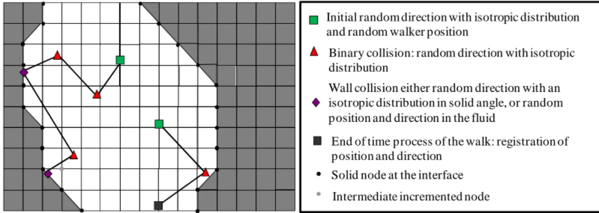
The random walk scheme is inspired from Burganos & Sotirchos and illustrated in figure 1.[24]
Here, the input 3D image has to be 8-bit grayscale and made up of cubic voxels (volumetric pixels), which are considered as grid cells. Before infiltration, the image is binarized (fluid/solid) and features two specific gray levels: 255 for the solid voxels and 0 for the fluid voxels. At the beginning of the simulation, each random walker, representing one or several molecules, is given initial coordinates and velocity. The representativity of a walker, i.e. the number of molecules it represents, is:
/walker) (molecules walk f n CV r= (5)
The value of the free path for each walker is equal to the free path of a single molecule and is sampled from a random deviate with decreasing exponential distribution. The particle will follow a straight line until the next collision with a solid wall or until free path exhaustion. The orientation distribution is isotropic in the bulk fluid and obeys a Knudsen cosine law on the walls. Whenever a walker hits a wall, a random number between 0 and 1 is drawn. Reaction is effective only if this number is lower than the chosen sticking probability.
Initial random direction with isotropic distribution and random walker position
Binary collision: random direction with isotropic distribution
Wall collision either random direction with an isotropic distribution in solid angle, or random position and direction in the fluid
End of time process of the walk: registration of position and direction
Intermediate incremented node Solid node at the interface
Figure 1: Scheme of the gas-kinetic random walker displacements in a 2D example
Whenever a walker sticks, the grey level of the closest fluid node is increased by I. The value of this increment ∆I represents the amount of solid volume generated by the number of
7
molecules embodied by one random walker. Therefore ∆I is determined by the ratio r defined
in eq. (5), the voxel volume Vvox and the solid molar volume υs.
vox walk f s vox s V n V C r V I . . . 255 255
υ
=υ
= ∆ (6)The node becomes solid when the grey level is at its maximum value 255. The surface is updated and a closed porosity detection routine, based on a front propagation algorithm, is performed; the closed porosity is then removed.
2.4. The surface and its evolution
The fluid/solid interface is extracted by a Simplified Marching Cube discretization.[25, 26] The
8-bit grayscale image is a regular grid of vertices, or cell summits. Each group of eight neighboring vertices forming a cubic cell is processed. The algorithm determines first whether the cube edges intersect the isosurface, which is defined by a threshold value. Intersections appear when vertices with values respectively above and below the threshold value are linked by an edge. The coordinates of intersection points are merged with the nearest solid vertex. They are then collected to constitute triangles according to a configuration list. Local values of porosity and internal surface area are associated with each configuration. Their global value can therefore be estimated by a loop on the entire image. Even though less accurate than a full Marching Cube technique, this method has the advantage of being extremely fast and
memory sparing.[26, 27] Agreement has been found with experimental values of surface area,
provided the sub-micrometric roughness contribution is not taken into account. Pore size distributions evaluated from X-ray tomographic data of C/C composites were in accordance
with experimental data from Hg intrusion curves.[28]
During infiltration simulation, a voxel will become solid only when his grey level exceeds 255. In this sense, this is a coarse Volume of Fluid approach, since the grayscale level of each voxel is considered as a filling ratio.
8
2.5. Computation of effective coefficients
The relevant properties are effective reaction rate and the diffusion tensor. These quantities are determined by running the simulation without morphological evolution and by the use of specific boundary conditions. Random walkers begin their evolution from two reservoirs connected to opposite faces of the image. Their mean concentration in each reservoir is regularly monitored and adjusted. The boundary conditions on the four remaining faces consist in translation and random replacement: a random walker reaching the image border is automatically shifted into a porous pixel on the opposite face, keeping the same distance with respect to the reservoirs. Mean periodicity of the concentration field is achieved in this way on non-periodic images without applying cell-to-cell constraints as in finite element or finite volume numerical solvers.
The reaction rate is easily obtained by counting the number of sticking events per unit time and volume, and the effective rate constant is extracted by division by the average concentration. The effective diffusivity is obtained like an effective conductivity in the heat transfer analogue. Imposing a difference of walker concentration between both reservoirs generates an overall gradient throughout the image. A row of the effective diffusivity tensor is
then determined by dividing the average diffusive flux components Ji by the concentration
gradient ∇iC after a steady state has been reached:
z y x j i C J C J D i j j i e ij , , , or ff = ∇ = ∇ = (7)
The flux is measured by counting the number of walkers reaching the border of the image (reservoirs not included) per unit time and cross-section. This numerical computation has to be repeated in directions x, y and z to get the full tensor.
9
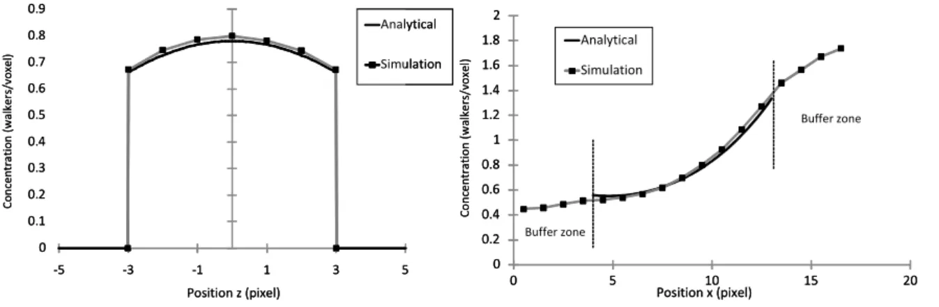
3. Validation
Validation has been carried out by considering the case of diffusion in a slit pore between two reactive plates, as shown in figure 2. Theoretical predictions of the concentration rate and of effective properties were established by considering (i) first order heterogeneous chemical reaction, (ii) isothermal process and (iii) a steady state situation for gas. Approximate analytical formulae have been obtained by solving a steady-state mass balance equation with appropriate boundary conditions and a single diffusion coefficient, which follows the
Bosanquet law [23].
Figure 2: Geometry of the validation case
3.1. Steady state concentrations
Figure 3 is an example of concentration profile in planes parallel to the plates and to the reservoirs. The sticking probability is equal to 10%. Other simulations for different values of this quantity were also in good agreement with the analytical solution, proving that the
algorithm can handle different gas consumption rates.[23]
0 0.1 0.2 0.3 0.4 0.5 0.6 0.7 0.8 0.9 -5 -3 -1 1 3 5
Concentration (walkers/ voxels)
Position z (pixel) Analytical Simulation C o n ce n tr a ti o n ( w a lk e rs /v o xe l) 0 0.1 0.2 0.3 0.4 0.5 0.6 0.7 0.8 0.9 -5 -3 -1 1 3 5
Concentration (walkers/ voxels)
Position z (pixel) Analytical Simulation C o n ce n tr a ti o n ( w a lk e rs /v o xe l) 0 0.2 0.4 0.6 0.8 1 1.2 1.4 1.6 1.8 2 0 5 10 15 20
Concentration (walkers/ voxel)
Position x (pixel) Analytical Simulation Buffer zone Buffer zone C o n ce n tr a ti o n ( w a lk e rs /v o x e l) 0 0.2 0.4 0.6 0.8 1 1.2 1.4 1.6 1.8 2 0 5 10 15 20
Concentration (walkers/ voxel)
Position x (pixel) Analytical Simulation Buffer zone Buffer zone C o n ce n tr a ti o n ( w a lk e rs /v o x e l)
10 Figure 3: Concentration profiles for a 10% sticking probability
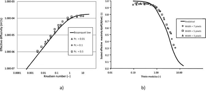
3.2. Effective properties
The diffusion tensor and the heterogeneous reaction rate were determined for various values of the mean free path and sticking probability. By this way, the evolution of these quantities with the Knudsen number and with the reaction/diffusion ratio has been followed. Figure 4 highlights the good agreement between numerical results and theoretical predictions.
1.00E-07 1.00E-06 1.00E-05 1.00E-04 1.00E-03 0.0001 0.001 0.01 0.1 1 10 Effective iffusioncoefficient (m²/s) Knudsen number (--) Bosanquet law Pc = 0.01 Pc = 0.1 Pc = 0.5 E ff e ct iv e d if fu si vi ty (m 2/s ) 1.00E-07 1.00E-06 1.00E-05 1.00E-04 1.00E-03 0.0001 0.001 0.01 0.1 1 10 Effective iffusioncoefficient (m²/s) Knudsen number (--) Bosanquet law Pc = 0.01 Pc = 0.1 Pc = 0.5 Bosanquet law Pc = 0.01 Pc = 0.1 Pc = 0.5 E ff e ct iv e d if fu si vi ty (m 2/s ) 0.01 0.10 1.00 10.00 S ca le d e ff e ct iv e re a ct iv it y k (e ff )/ k (h e t) ( -) Thiele modulus (-) Analytical Width = 7 pixels Width = 5 pixels Width = 3 pixels 0.0 0.1 0.2 0.3 0.4 0.5 0.6 0.7 0.8 0.9 1.0 0.01 0.10 1.00 10.00 S ca le d e ff e ct iv e re a ct iv it y k (e ff )/ k (h e t) ( -) S ca le d e ff e ct iv e re a ct iv it y k (e ff )/ k (h e t) ( -) Thiele modulus (-) Analytical Width = 7 pixels Width = 5 pixels Width = 3 pixels 0.0 0.1 0.2 0.3 0.4 0.5 0.6 0.7 0.8 0.9 1.0 a) b)
Figure 4: Evolution of effective diffusion coefficient (a) reaction rate (b)
We have checked that the effective diffusion coefficient does not depend on the reaction/diffusion ratio, as shown in previous work, but only on the Knudsen number,
verifying the Bosanquet law [29, 30]. On the other hand, we find that the effective
heterogeneous reaction rate is linked only to the local Thiele Modulus defined by:
eff het . D k L
σ
vφ
= (8), where
σ
v is the internal surface area.[31] The analytical and numerical results derived fromour study are similar to the curves obtained by Wood et al. in a similar diffusion-reaction study.[23, 32]
11
3.3. Infiltration indicator
The Thiele modulus highlights the operating conditions in which the infiltration is held. It characterizes the competition between chemical reaction and gas diffusive transport. Infiltration of the porous network is difficult if the value of the Thiele modulus is large. This configuration generally occurs towards the end of the densification process, when the open
porosity gradually becomes smaller, therefore diminishing the diffusion of the molecules.[33]
4. Applications
4.1. Densification of a carbon-fiber texture
In order to have a good representation of the C/C composite architecture, computerized micro-tomography (CMT) scans were performed at the European Synchrotron Radiation Facility (ESRF). The samples were raw and partly infiltrated C fiber preforms made of stacked satin weaves held together by stitching; they have been scanned with a 0.7 µm voxel edge size resolution, using the setup of the ESRF ID 19 beam line. Lower resolution scans (6.7µm/voxel) were also made on the same samples, in order to connect with a maximal confidence the fiber scale and larger scales, like the Representative Elementary Volume (REV) scale, which, for composite materials, may be larger than several millimeters.
The difference between the X-ray attenuation coefficients of the carbon fibers, the carbon matrix, the embedding matrix and air is small. The contrast between these phases is therefore relatively faint. Two approaches are then possible: first, the complete refraction index reconstruction, called holotomography, and second, the phase-contrast edge-detection mode,
associated to image processing for the segmentation of the constitutive phases.[34] Details on
the experimental procedure have been given in previous studies.[35, 36]
The algorithm requires binary images: fibers in white (grey level 255) and the void in black (grey level 0). In order to do so, specific segmentation tools have been developed. For instance, Martín-Herrero and Germain have designed and successfully tested an algorithm
12
based on a differential profiling method.[37] Intensity edges are detected on every 2D cross
section parallel to the reference system and are refined by correlating the outputs in 3D. A “heavy-ball” procedure is then used: fibers are individuated by simulating the trajectory of a ball within them. It considers, at each step, the previous move (inertia) and the best overlapping between the ball volume and the fiber voxels (to keep the ball inside the fiber). Another method uses directly the image gradient (and principally the edge-enhancement patterns) for the estimation of the localization of fiber axes; once the axes have been isolated, a gradient sensitive region-growing procedure may be applied for the segmentation of the
fibers first and then of the matrix.[38]
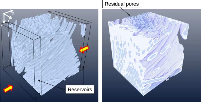
Figure 5 shows the progression of carbon matrix deposition on a 300x300x300 voxel
(0.21x0.21x0.21mm3) image of the fibrous preform. The sticking probability is equal to 16%
and the simulation carried out in a relatively rarefied diffusion regime (Kn = 8). This is a typical set of parameters in practical implementations of the process; however, depending on the precise nature of the reactants, the sticking coefficient may be either larger (e.g. for radical species) or lower. Here, the value has been chosen in order to illustrate the rarefaction effects at pore-scale.
The main difficulty during CVI is to use sufficiently reactive operating conditions in order to obtain a reasonable deposit rate. But depositing with a high reactivity generates a premature obstruction of the preform surface in contact with the reservoirs (which directions are shown with the arrows), leaving an uncoated stack of fibers in the heart of the composite. This phenomenon is clearly visible during this study. Computing with a lower value of sticking probability would delay this event by allowing a more homogeneous repartition of the random walkers. The formation of carbon matrix (called pyrocarbon) is usually performed with lower sticking probabilities than the one used in this example.
13 Reservoirs Residual pores x y z Reservoirs Residual pores x y z
Figure 5: Matrix deposition simulation on a 300×300×300 voxel image: left initial raw preform right final infiltrated composite. Reservoirs are materialized by the arrows.
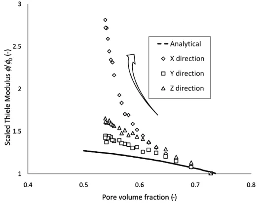
Figure 6 shows the evolution of the scaled Thiele modulus in all three directions of the image. This quantity is defined by:
eff 0 0 0 . . D D v v
σ
σ
φ
φ
= (9), where σv0 is the initial internal surface area and D0 the initial diffusion coefficient. The
theoretical evolution of this quantity is roughly proportional to the inverse square root of the mean pore diameter. The linear evolution of the Thiele modulus according to the directions not in contact with the reservoirs is respected. The increase in the third direction becomes more and more important when the percolation threshold is close. The value of this threshold is a function of the geometry of the porous medium but also of the deposition rate and of the initial Knudsen number. From the point of view of material homogeneity, the best infiltration would be achieved for extremely low sticking probabilities and Knudsen numbers, which
correspond to the slowest reaction rates.[39] Numerically, these conditions are faster simulated
by a mathematical dilatation of the preform image: the matrix grows everywhere with the same linear speed around the fibers. A cylindrical fiber remains cylindrical, but its radius
14
grows. Fast Marching methods are a solution for this type of simulation on non-analytical surfaces.[40] 1 1.5 2 2.5 3 0.4 0.5 0.6 0.7 0.8 ScaledThieleModulus( -)
Pore volume fraction (-) Analytical X direction Y direction Z direction S ca le d T h ie le M o d u lu s φ / φ0 (-) 1 1.5 2 2.5 3 0.4 0.5 0.6 0.7 0.8 ScaledThieleModulus( -)
Pore volume fraction (-) Analytical X direction Y direction Z direction S ca le d T h ie le M o d u lu s φ / φ0 (-)
Figure 6: Evolution during the simulation of the scaled Thiele modulus. The arrow indicates the direction of
increasing time.
4.2. Deposition on a structured wafer
Validation of the present simulation approach should also account for 2D-like systems description. CVI is a variation of the Chemical Vapor Deposition process that is notably used for the preparation of electronic components; Plasma Enhanced Chemical Deposition is a closely related process, even when applied to simple geometries. In the context of microelectronics device preparation, the sacrificial layer method for example implies the use
of silicon oxide or silicon nitride gaseous precursors.[41] Recently, a Remote Plasma Enhanced
Chemical Deposition (RPECVD) method was applied in such an aim using
TetraMethylDiSilOxane (TMDSO) as a precursor.[42, 43] Deposition of 20 to 50 µm-thick films
was accomplished. At feature scale, the impact of surface irregularities during RPECVD has been evidenced, even though the deposit thickness is neatly larger than the size of the
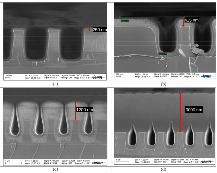
15
irregularities. The use of structured wafer shows the evolution of the layer grown in a trench. The figures 7a,b,c and d show the evolution of the shape of layers with reference thicknesses of 250, 415, 1200 and 3000 nm, respectively. These figures make evidence of the arising of knobs, i.e., smooth and cylindrical hill-type irregularities once the trench was filled (fig.7d). [43]
This complex behavior, shown for illustration, is not yet well understood.
250 nm 250 nm 415 nm 415 nm (a) (b) 1200 nm 1200 nm 3000 nm3000 nm (c) (d)
Figure 7: SEM micrographs of ppTMDSO films deposited in trenches on Si substrate. The films thicknesses on
directly exposed planar surfaces are (a) 250, (b) 415, (c) 1200 and (d) 3000 nm, respectively, as indicated by the
16
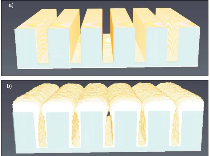
Numerical simulations on similar trench shapes have been carried out; an example result (Kn = 5, Pc = 0.26) is shown in figure 8. The correct qualitative agreement between figs 7b and 8b is an encouraging result. a) b) a) b) a) b)
Figure 8: Simulation of deposition in parallel trenches where Kn =5 and Pc = 25%. a) Initial geometry; b) after
deposition.
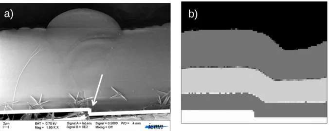
In order to propose a possible simulation of the present RPECVD-induced TMDSO polymerization, we have considered another case related to these statements. Figure 9a shows
the overgrowth following the deposition on a wafer presenting a 1µm-step. An analysis of the
deposition rate and conditions leads to an estimate of the sticking probability lying close to 26% and of the Knudsen number (where the reference length is now the step height) close to
17
mass flux, as obtained by the kinetic theory of gases. A simulation was undertaken with these parameters on a 100x100x100 voxel image. A reservoir containing walkers in constant concentration is located on the upper face of the image, and pseudo-periodic boundary conditions were applied on the other faces. Gradual deposition is shown in figure 9b.
a)
b)
a)
b)
Figure 9 a) Deposition of TMDSO on plane substrate with a step like asperity (marked by a white arrow)
b) Simulated evolution of deposit on the step.
The initial step is visible throughout the deposition process but becomes more and more distorted. The final morphology is not exactly the same as shown in figure 8a: no clear overgrowth is obtained. This seems to indicate that the numerical model does not take enough physico-chemical phenomena into account. Among possible overgrowth causes to be investigated in the future we can list: non-linear deposition kinetics; complex homogeneous reactions; polymer creep under thermal stresses during or after deposition. Surface diffusion is one of the phenomena that we have not taken into account; however its usual effect is to smooth away the sharp edges, particularly the reentrant ones. This is not observed in the case illustrated by fig. 9a. However it could play some role in other application cases and its inclusion in the numerical tool is currently under consideration.
18
5. Conclusion
A complete numerical scheme for the local scale modeling of CVI and CVD based on 3D representations of the substrates has been presented. The algorithm is based on a Monte Carlo random walk method where the surface is meshed according to a specific discretization scheme, allowing instant modification during the random walk. The developed tool is capable not only of performing a deposition simulation but also of determining the effective diffusion tensor and reaction rate of the medium. The computation of these effective properties is motivated by a multi-scale approach of the modeling of CVI. The algorithm was validated by confronting numerical results with theoretical solutions in the case of diffusion and reaction through a slit pore. Concentration rates as well as effective properties in all diffusion regimes were in good agreement with their analytical predictions. Fiber-scale densifications on tomographic images of actual fiber arrangements enabled to illustrate typical CVI phenomena. This numerical tool can also perform RPECVD deposition on structured substrates and highlight the effects of asperities at a local scale.
Ongoing improvements include the introduction of non-linear deposition kinetics (second order, Langmuir-Hinshelwood, etc) and surface diffusion. Also, program optimization for very low sticking probabilities is under way.
Acknowledgements
The authors wish to thank the French Ministry for Education & Research as well as SAFRAN- Snecma Propulsion Solide for PhD funding to W. Ros. They are also indebted to the CNRS research group GdR 3184 “SurGeCo” for initiating the collaboration between all partners.
19
References
[1] W. Krenkel: Ceramic Matrix Composites, Wiley-VCH, Weinheim 2008. [2] G. Savage: Carbon/Carbon composites, Chapman & Hall, London 1993.
[3] E Fitzer, L. Manocha: Carbon reinforcements and carbon/carbon composites, Springer, Berlin 1998.
[4] E. Bouillon, P. Spriet, G. Habarou, C. Louchet, T. Arnold, G. Ojard, D. Feindel, C. Logan, K. Rogers, D. Stetson, Procs, ASME Turbo Expo, 2004, 53976.
[5] H.C. Mantz, D.A. Bowers, F.R. Williams, M.A. Witten, Procs, IEEE 13th Symposium on
Fusion Engineering, 1990, 2, 947.
[6] A. Essakhi, A. Lögberg, P. Supiot, B. Mutel, S. Paul, V. Le Coutois, V. Meille, I. Pitault, E. Bordes-Richard, Studies in Surface Science & Catalysis 2010, 175, 17.
[7] S. Békri, J-F. Thovert, P-M. Adler, Chem. Eng. Sci. 1995, 50, 2765. [8] D.A. White, N. Verdone, Chem. Eng. Sci. 2000, 55, 2213.
[9] I. Gaus, M. Azouaral, I. Czernichowski-Lauriol, Chem. Geology 2005, 217, 319.
[10] G.L Vignoles, C. Gaborieau, S. Delettrez, G. Chollon, F. Langlais, Surf. Coat. Technol, 2008, 510.
[11] G. Kokkoris, E. Gogolides, A.G. Boudouvis, Microelectronics Eng, 2000, 599. [12] E.E. Petersen, AIChE, 1957, 3.
[13] R. Fédou, F. Langlais, R. Naslain, J. Mater. Synth. & Proc, 1993, 1, 43. [14] J.Y. Ofori, S.V. Sotirchos, Ind. Eng. Chem. Res, 1996, 35, 1275.
[15] J.Y. Ofori, S.V. Sotirchos, J. Electrochem. Soc, 1996, 6, 1962. [16] W. Zhang, K.J. Hüttinger, Carbon, 2001, 39, 1013.
[17] A. Li, K. Norinaga, W. Zhang, O. Deutschmann, Comp. Sci. & Technol, 2008, 166, 1097. [18] T-A. Langhoff, E. Schnack, Chem. Eng. Sci, 2008, 63, 3948.
20
[20] G.L. Vignoles, O. Coindreau, W. Ros, I. Szelengowicz, C. Mulat, C. Germain, M. Donias, Adv. Sci. & Technol. 2010, 71, 108.
[21] K. Pearson, Nature 1905, 72, 342.
[22] L.B. Loeb, J. Am. Chem. Soc., 1959, 81, 1267
[23] G.L. Vignoles, W. Ros, C. Mulat, O. Coindreau, C. Germain, Comput. Mater. Sci 2011, 50, 1157.
[24] V. N. Burganos, S. V. Sotirchos, Chem. Eng. Sci 1989, 44, 2451. [25] G.L. Vignoles, J. Phys. IV France, 1995, C5, 159.
[26] G.L. Vignoles, M. Donias, C. Mulat, J.-F. Delesse, C. Germain, Comput. Mater. Sci. 2011, 50, 893.
[27] W.E. Lorensen, H.E. Cline, ACM SIGGRAPH, 1987, 163.
[28] O. Coindreau, G.L. Vignoles, J.-M. Goyheneche, Ceram. Trans. 2005, 175, 71. [29] D. Ryan, R.G. Carbonell and S. Whitaker, Chem. Eng. Sci. (1980), 35, 10.
[30] W.G. Pollard, Physical Review 1948, 73, 732. [31] E.W. Thiele, Ind. Eng. Chem. 1939, 31, 916.
[32] B. D. Wood, M. Quintard, S. Whitaker, Chem. Eng. Sci 2000, 55, 5231.
[33] G.L. Vignoles, O. Coindreau, C. Mulat, C. Germain, J. Lachaud, 2010, Adv. Eng. Mater. n/a, DOI: 10.1002/adem.201000233.
[34] P. Cloetens, W. Ludwig, J. Baruchel, D. Van Dyck, J. Van Landuyt, J. P. Guigay, M. Schlenker, Appl. Phys. Lett. 1999, 75, 2912.
[35] O. Coindreau, P. Cloetens, G.L. Vignoles, Nucl. Instr. and Meth. in Phys. Res. B 2003, 200, 295.
[36] O. Coindreau, G. L. Vignoles, J. Mater. Res. 2005, 20 2328. [37] J. Martín-Herrero, C. Germain, Carbon 2007, 45 1242.
21
[38] C. Mulat, M. Donias, P. Baylou, G.L. Vignoles, C. Germain, J. Electronic Imaging, 2008, 17, 0311081.
[39] G.L. Vignoles, C. Germain, O. Coindreau, C. Mulat, W. Ros, ECS Transactions 2009, 25, 1275.
[40] J.A. Sethian: Level Set Methods, Cambridge University Press, 1996.
[41] B.A. Peeni, M.L. Lee, A.R. Hawkins, A.T. Wooley, Electrophoresis, 2006, 27, 4888. [42] P. Supiot, C. Vivien, A. Granier, A. Bousquet, A. Mackova, F. Boufayed, D. Escaich, P. Raynaud, Z. Stryhal, J. Pavlik, Plasma Processes and Polymers, 2006, 3, 100.
[43] A. Abbas, P. Supiot, V Mille, D Guillochon and B. Bocquet, Journal of Micromechanics
22
Nomenclature
Parameters Meaning Unit
c Gas-phase concentration of reactant mol/m3
c Mean concentration mol/m3
D Species binary diffusivity in pure gas m2/s
Deff Effective species diffusivity in porous medium m2/s
dp Pore diameter m
H Half distance between reactive plates m
J Average diffusive flux mol/m2/s
khet Heterogeneous reaction rate constant m/s (if linear)
keff Effective (homogenized) heterogeneous reaction rate
constant 1/s (if linear)
k~ Effective reaction constant -
Kn Knudsen number -
L Porous medium thickness m
M Molar mass kg/mol
A
N Avogadro constant 1/mol
nwalk Number of walkers -
p Pressure Pa
Pc Sticking probability -
r Nb. of gas moles per walker mol
R Perfect gas constant J/mol/K
T Temperature K
<v> Mean molecular velocity m/s
Vf Fluid volume m3
Vvox Voxel volume m3
I Grey level increase -
<λ> Molecular mean free path m
σc Molecular collision cross section m
σv Internal surface area 1/m
23
Φ Thiele modulus -