HAL Id: hal-00630459
https://hal.archives-ouvertes.fr/hal-00630459
Submitted on 10 Oct 2011
HAL is a multi-disciplinary open access
archive for the deposit and dissemination of sci-entific research documents, whether they are pub-lished or not. The documents may come from teaching and research institutions in France or
L’archive ouverte pluridisciplinaire HAL, est destinée au dépôt et à la diffusion de documents scientifiques de niveau recherche, publiés ou non, émanant des établissements d’enseignement et de recherche français ou étrangers, des laboratoires
Competitive Growth in a Life-cycle Model: Existence
and Dynamics
Hippolyte d’Albis, Emmanuelle Augeraud-Véron
To cite this version:
Hippolyte d’Albis, Emmanuelle Augeraud-Véron. Competitive Growth in a Life-cycle Model: Existence and Dynamics. International Economic Review, Wiley, 2009, 50 (2), pp.459-484. �10.1111/j.1468-2354.2009.00537.x�. �hal-00630459�
Competitive Growth in a Life-cycle Model:
Existence and Dynamics
∗
Hippolyte d’ALBIS
†Toulouse School of Economics (LERNA)
Emmanuelle AUGERAUD-VÉRON
‡LMA, University of La Rochelle
This version: September 23, 2007
First version: February 25, 2006
Abstract
In this paper, the dynamic behavior of the capital growth rate is ana-lyzed using an overlapping-generations model with continuous trading and finitely lived agents. Assuming a technology satisfying constant social returns to capital, the equilibrium growth rate is piecewise-defined by functional differential equations with both delayed and ad-vanced terms. The main result concerns the existence of a solution expressed as a series of exponentials, which is shown to crucially de-pend on the initial wealth distribution among cohorts. Upon existence, the dynamics of the capital growth rate has a saddle-point trajectory that converges to a unique steady-state. Along the transition path, the growth rate exhibits exponentially decreasing oscillations.
JEL Classification: D50, D90.
Keywords: Overlapping-generations Models, Endogenous Growth, Functionnal Differential Equations of Mixed Type.
∗We thank two anonymous referees as well as A. d’Autume, E. Benoit, J-P. Drugeon,
O. Licandro, B. Wigniolle, and participants at the Conference on Irregular Growth (Paris, 2003) and the Workshop on Dynamic Macroeconomics (Vigo, 2003) for stimulating sug-gestions and comments. The usual disclaimer applies.
†Correspondence: Université de Toulouse I, 21 allée de Brienne, 31000 Toulouse,
France. Phone/fax: 33-5-6112-8876/8520. E-mail: [email protected]
‡Correspondence: LMA, Université de La Rochelle, Avenue Michel Crépeau, 17042 La
1
Introduction
As they deal with population or social security issues, applied studies have come to use settings that encompass an arbitrarily large number of over-lapping generations of individuals to ease the confrontation with real world annual data. Among them, Auerbach and Kotlikoff [3] notably propose a de-terministic framework and Rios-Rull [19] a stochastic one. Such models are unfortunately at odds with the benchmark structure of the theoretical liter-ature based upon two periods overlapping generations of individuals. Recent contributions, such as Kehoe et al. [15], have thus been aimed at developing a fruitful analysis of large-square models and exhibited specific conditions on the dynamic properties of equilibrium paths. However, a limit to their use on a wide spread basis springs from the difficulties that emerge in the course of their analytical resolution. Our paper introduces a simple method that allows for solving models with a continuum of overlapping generations. It also proposes a complete resolution in a specific case which provides new insights on the existence and convergence properties of equilibrium paths.
In models with many overlapping generations, the dynamics of endoge-nous variables depends on a finite number of their past and future realiza-tions. This dependency creates the analytical difficulty of these models. In discrete time frameworks, the analysis of the dynamics requires the study of polynomials, whose order increases with the number of generations, and which will not be tractable in the general cases. We claim that this diffi-culty may however be circumvented using the continuous time framework developed by Cass and Yaari [10]; in a nutshell, it eases the mathematical
resolution without affecting the qualitative analysis. However, in continuous time frameworks, the dynamics is characterized by a functional differential equation of mixed type (MFDE), i.e. the dynamics is affected by distributed delays and advances. We propose an integrated treatment of such a structure in a simple competitive equilibrium case considering an overlapping genera-tions model with production in which the technology exhibits constant social returns to capital. Capital dynamics is hence described by an MFDE that happens to be linear, and allows for a global dynamics analysis.
We prove that, upon existence of a competitive path, the growth rate has a transitional dynamics and converges to a steady state through exponen-tially decreasing oscillations. The oscillatory behavior is now a well known output of dynamic systems with delays. As pointed out by Boucekkine, de la Croix and Licandro [6], they appear as resulting from the vintage human capital structure. Recently, Demichelis and Polemarchakis [11] and d’Albis and Augeraud-Véron [1] have also been find a related class of fluctuations. However, as for the existence problem, there is to our knowledge, few papers that have studied it. Rustichini [20] has claimed that MFDE may fail to have a solution while Burke [9] has proven that the existence of an equilibrium is not always ensured in continuous-time overlapping generations models even under rather standard and simple assumptions.
Our main result is a theorem of existence of an intertemporal equilibrium. We proceed by studying the existence of a strictly positive and bounded solu-tion to the MFDE. We show how to use the piecewise definisolu-tion of the capital dynamics to define the set of initial distributions of wealth that ensure the existence of the equilibrium. This result points out the importance of
ini-tial conditions: not all iniini-tial wealth distributions among the generations are compatible with the existence of an equilibrium. Some distributions may indeed generate short run fluctuations whose magnitude is so large that they would lead to negative aggregate assets. As a consequence, when macroeco-nomic variables oscillate, initial distributions matter.
The paper is organized as follows. In section 2, we present the basic framework of the model and determine the functional equations that char-acterize the capital dynamics at the equilibrium. In section 3, we analyze the global dynamics and propose an existence theorem based on the initial wealth distribution. We conclude in section 4.
2
The model
This section develops an overlapping-generations model with continuous trad-ing and finitely-lived individuals. Assumtrad-ing a technology with constant re-turns to capital, it characterizes the capital dynamics of such an economy.
2.1
Individual behavior
Time is continuous and has a starting point denoted τ ∈ R; let t denotes the time index such that t ≥ τ. Individuals live for an interval of time of length ω > 0. In what follows, the lifespan is considered as finite although the limit case of an infinite horizon (ω → +∞) can be computed for discussion purposes. It is assumed that individuals only derive utility from consumption and that they have isoelastic preferences and a non negative time discount denoted ρ. Let c (s, t) ≥ 0 denotes the real consumption of an individual who born at time s as of time t. Hence, the intertemporal utility of an individual
who born at time s ∈ (τ − ω, t], denoted u (s, t), satisfies: u (s, t) = Z s+ω t e−ρ(z−t)v (c (s, z)) dz, (1) where: v (c) = ¯ ¯ ¯ ¯ ¯ ¯ ¯ c1−1σ−1 1−1σ if σ 6= 1, ln c if σ = 1, (2)
with σ > 0 standing for the elasticity of intertemporal substitution. Dur-ing a lifetime, the labor supply is fixed and equal to 1 and w (t) , an age-independent labor income is received. Individuals have access to competitive capital markets that yield the risk-free interest rate r (t). Let a (s, t) denotes the real wealth of an individual who born at time s as of time t. The instan-taneous budget constraint is therefore for all t ≥ τ:
∂a (s, t)
∂t = r (t) a (s, t) + w (t)− c (s, t) . (3) Individuals enter the economy with no financial assets except those who are alive at the initial date of the economy and which are endowed with a given financial wealth. Therefore, initial conditions write:
a (s, τ ) given if s ∈ (τ − ω, τ) , a (s, s) = 0 if s ≥ τ.
(4)
Finally, individuals cannot die indebted. Hence, for s > τ − ω, terminal constraints write:
a (s, s + ω)≥ 0 if ω ¿ +∞, limz→+∞e−Uszr(u)dua (s, s + z)≥ 0 if ω → +∞.
(5)
Moreover, assume that a (s, t) and c (s, t) are C1((τ
− ω, ∞) × (τ, ∞)) while r (t) and w (t) are continuous for all t ∈ (τ, ∞).
The individual program is to maximize (1) subject to (3), (4) and (5). The optimal consumption behavior is given in the following lemma.
Lemma 1 For (s, t) ∈ (τ − ω, τ) × (τ, s + ω), the optimal consumption sat-isfies: c (s, t) = a (s, τ ) e Ut τr(u)du+Rs+ω τ w (z) e Ut zr(u)dudz Rs+ω τ e Ut z[(1−σ)r(u)+σρ]dudz , (6) and for (s, t) ∈ (τ, ∞) × [s, s + ω): c (s, t) = Rs+ω s w (z) e Ut zr(u)dudz Rs+ω s e Ut z[(1−σ)r(u)+σρ]dudz . (7)
Proof. See the Appendix.
As initial conditions (4) differ, it is necessary to distinguish individuals who were alive at time t = τ , and whose behavior is affected by the initial wealth distribution, from those who born at time t > τ . Moreover, equations (6) and (7) show that the optimal consumption is a function of the past and anticipated factor prices all along the individual’s life-cycle. Hence, in the case of an infinite lifespan obtained as ω → +∞, it is the entire path of prices starting at the birth date that affects the individual behavior.
2.2
Aggregate dynamics
The demographic structure is in overlapping generations and the population is stable. Each individual belongs to a cohort composed of a continuum of identical individuals; the size of cohort born at time s as of time t ∈ [s, s + ω), is βN (s) where β > 0 is the birth rate and N (s) is the size of the population at time s. At each point of time, a new cohort enters the population while
the oldest one leaves it. For all t ≥ τ, N (t) satisfies:
N (t) = Z t
t−ω
βN (s) ds. (8)
The demographic growth rate, denoted n, is obtained by replacing N (t) = N (s) en(t−s) in (8) and then solving the following equation:
Z ω
0
βe−nαdα = 1. (9)
The macroeconomic counterpart of any individual variable is obtained by integrating it on the birth date over an interval of length ω. Hence, the aggregate assets per head, denoted a (t), satisfy for all t ≥ τ:
a (t) = Z t
t−ω
βe−n(t−s)a (s, t) ds. (10)
Differentiating (10) with respect to time and using the individual budget constraints yields the following standard dynamics:
da (t)
dt = [r (t)− n] a (t) + w (t) − c (t) , (11) where c (t) denotes the aggregate consumption per head such that:
c (t) = Z t
t−ω
βe−n(t−s)c (s, t) ds. (12)
Remark that for t ∈ (τ, τ + ω), the population is composed of cohorts born before and after t = τ , while for t ∈ (τ + ω, ∞), it only remains cohorts born after the initial date τ . Using (6) and (7), c (t) hence writes:
c (t) = Z τ t−ω βe−n(t−s)a (s, τ ) e Ut τr(u)du+Rs+ω τ w (z) e Ut zr(u)dudz Rs+ω τ e Ut z[(1−σ)r(u)+σρ]dudz ds + Z t τ βe−n(t−s) Rs+ω s w (z) e Ut zr(u)dudz Rs+ω s e Ut z[(1−σ)r(u)+σρ]dudz ds, (13)
if t ∈ (τ, τ + ω) and: c (t) = Z t t−ω βe−n(t−s) Rs+ω s w (z) e Ut zr(u)dudz Rs+ω s e Ut z[(1−σ)r(u)+σρ]dudz ds, (14)
if t ≥ τ + ω. As a consequence, the aggregate dynamics is generically piecewise-defined. Exceptions are obviously the limit case of an infinite lifes-pan (ω → +∞) where only (13) holds, and the limit case of no initial date for the economy (τ → −∞) where it is only (14) that characterizes the dy-namics. Remark that the piecewise definition, which will be crucial for the existence result presented section 3, is not considered in related works on continuous-time OLG model such as Demichelis and Polemarchakis [11] and d’Albis and Augeraud-Véron [1] who focus on the asymptotic dynamics.
Moreover, equations (13) and (14) show that the aggregate consumption at time t is determined by the path of factor prices on the interval (τ , t + ω) when t belongs to (τ , τ + ω) and on the interval (t − ω, t + ω) when t ≥ τ +ω. It is important to notice that the dynamics of the aggregate consumption at time t is also affected the same path of prices, which implies that the dynamics is characterized by functional differential equations. Indeed, differentiating (12) with respect to time yields:
dc (t)
dt = [σ (r (t)− ρ) − n] c (t) + βc (t, t) − βe
−nωc (t− ω, t) , (15)
where individual consumptions at the beginning and the end of the life-cycle are immediately computed with (6) and (7) such as:
c (t, t) = Rt+ω t w (z) e Ut zr(u)dudz Rt+ω t e Ut z[(1−σ)r(u)+σρ]dudz , (16)
and: c (t− ω, t) = ¯ ¯ ¯ ¯ ¯ ¯ ¯ ¯ ¯
a(t−ω,τ )eU tτ r(u)du+Uτtw(z)eU tz r(u)dudz Ut τe U t z [(1−σ)r(u)+σρ]dudz if t ∈ [τ, τ + ω) , Ut t−ωw(z)e U t z r(u)dudz Ut t−ωe U t z [(1−σ)r(u)+σρ]dudz if t ≥ τ + ω. (17)
The dynamics of c (t) given by (15) decompose itself in three terms. The first one is the usual difference between the individual consumption growth rate, σ (r (t)− ρ), and the population growth rate, n. Aggregate consumption per head is likely to increase when the first is greater than the second. The second term, which was initially pointed out by Blanchard [5] and Weil [22], is the initial consumption of the newborns, c (t, t). They enter the economy at rate β and make the aggregate consumption increase. By considering individuals with infinite horizons, the two authors obtain a consumption of the newborns that reduces to a function of variables characterized for time t. This is not anymore true when ω is finite. Differentiating (16) with respect to t yields a dynamics that depends on future prices:
dc (t, t) dt = ( σ [r (t)− ρ] + 1− e Ut t+ω[(1−σ)r(u)+σρ]du Rt+ω t e Ut z[(1−σ)r(u)+σρ]dudz ) c (t, t) +w (t + ω) e Ut t+ωr(u)du− w (t) Rt+ω t e Ut z[(1−σ)r(u)+σρ]dudz , (18)
while the infinite horizon case reduce to: dc (t, t) dt ¯ ¯ ¯ ¯ ω→+∞ = σ [r (t)− ρ] c (t, t) + R+∞c (t, t)− w (t) t e Ut z[(1−σ)r(u)+σρ]dudz , (19)
provided that r (z) > max {0, σρ/ (σ − 1)} for z ∈ [t, +∞). Remark notably with (18), that the wage at time t + ω, w (t + ω) , affects the consumption of the newborn of date t, while it does not influence the consumption of
individuals born before date t. Finite horizons thus create a discrete advance in the aggregate dynamics.
The third term that influence the dynamics of c (t) given by (15) corre-sponds to the last consumption, c (t − ω, t), of those who leave the economy at rate βe−nω. This term is obviously linked to the assumption of finite
lifespan and therefore does not appear in Blanchard [5] and Weil [22]. The level and the dynamics of c (t − ω, t) depend on past prices. Nevertheless, it is important to remark with (17) that c (t − ω, t) can be rewritten for t ∈ (τ, τ + ω) as a function of variables characterized at time t. After that initial interval of time, the dynamics is affected by delayed variables. Indeed, one has: dc (t− ω, t) dt = ( σ [r (t)− ρ] + e Ut t−ω[(1−σ)r(u)+σρ]du− 1 Rt t−ωe Ut z[(1−σ)r(u)+σρ]dudz ) c (t− ω, t) +w (t)− w (t − ω) e Ut t−ωr(u)du Rt t−ωe Ut z[(1−σ)r(u)+σρ]dudz , (20)
if t ≥ τ + ω. The wage at time t − ω, w (t − ω) , affects the consumption of individual born at date t − ω, while it does not influence the consumption of individuals born after date t. The finite lifespan assumption hence creates a discrete delay in the aggregate dynamics as of time t ≥ τ + ω. Conversely, before date τ + ω, their are only cohorts born before date τ that die, and consequently, there is no past value of factor prices that becomes unrelevant for the aggregate dynamics. To summarize, the aggregate dynamics is in-fluenced by discrete advances for t ∈ (τ, τ + ω) and by both advances and delays for t ≥ τ + ω.
2.3
Intertemporal equilibrium
Assume there is a unique material good, whose price is normalized to 1. It can be used for consumption or for adding to the capital stock. This good is produced by many competitive firms whose aggregate activity is described by a production function with labor L (t) and capital K (t) as inputs. The aggregate production is supposed to satisfy:
Y (t) = A (K (t))α(e (t) L (t))1−α, (21)
where e (t) is an externality from the producer perspective and where A > 0 and α ∈ (0, 1). The capital depreciation rate is constant and denoted δ ≥ 0. For all t ≥ τ, factor prices equal marginal products:
r (t) + δ = αA (K (t))α−1(e (t) L (t))1−α, (22) w (t) = (1− α) A (K (t))α(e (t))1−α(L (t))−α. (23)
Define the aggregate capital per head as k (t) = K (t) /L (t). To close the model, assume that the externality is of the "learning-by-doing" type and thus satisfies at the equilibrium the following equality: e (t) = k (t).
Definition An equilibrium with perfect foresight is a function k (t) , t ≥ τ, that belongs to R+
, is continuous and has bounded variations on (τ , ∞) such that (i) individuals maximize their utility subject to the budget constraints, (ii) firms maximize their profits, (iii) markets clear, and (iv) e (t) = k (t).
cumula-tive functions of past capital stock: y (t) = Z t τ k (z) e−r(z−t)dz, (24) v (t) = β (1− α) A Rt τ k (z) Rt z e−γ(t−s)e−r(z−s)dsdz Rω 0 e−µzdz , (25) ˜ v (t) = β (1− α) A Z t τ k (z) Z t z e−γ(t−s)e−r(z−s) Rs τ e−µ(u−s)du dsdz. (26)
where r = αA − δ, γ = n − σ (r − ρ) and µ = r − σ (r − ρ). Then, the equilibrium is characterized in the next Lemma.
Lemma 2 The equilibrium is the solution of the following system: dv (t) dt = −γv (t) + β (1− α) A Rω 0 e−µudu y (t) , (27) d˜v (t) dt = −γ˜v (t) + β (1− α) A Rτ −t 0 e−µudu y (t) , (28) dy (t) dt = ry (t) + k (t) , (29) dk (t) dt = (A− δ − n) k (t) − z (t) + e −nωv (t)˜ − e−σ(r−ρ)ωe−γ(t−τ)˜v (τ + ω) +v (t)− e−rωv (t + ω) + e−rωe−γ(t−τ)v (τ + ω) , (30) if t ∈ (τ, τ + ω) and of (27), (29) and: dk (t) dt = (A− δ − n) k (t)+ ¡ 1 + e−(γ+r)ω¢v (t)−e−γωv (t− ω)−e−rωv (t + ω) , (31) if t ≥ τ + ω. In addition, z (t) , t ∈ (τ, τ + ω) and k (τ) > 0 are given.
Proof. See the Appendix.
As explained previously, the dynamics is piecewise-defined: as the economy is supposed to have a finite starting point, a first system of equations char-acterizes the capital dynamics as long as it exists individuals who were alive
at the initial date; this system includes, in variable z (t), the initial distri-bution of wealth among generations which constitutes the initial condition of the system. The capital dynamics, given by (30), is characterized by a differential equation with discrete advances. When all the individuals who were alive at the initial date, have died, a second system of equations then characterizes the dynamics for an infinite future. The capital dynamics, then given by (31), is characterized by a differential of mixed type (MFDE): delays and advances influence the dynamics. It is easy to check that the two system are the same for t = τ + ω.
Moreover, the bounded life-span assumption is crucial: we show in the next corollary, that when ω goes to infinity, the dynamics is define by a single system of ordinary differential equations.
Corollary 1 Suppose that n > 0 and µ > 0. When ω → +∞, the equilib-rium is the solution of (27), (29) and:
dk (t)
dt = (A− δ − n) k (t) − nµe
−γ(t−τ)k (τ ) + v (t) , (32)
for all t ≥ τ and with k (τ) > 0 given.
Proof. See the Appendix.
It is important to notice that the linearity of the dynamics crucially de-pends on the assumption of constant social returns to capital. The dy-namics would be non linear by replacing the learning-by-doing assumption by, for instance, an exogenous labor augmenting technical progress such as: e (t) = e (τ ) eg(t−τ), with g > 0. Linearizing on the neighborhood of a
there is no Hopf bifurcations, the dynamics is likely to be qualitatively sim-ilar to the one that is to be studied in the next section. On such issue, we refer to the pioneer article proposed by Cass and Yaari [10] who study a non linear dynamics in the case of a specific neoclassical production function, and to recent developments by d’Albis and Augeraud-Véron [1] and [2] and Hupkes and Verduyn Lunel [14]. However, when the dynamics is non linear, the existence problem studied below, that relies on the dynamics behavior on the initial interval of time is still an open question.
3
The results
This section proposes a complete study of the global dynamics. In a first part, we use rather standard tools to analyze the dynamic behavior after some initial interval of time. The results obtained are then similar to those proposed by recent related contributions. The real novelty of the paper lies in the second part of the section, where we propose an existence theorem that uses the dynamics during the initial interval of time.
3.1
Capital dynamics for
t
≥ τ + ω
Let us first ignore the initial dynamics and study the capital behavior for t ≥ τ + ω. We proceed by analyzing the roots of the corresponding characteristic equation.
Lemma 3 Let r = αA − δ. The characteristic equation associated to the system of equations (27), (29) and (31) has:
2) no complex roots with real part that belong to the closed strip:
[min{r − n, ¯g} , max {r − n, ¯g}] ,
except ¯g itself;
3) an infinity of complex roots with real parts greater than max {r − n, ¯g}; 4) an infinity of complex roots with real parts lower than min {r − n, ¯g}.
Proof. See the Appendix.
The interpretation of these results lies in two corollaries. Let us first define g (t) the growth rate of capital per head at time t such that:
k (t) = k (τ ) eUτtg(u)du. (33)
Then,
Corollary 2 A balanced growth path exists along which the growth rate of capital per head is lower than the individual’s consumption growth rate.
Proof. See the Appendix.
As usual, the "learning-by-doing" assumption yields some endogenous growth. It exists a steady-state for such a growth rate whose value corresponds to the unique real root of the characteristic function studied in Lemma 3. Corollary 2 hence claims that the steady-state value for the endogenous growth rate has the exogenous individual’s consumption growth rate for upper bound. This condition is indeed necessary to obtain some positive aggregate assets in the economy. With (7), compute the individual’s initial consumption on the balanced growth path as follows:
c (s, s) = w (s) Rω 0 e−(r−¯ g)zdz Rω 0 e−[(1−σ)r+σρ]zdz . (34)
The condition ¯g < σ (r− ρ) implies c (s, s) < w (s) and is then necessary to obtain a positive asset accumulation along the life-cycle. Were ¯g be higher than σ (r − ρ), individuals would be indebted all along their life and the aggregate assets would be negative. Remark also that the aggregate capi-tal growth rate ¯g + n may be higher than the interest rate, which however, following the arguments in Saint-Paul [21], does not implies that the equi-librium path is dynamically inefficient. Consider now the other roots of the characteristic equation.
Corollary 3 The capital growth rate, g (t), has a saddle-point trajectory.
Proof. See the Appendix.
Due to delays and advances, the characteristic equation associated to the capital dynamics is transcendental. There is an infinite number of roots that have been characterized in Lemma 2. Notably, complex roots with real part larger than ¯g create some instability: any solution including a complex root with a real part larger than ¯g would therefore diverge. Then, since there is no permanent cycle, the dynamics of the growth rate is saddle-point. Let us now characterize the dynamics on the stable manifold.
Lemma 4 There exists T > τ + ω such that:
k (t) = δ1e¯g(t−τ)+
X
pn+iqn∈ΓS
δnepn(t−τ)cos (qn(t− τ)) , (35)
for all t ≥ T and where ΓS is the subset of complex roots of the characteristic
equation with real part lower than ¯g, and where the δn are residues computed
Proof. See the Appendix.
In the proof of Lemma, it is shown that the MFDE that characterizes the dynamics for t ≥ τ + ω, rewrites, on the stable manifold, as a delay differ-ential equation with only the complex roots whose real part are lower than ¯
g. Following Mallet-Paret and Verduyn-Lunel [18], this result is due to the absence of roots in a given strip, which has been proved in Lemma 3. Then, standard results for delay differential equations may be applied and notably the one that permit to write the solution as a series of exponential. As in Boucekkine and al. [6] and in the Vintage Capital literature, we therefore observe that the capital dynamics exhibits oscillations that decrease in mag-nitude and finally disappear. Concerning the endogenous growth rate, its solution can be written, using (35), as follows:
g (t) = δ1g +¯ P pn+iqn∈ΓSδne (pn−¯g)(t−τ)(p ncos (qn(t− τ)) − qnsin (qn(t− τ))) δ1+ P pn+iqn∈ΓSδne (pn−¯g)(t−τ)cos (q n(t− τ)) , (36) It has been said that the growth rate has a saddle-point trajectory. Moreover, on the stable manifold, it converges with exponentially decreasing oscillations to its steady-state. Since pn< ¯g in (36), we indeed have:
lim
t→+∞g (t) = ¯g. (37)
Hence, introducing a demographic structure in a simple one-sector model with constant returns to capital is sufficient to eliminate its most unpleasant conclusion, namely, the absence of transitional dynamics. Our results on equilibrium growth complement in this latter regards those of Boucekkine, Licandro, Puch and del Río [7] on optimal growth. These oscillations that
generically emerge with delay differential equations are now shown to be crucial for the existence of an equilibrium.
3.2
Existence of a competitive equilibrium
Rustichini [20] pointed out that the Cauchy problem for an MFDE is not well set up because of the advanced terms, and therefore that the differential equation may fail to have a solution. In our framework, we are going to show that the dynamic system always has a solution, but that this solution may not constitute a valid equilibrium. Our argument relies on the interaction between the oscillating dynamics and the initial wealth distribution.
The importance of the initial conditions can be apprehended by first fig-uring out that if the initial wealth distribution were the stationary one, there will be obviously no dynamics out of the balanced growth path. A similar sit-uation would occur in a economy with no initial conditions. Following Burke [8] and Demichelis and Polemarchakis [11] who have stressed the importance of the date at which the economy begins, consider the following result:
Lemma 5 If τ → −∞, the endogenous growth rate solves: g (t) = ¯g, for all t ∈ R.
Proof. See the Appendix.
Hence, if there is no initial condition, the economy is immediately on the balanced growth path. The key point of the result is that the solution k (t) must have bounded variations on (τ , ∞). If time extends from an infinite past, the condition of bounded variations extends to R. This imposes to not only eliminate the exponentially increasing oscillating solutions as it has been
done in Lemma 4, but also the exponentially decreasing oscillating solutions whose real part satisfy pn < ¯g. We conclude with Lemma 3, that the only
valid solution has therefore the following form: k (t) = δ1e¯gt. Remark also
that such a solution is the only one which would satisfy the non-negativity constraint on k (t). The existence result we now present relies on a similar reasoning.
Theorem 1 For any a (s, τ ) given, there exists a unique solution to the sys-tem of equations defined Lemma 2. Such a solution do not always constitute an equilibrium since it may imply k (t) ≤ 0 for some t ∈ [τ, ∞).
Proof. See the Appendix.
To prove the existence of a bounded solution we use two preliminary result developed above: from Lemmas 2 and 4, the dynamics is described by func-tional equations with discrete advances on [τ , τ + ω] and with discrete delays on [τ + ω, ∞). The delay differential equation may then be initialized for any set of initial conditions and there consequently exists a unique solution on [τ , ∞). This solution has a dynamic behavior which is similar to the one of (35): oscillations, whose magnitude decreases with time, characterize the dynamics. However, these oscillations may lead to a negative capital for some finite interval of time, even with a positive stock for times t = τ and t → ∞. Such a solution is of course not a valid equilibrium.
It is the initial distribution of assets that play the crucial role. To under-stand this, suppose that an economy is on its balanced growth path and faces an unanticipated increase of the interest rate. Each individual has therefore to choose a new and lower level of consumption to be compatible with the
exogenous increase of its consumption growth rate. This additional saving induces a strong increase in the capital growth rate that overshoots its new long-run value. Then, generations who born after the shock benefit from an higher human wealth. This relatively reduces their propensity to save and consequently reduces the capital growth rate. This process continues for a long time while it decreases in magnitude. It is however possible that a saving reduction is strong enough to lead to a negative aggregate asset accu-mulation. Optimal behaviors are then not compatible with an intertemporal equilibrium.
The presence of bounded life-span generates a transitional dynamics of the growth rate if the economy has a starting point. It indeed creates a persistent dependence of endogenous variables to initial conditions as it is the case in some models of vintage capital. This dependence is usually designated as a replacement echoes effect. If the magnitude of the echo is sufficiently important, the equilibrium does not exist. Conversely, were the individual’s life-span unbounded, the oversaving from individuals contemporaneous to the shock would not be possible since it would last forever. The dynamics is then monotonic and, whatever the initial distribution of wealth, there exists an equilibrium.
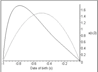
We now present some numerical illustrations of the impact of the initial wealth distribution on the capital dynamics. Let us consider the simplest possible case such that the economy begins at time τ = 0 and that the length of individual lifespan are normalized: ω = 1. Hence the initial dynamics cover the interval [0, 1] while the second dynamics hold for t ≥ 1. Moreover, assume that preferences are logarithmic (σ = 1) and that there is no time
discount (ρ = 0); the population is stationary (n = 0 and consequently β = 1) and there is no capital depreciation (δ = 0). Parameter of the production function have been chosen to be A = 100 and α = 0.01 such that the interest rate is normalized (r = αA = 1). In figure 1, we have plotted two initial distributions of wealth among generations at time τ = 0 that yield to the same initial aggregate capital per capita k (0) = 1. The solid line is the stationary distribution while the dashed line represents another initial distribution.
Figure 1: Initial wealth distribution.
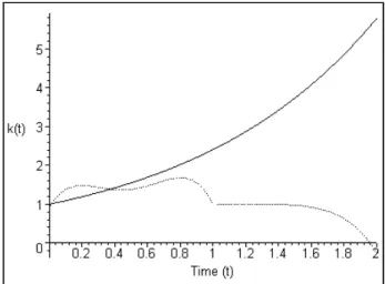
Using a procedure described in the Appendix, we have computed the dy-namics initiated by the two distributions. In Figure 2, we have plotted these dynamics. The solid line represents the behavior of the aggregate capital per capita when the growth rate is at its steady-state. The dynamics is hence exponential. The dashed line represents the solution of the dynamic system when the initial condition is the one given above. It first displays some echo effects around the balanced solution, but then fluctuations increase and the solution crosses the vertical axis. Such a path can therefore not constitute
an equilibrium path.
Figure 2. Aggregate dynamics.
4
Conclusion
In this paper, we have theoretically studied the intertemporal equilibrium path of an overlapping-generations model with finitely-lived individuals and constant returns to capital. We have shown that its existence lies on the ini-tial wealth distribution and that its dynamics to a balanced growth path is governed by exponentially decreasing oscillations. Such oscillations may be incompatible with the existence of an equilibrium. Economies with neoclas-sical production functions shall exhibit the same properties. Their dynamics are however characterized by a non linear MFDE which limit the theoreti-cal analysis to lotheoreti-cal dynamics and does not permit to solve analytitheoreti-cally the initial conditions problem. Applied to exchange economies, the method we have presented in this paper could also be used to study the issue of the in-determinacy of equilibrium path following the recent contributions of Kehoe et al. [16], Burke [8], and Ghiglino and Olszak-Duquenne [13].
Appendix
Proof of Lemma 1. The optimal consumption path satisfies for all t ≥ τ: ∂c (s, t) ∂t = σ [r (t)− ρ] c (s, t) , (38) and: Z s+ω t c (s, z) e−Utzr(u)dudz = a (s, t) + Z s+ω t w (z) e−Utzr(u)dudz. (39)
Equation (38) is the standard Euler condition while condition (39) is the intertemporal budget constraint obtained integrating forward condition (3) and using the optimal terminal conditions on assets:
a (s, s + ω) = 0 if ω ¿ +∞, limz→+∞e−Uszr(u)dua (s, s + z) = 0 if ω → +∞.
(40)
Using (38) and (39) allow to rewrite the optimal consumption such that:
c (s, t) = a (s, t) + Rs+ω t w (z) e− Uz t r(u)dudz Rs+ω t e− Uz t[(1−σ)r(u)+σρ]dudz . (41)
For individuals born at time s ∈ (τ − ω, τ) and still alive at time t ∈ (τ , τ + ω), the optimal consumption path is obtained using (41) to first define c (s, τ ); then with (38) one obtains:
c (s, t) = a (s, τ ) + Rs+ω τ w (z) e− Uz τ r(u)dudz Rs+ω τ e− Uz τ[(1−σ)r(u)+σρ]dudz eσUτt[r(u)−ρ]du, (42)
and then (6). Conversely, for individuals born at time s > τ , the initial consumption c (s, s) is obtained using the second equation of (4) and (41); then, with (38), one has:
c (s, t) = Rs+ω s w (z) e− Uz s r(u)dudz Rs+ω s e− Uz s[(1−σ)r(u)+σρ]dudz eσUst[r(u)−ρ]du, (43)
and then (7). ¤
Proof of Lemma 2. Replacing the assumption e (t) = k (t) in (22) and (23) yields factor prices: r (t) = αA − δ and w (t) = (1 − α) Ak (t). Moreover, at the equilibrium of the capital market, one has: a (t) = k (t). Hence (11) rewrites:
dk (t)
dt = [A− δ − n] k (t) − c (t) , (44) where c (t) is computed using (42), (43) and the factor prices to obtain:
c (t) = β Z τ t−ω a (s, τ ) e−n(t−s)eσ(αA−δ−τ)(t−τ) Rs+ω τ e−[(1−σ)(αA−δ)+σρ](z−τ)dz ds +β (1− α) A Z τ t−ω e−n(t−s)eσ(αA−δ−ρ)(t−τ)Rs+ω τ k (z) e−(αA−δ)(z−τ)dz Rs+ω τ e[(1−σ)(αA−δ)+σρ](t−z)dz ds +β (1− α) A Rt τ e[−n+σ(αA−δ−ρ)](t−s) Rs+ω s k (z) e−(αA−δ)(z−s)dzds Rω 0 e−[(1−σ)(αA−δ)+σρ]zdz ,(45) if t ∈ (τ, τ + ω) and: c (t) = β (1− α) A Rt t−ωe[−n+σ(αA−δ−ρ)](t−s) Rs+ω s k (z) e−(αA−δ)(z−s)dzds Rω 0 e−[(1−σ)(αA−δ)+σρ]zdz , (46) if t ≥ τ + ω. Let r = αA − δ, γ = n − σ (r − ρ) and µ = r − σ (r − ρ). Then, applying Fubini’s theorem and rearranging, (45) rewrites:
c (t) = z (t)− β (1 − α) Ae−nω Z t τ k (z) Z t z e−γ(t−s)e−r(z−s) Rs τ e−µ(u−s)du dsdz +β (1− α) Ae−σ(r−ρ)ωe−γ(t−τ) Z τ +ω τ k (z) Z τ +ω z e−γ(τ+ω−s)e−r(z−s) Rs τ e−µ(u−s)du dsdz −β (1− α) A Rt τ k (z) Rt z e−γ(t−s)e−r(z−s)dsdz Rω 0 e−µzdz −β (1− α) Ae −rωe−γ(t−τ)Rτ +ω τ k (z) Rτ +ω z e−γ(τ+ω−s)e−r(z−s)dsdz Rω 0 e−µzdz +β (1− α) Ae −rωRt+ω τ k (z) Rt+ω z e−γ(t+ω−s)e−r(z−s)dsdz Rω 0 e−µzdz , (47)
where z (t) is a function of time and initial conditions such that: z (t) = βe−γ(t−τ) Z τ t−ω a (s, τ ) e−n(τ−s) Rs+ω τ e−µ(z−τ)dz ds. (48)
Using (25) and (26) yields (30). Concerning (46), apply Fubini’s theorem and rearrange to obtain:
c (t) = −β (1− α) A ¡ 1 + e−(γ+r)ω¢ Rω 0 e−µzdz Z t τ k (z) µZ t z e−γ(t−s)e−r(z−s)ds ¶ dz +β (1− α) Ae −γω Rω 0 e−µzdz Z t−ω τ k (z) µZ t−ω z e−γ(t−ω−s)e−r(z−s)ds ¶ dz +β (1− α) Ae −rω Rω 0 e−µzdz Z t+ω τ k (z) µZ t+ω z e−γ(t+ω−s)e−r(z−s)ds ¶ dz.(49) Using (25) yields (31). ¤
Proof of Corollary 1. For ω → +∞, it is only equation (30) which is relevant for the dynamics. Remark with (9) that limω→+∞β = n if n > 0 and with (48) that limω→+∞z (t) = nµe−γ(t−τ)k (τ ) if µ > 0. Moreover, define
φ (ω) = e−nωv (t)˜ − e−σ(r−ρ)ωe−γ(t−τ)˜v (τ + ω)
−e−rωv (t + ω) + e−rωe−γ(t−τ)v (τ + ω) , (50)
where v (.) and ˜v (.) are respectively given by (25) and (26). Then compute limω→+∞φ (ω) = 0 to conclude. ¤
Proof of Lemma 3. For all t ≥ τ + ω, the dynamics of capital is given by (44) and (46). It will be useful to define the following variable:
x (t) = e−(αA−δ−n)tk (t) . (51) Then: dx (t) dt = (1− α) Ax (t) − β (1 − α) A Z t t−ω Rs+ω s x (z) eR −n(z−s)dz ω 0 e−µzdz e−µ(t−s)ds, (52)
where µ = (1 − σ) (αA − δ) + σρ. The characteristic equation Q (λ) is ob-tained by replacing x (t) by egt in (52). Hence:
Q (λ) = λ− (1 − α) A " 1− Rω 0 e−µs Rω 0 eλ(z−s)e−nzdzds Rω 0 e−nzdz Rω 0 e−µzdz # . (53)
At the exception of λ = 0, all roots of Q (λ) = 0 are relevant for the dynamics of x (t). Roots, denoted g, of the characteristic equation associated to the dynamics of k (t), denoted P (g), are then simply derived using g = λ + αA − δ− n. In what follows we characterize the roots of (53).
1) Real roots. Observe that Q (0) = 0, limλ→+∞Q (λ) = +∞ and:
Q00(λ) = (1− α) A Rω 0 e−µs Rω 0 (z− s) 2 eλ(z−s)e−nzdzds Rω 0 e−nzdz Rω 0 e−µzdz > 0. (54)
Hence, apart from λ = 0, there exists a unique real root denoted ¯λ. Moreover, since Q (n − µ) = n − µ, we have ¯λ < n − µ.
As a consequence, there exists a unique real root to P (g) denoted ¯g that satisfies ¯g < σ (αA− δ) − σρ.
2) Complex roots in the closed strip £min©0, ¯λª, max©0, ¯λª¤. Let λ = p + iq be a complex root of (53). We first prove there is no roots such that p ∈ ¡
min©0, ¯λª, max©0, ¯λª¢ by showing that Re (Q (p + iq)) < 0 in the open strip. Computation yields:
Re (Q (p + iq)) = p−(1 − α) A " 1− Rω 0 e−µs Rω 0Rep(z−s)cos (q (z− s)) e−nzdzds ω 0 e−nzdz Rω 0 e−µzdz # . (55) Then, we have Re (Q (p + iq)) ≤ Q (p) and we conclude using step 1 to state that Q (p) < 0 for any p ∈ ¡min©0, ¯λª, max©0, ¯λª¢. Consider now the complex root ¯λ + iq. If it were a root of (53), it would satisfy:
¯ λ− (1 − α) A " 1− Rω 0 e−µs Rω 0 e ¯ λ(z−s)cos (q (z− s)) e−nzdzds Rω 0 e−nzdz Rω 0 e−µzdz # = 0, (56)
This would imply that: (1− α) A ≤¯¯¯λ¯¯+(1 − α) A Rω 0 e−µs Rω 0 e ¯ λ(z−s)|cos (q (z − s))| e−nzdzds Rω 0 e−nzdz Rω 0 e−µzdz . (57)
Suppose |cos (q (z − s))| < 1 for some (z, s) ∈ [0, ω]2, then
(1− α) A <¯¯¯λ¯¯ + (1 − α) A Rω 0 e−µs Rω 0 e ¯ λ(z−s)e−nzdzds Rω 0 e−nzdz Rω 0 e−µzdz , (58)
which is not possible since Q¡¯λ¢ < 0. Suppose now |cos (q (z − s))| = 1 for all (z, s) ∈ [0, ω]2; it would imply q = 0. Apply the same procedure to show that the pure imaginary root iq is not a root of (53).
As a consequence, P (g) has no complex root with real part that belong to [min{αA − δ − n, ¯g} , max {αA − δ − n, ¯g}] except ¯g itself.
3) and 4) Complex roots of large modulus. They can be localized using the geometrical method proposed by Bellman and Cooke [4] p. 410. Their method is based on a distribution diagram. Compute equation (53) to obtain:
Q (λ) = λ− (1 − α) A " 1− nµ ¡ 1− e−(λ+µ)ω¢ ¡e(λ−n)ω− 1¢ (λ− n) (λ + µ) (1 − e−nω) (1− e−µω) # . (59)
Define ˜Q (λ) = (λ− n) (λ + γ) eλωQ (λ)such that:
˜ Q (λ) = λ (λ− n) (λ + µ) eλω− (1 − α) A (λ − n) (λ + µ) eλω + (1− α) Anµ ¡ eλω− e−γω¢ ¡e(λ−n)ω− 1¢ (1− e−nω) (1− e−µω) . (60)
Hence ˜Q (λ) is expressed asP3i=0P2j=0λiejλ. Then, plot the points xij with
6 -g3 g2 g eg e2g r r r r r r ££ ££ ££ £££BBB B B B B BB
Asymptotic roots are those of the convex envelop of the diagram. Here, the distribution diagram is composed of two segments L1 and L2 whose slopes
are respectively positive and negative. To L1 and L2 correspond two locus V1
and V2, which belong to C and where lie asymptotically the zeros of ˜Q (λ).
The zeros of L1 are those of function:
λ3eλω + (1− α) Anµe
−µω
(1− e−nω) (1− e−µω) = 0, (61)
which asymptotically have a negative real part. The zeros of L2 are those of
function:
λ3e−λω + (1− α) Anµe
−nω
(1− e−nω) (1− e−µω) = 0, (62)
which asymptotically have a positive real part. ¤
Proof of Corollary 2. On the balanced growth path, the capital growth rate, defined as (dk (t) /dt) /k (t), is constant. It is therefore given by the pure real root of the characteristic equation, namely ¯g. ¤
Proof of Corollary 3. Let λn ∈ C, be the roots of equation (53) and gn =
λn+ r− n, with r = αA − δ. Following Rustichini [20], define the following
subsets:
ΓS ={gn, Re(gn) < min{r − n, ¯g}} ,
ΓU ={gn, Re(gn) > max{r − n, ¯g}} ,
Now define MS (resp. MU, MC)the subset spanned by the roots that belong
to ΓS (resp. ΓU, ΓC). There exists three families of operators:
TS(t) : MS −→ MS for t > 0,
TU(t) : MU −→ MU for t < 0,
TC(t) : MC −→ MC for t ∈ (−∞, ∞) .
and there exists x > 0 such that for all φ ∈ MS, kTS(t)φk ≤ x kφk , for
all t > 0. Therefore elements of MS ∪ MC define the solutions kn(t) that
converge to the balanced growth path. To conclude on the dynamics of g (t) use the second point of Lemma 3, which demonstrate there is no cycle. ¤ Proof of Lemma 4. Equation (52) does not generate a semi group. However, we will consider it as an equation on the state space C [−ω, ω] , and in the following, we will consider kt(θ) = k (t + θ) for θ ∈ [−ω, ω]. Let us hence
first establish two preliminary results:
Claim 1. There exists µ > 0 such that κ (t) = e−µtk (t) solves an hyperbolic
differential equation of mixed type.
Proof of Claim 1. This is a direct consequence of the result established in the proof of Lemma 3 such that there is no complex roots in the closed strip [min{αA − δ − n, ¯g} , max {αA − δ − n, ¯g}]. ¤
Claim 2. Solutions that converge to the balanced growth path solve: dk (t)
dt = Z 0
−ω
k (t + θ) dη−(θ) , (63)
for t ≥ i + ω where dη−(θ) is a Lebegues-Stieljes measure on [−ω, 0].
Proof of Claim 2. According to Theorems 3.1 and 3.2 of Mallet-Paret and Verduyn Lunel [18], we have the direct sum decomposition C ([−ω, ω] , C) = P ⊕ Q, and we can define (as in the proof of Lemma 3) semi groups TQ(t)
and TP (−t) for all t ≥ 0. Applying then Theorems 5.1 and 5.3 we show that
these semi group can be represented, up to a finite mode, by delay differential equations. We will write the delay equation as:
dκ (t) dt =
Z 0
−ω
κ (t + θ) dη−(θ) . (64)
Then, use Claim 1 to obtain (63). ¤
Let A: D (A) → C ([−ω, 0]) be the generator of the semi group associated with (64). As in Diekman et al. [12] page 111, we give the explicit represen-tation of the resolvant of A. Let ζ = (zI − A)−1ϕ, where ϕ ∈ C [τ + ω, ∞). Then: zζ − ˙ζ = ϕ. Integrating this equation yields:
ζ (θ) = ezθζ (0) + Z 0
θ
ez(θ−s)ϕ (s) ds. (65)
Using the following boundary condition:
zζ (0)− Z 0 −ω ζ (s) dη−(s) = ϕ (0) , (66) equation (65) rewrites: zζ (0)− Z 0 −ω ezsζ (0) + Z 0 s
ez(s−u)ϕ (u) dudη−(s) = ϕ (0) , (67)
and thus: ∆−(z) ζ (0) = ϕ (0) + Z 0 −ω Z 0 s
ez(s−u)ϕ (u) dudη−(s) . (68)
Conclude that the resolvant of A has the following representation: ¡
(zI− A)−1ϕ¢(θ) = ezθ Ã
∆−1− (z) "
ϕ (0) +R−ω0 Rs0ez(s−u)ϕ (u) dudη −(s)
+Rθ0e−zsϕ (s) ds
#! . (69)
Then, since δn(λ) = resz=λ
¡
(zI− A)−1ϕ¢, one has:
δn(λ) = eλ. µ H (λ) ∙ ϕ (0) + Z 0 −ω Z 0 s
ez(s−u)ϕ (u) dudη−(s) ¸¶
, (70)
where H (λ) is defined by ∆ (z)−1 = H (z) / (z− λ) with H analytic at z = λ. ¤
Proof of Lemma 5. If τ → −∞, the dynamic system is given by equations (27), (29) and (31) only, which can be rewritten as an MFDE. Then, follow-ing Mallet-Paret [17], only pure real roots and pure imaginary roots of the characteristic equation are, if they exist, yield a solution which is bounded on R. Remark that the result can also be immediately derived from equation (36). ¤
Proof of Theorem 1. Consider the case such that ω and τ are finite. It has been shown in the proof of Lemmas 2 and 4 that the dynamics on the stable manifold writes as a functional equation with advances for t ∈ [τ, τ + ω] and with delays for t ≥ τ + ω. Let us consider the dynamics:
dk (t) dt =
Z t
t−ω
k (u) dη_ (t − u) for t ∈ [τ + ω, τ + 2ω] . (71)
If k (u) is given for u ∈ [τ, τ + ω], equation (71) is an ordinary differential equation which is non homogenous and linear. Let us denotes by ˆk (u), the path k (u) for u ∈ [τ, τ + ω]. Applying the constant variation formula, we can compute k (t) for t ∈ [τ + ω, τ + 2ω]. Let us denotes the solution as follows:
k (t) = ϕ³bk (u) ; u ∈ [τ, τ + ω]´. (72) The dynamics of k (t) for t ∈ [τ, τ + ω] is given by the differential equation (44) with (47) and (48). If k (u) is given for u ∈ [τ + ω, τ + 2ω], equation (44)
also becomes an ordinary differential equation which is non homogenous and linear. By simply applying the constant variation formula, we can compute k (t) for t ∈ [τ, τ + ω]. The solutions writes:
k (t) = φ (ϕ (k (u) , u∈ [τ, τ + ω]) , z (s) ; s ∈ [τ − ω, τ]) . (73)
where z (s) is a function of the initial wealth distribution given by (48). Differentiating (73) with respect to time yield to an ordinary differential equation that can be solved. The equation has an unique solution which depends on the initial condition.
We now illustrate this Theorem by computing the dynamics in a particular case. We will characterize the stationary distribution of wealth among gener-ation and the solution for any wealth distribution. To avoid tedious calculus, let us solve the dynamics in the simplest case such that τ = 0, ρ = 0, σ = 1, ω = 1, δ = 0 and n = 0 (and consequently β = 1). Define:
x (t) = k (t) e−αAt. (74)
Then, equation (44) rewrites: dx (t) dt = − Z 0 t−1 a (s, 0) (s + 1)ds + (1− α) A µ ln (t) Z t 0 x (z) dz− Z 1 t x (z) ln (z) dz ¶ − (1 − α) A µZ t 0 zx (z) dz− Z t+1 t x (z) (t− z + 1) dz ¶ , (75) for t ∈ [0, 1] and: dx (t) dt = (1− α) A µ x (t)− Z t t−1 (1− t + z) x (z) dz − Z t+1 t (1 + t− z) x (z) dz ¶ , (76) for t ≥ 1.
Let us first compute the steady-state distribution of wealth among the gen-erations. Differentiating (76) two times yields:
d3x (t) dt3 = (1− α) A ∙ d2x (t) dt2 + 2x (t)− x (t + 1) − x (t − 1) ¸ , (77)
for t ≥ 1 and let x (t) = x (1) e(¯g−αA)(t−1) where ¯g is the growth rate at
steady-state. Replace x (t) in (75), to obtain:
x (θ) = e(¯g−αA)(θ+1) "
(¯g− αA)2+ 2− e(¯g−αA)−(¯g− αA)
3 (1− α) A # , (78) for θ ∈ [0, 1] and : a (t− 1, 0) = tη£(¯g− αA)2+ (1− α) A (1 + t)¤e(¯g−αA)(t+1) −t (1 − α) Aη µZ t 0 e(¯g−αA)(z+1) t dz + Z 1 t e(¯g−αA)(z+1)dz ¶ −t (1 − α) A µZ t+1 1 e(¯g−αA)zdz ¶ , (79)
for t ∈ [0, 1] and with:
η = "
(¯g− αA)2+ 2− e(¯g−αA)− (¯g− αA)
3
(1− α) A #
. (80)
To characterize the dynamics, we use Lemma 5.7 of Mallet Parret and Ver-duyn Lunel [18] to compute the following equation:
dx (t) dt = (1− α) A x (t) 2 − (1 − α) A Z t t−1 x (z) (z− t + 1) dz + (1− α) A (λ − ¯g + αA) x (t) Z t t−1 (1− t + s) Z t s e(¯g−αA)(z−t)dzds − (1 − α) A (λ − ¯g + αA) Z t t−1 x (θ) Z θ t−1 Z θ s e(¯g−αA)(z−θ)dzdsdθ,(81)
whose roots of the characteristic equation are very close to the roots with negative real parts of (76). Remark that λ is the real root of the characteristic
equation of: x (t) = Z t t−1 (1− t + s) Z t s x (z) dzds. (82)
Then compute ϕ and φ as described in the first part of the proof. It is then possible to find an initial distribution such that k (t) < 0 on the interval [0, 2].¤
References
[1] H. d’Albis and E. Augeraud-Véron, Balanced cycles in an OLG model with a continuum of finitely-lived individuals, Econ. Theory 30 (2007), 181-186.
[2] H. d’Albis and E. Augeraud-Véron, Endogenous retirement and mone-tary cycles, forthcoming in Math. Population Stud.
[3] A. Auerbach and L. Kotlikoff, Dynamic Fiscal Policy, Cambridge Uni-versity Press, Cambridge, 1987.
[4] R. Bellman and K. Cooke, Differential Difference Equations, Academic Press, 1963.
[5] O. Blanchard, Debt, deficits and finite horizons, J. Polit. Economy 93 (1985), 223-247.
[6] R. Boucekkine, D. de la Croix and O. Licandro, Vintage human capi-tal, demographic trends and endogenous growth, J. Econ. Theory 104 (2002), 340-375.
[7] R. Boucekkine, O. Licandro, L. A. Puch and F. del Río, Vintage capital and the dynamics of the AK model, J. Econ. Theory 120 (2005), 39-72. [8] J. L. Burke, A benchmark for comparative dynamics and determinacy in overlapping-generation economies, J. Econ. Theory 52 (1990), 268-303. [9] J. L. Burke, Equilibrium for overlapping generations in continuous time,
J. Econ. Theory 70 (1996), 364-390.
[10] D. Cass and M. E. Yaari, Individual saving, aggregate capital accumu-lation, and efficient growth, in “Essays on the Theory of Optimal Eco-nomic Growth” (K. Shell, Eds.), pp. 233-268, MIT Press, Cambridge, MA, 1967.
[11] S. Demichelis and H. Polemarchakis, Frequency of trade and the de-terminacy of equilibrium paths: logarithmic economies of overlapping generations under certainty, Econ. Theory 32 (2007), 461-475.
[12] O. Diekmann, S. A. van Gils, S. M. Verduyn-Lunel and H. O. Walther, Delay Equations. Springer-Verlag, New York, 1995.
[13] C. Ghiglino and M. Olszak-Duquenne, On the impact of heterogeneity on indeterminacy, Int. Econ. Rev. 46 (2005), 171-188.
[14] H. J. Hupkes and S. M. Verduyn Lunel, Center manifold theory for functional differential equations of mixed type, J. of Dynamics and Dif-ferential Equations 19 (2007), 497-560.
[15] T. J. Kehoe, D. K. Levine, A. Mas-Colell and M. Woodford, Gross substitutability in large-square economies, J. Econ. Theory 54 (1991), 1-25.
[16] T. J. Kehoe, D. K. Levine, A. Mas-Colell and W. R. Zame, Determinacy of equilibrium in large-scale economies, J. Math. Econ. 18 (1989), 231-262.
[17] J. Mallet-Paret, The Fredholm alternative for functional differential equation of mixed type, J. of Dynamics and Differential Equations 11 (1999), 1-48.
[18] J. Mallet-Paret and S. M. Verduyn-Lunel, Exponential dichotomies and Wiener-Hopf factorizations for mixed-type functional differential equa-tions, forthcoming in J. of Differential Equations.
[19] J.-V. Rìos-Rull, Life-cycle economies and aggregate fluctuations, Rev. Econ. Stud. 63 (1996), 465-489.
[20] A. Rustichini, Functional differential equations of mixed type: the linear autonomous case, J. of Dynamics and Differential Equations 1 (1989), 121-143.
[21] G. Saint-Paul, Fiscal Policy in an Endogenous Growth Model, Quart. J. Econ. 107 (1992), 1243-1259.
[22] Ph. Weil, Overlapping families of infinitely-lived agents, J. Public Econ. 38 (1989), 183-198.