HAL Id: hal-02870294
https://hal.archives-ouvertes.fr/hal-02870294
Submitted on 16 Jun 2020
HAL is a multi-disciplinary open access
archive for the deposit and dissemination of
sci-entific research documents, whether they are
pub-lished or not. The documents may come from
teaching and research institutions in France or
abroad, or from public or private research centers.
L’archive ouverte pluridisciplinaire HAL, est
destinée au dépôt et à la diffusion de documents
scientifiques de niveau recherche, publiés ou non,
émanant des établissements d’enseignement et de
recherche français ou étrangers, des laboratoires
publics ou privés.
Smart Cities - The Optimization of their Development
Virgil Dumbrava, George Cristian Lazaroiu, Philippe Duquenne, Filip Carlea
To cite this version:
Virgil Dumbrava, George Cristian Lazaroiu, Philippe Duquenne, Filip Carlea. Smart Cities - The
Opti-mization of their Development. International Conference on ENERGY and ENVIRONMENT (CIEM),
Oct 2019, Timisoara, Romania. pp.162-166, �10.1109/CIEM46456.2019.8937594�. �hal-02870294�
OATAO is an open access repository that collects the work of Toulouse
researchers and makes it freely available over the web where possible
Any correspondence concerning this service should be sent
to the repository administrator:
tech-oatao@listes-diff.inp-toulouse.fr
This is an author’s version published in: http://oatao.univ-toulouse.fr/25257
To cite this version:
Dumbrava, Virgil and Lazaroiu, George Cristian and Duquenne, Philippe
and Carlea, Filip Smart Cities - The Optimization of their
Development. (2019) In: International Conference on ENERGY and
ENVIRONMENT (CIEM), 17 October 2019 - 18 October 2019 (Timisoara,
Romania).
Official URL :
https://doi.org/10.1109/CIEM46456.2019.8937594
Open Archive Toulouse Archive Ouverte
Smart Cities – The Optimization of their Development
Virgil Dumbrava and George
Cristian Lazaroiu
Department of Power Systems University POLITEHNICA of
Bucharest Bucharest, Romania v_dumbrava@yahoo.com
Philippe Duquenne
Industrial Engineering Department Institut National Polytechnique de
Toulouse Toulouse, France philippe.duquenne@ensiacet.fr
Filip Carlea
National Institute of Economic Researches 'Costin C. Kiritescu'
Romanian Academy Bucharest, Romania filip_carlea@yahoo.com
Abstract—The ongoing development and extensions of cities, as
well as the requirement for large scale deployment of renewable energy sources and electro-mobility determine the transformation of current electrical grids towards smart grids. The increasing demand and the requirement for its reliable supply is imposing new planning challenges for the development of electrical networks. The present paper describes a method of optimizing the development of urban electricity networks, by selecting from a set of available locations, the positions and the size of new power sources, using a multistage model. Results can be useful to plan the installation of new power sources in an existing network (distributed sources, renewable sources for powering electric vehicles).
Index Terms-- distribution network, multistage model,
optimization method, smart city.
I. INTRODUCTION
In agreement with current European Union framework plans for the development of exiting cities, the current electrical networks should evolve towards smart grids [1]. In addition, the requirement of pollutant reduction emissions within the cities is leading to a diversification of energy mix within city boundaries by large-scale integration of renewable energy sources. Also, the transportation sector is evolving and electro-mobility and storage systems large scale deployment is envisaged by 2030 and 2050. All this is requiring advanced information and telecommunication technologies with large data volumes to be managed and used [2].
The current operation of the electrical urban networks is done in a radial configuration. As nowadays the cities are evolving, with new residential districts being built new electrical networks configuration can be proposed [3-6]. The integration of electrical vehicle charging stations (slow/fast/ultrafast) and distributed storage systems impose further constraints in the design of future electrical networks. In addition, power quality and continuity of supply requirements are more and more restrictive for increasing the residents level of wellbeing satisfaction [7-10].
This paper proposes a model considering the existing and future potential power sources within the network. Hence, for an existing source, the unitary cost of energy supplied and the capacity of the source are known. For the new power sources, we will know the unitary cost of supplied energy, their capacities and a fixed cost needed for construction and procurement works. If a potential power source is out of operation, it cannot provide electricity and its fixed cost is no furtherly considered.
The remainder of the paper is organized as follows: the methodology with the optimization mathematical model (the objective functions and the constraints) is presented in section II. Section III reports the analyzed case study and the obtained results, while the conclusions are discussed in section IV.
II. METHODOLOGY The assumptions envisaged are as follows:
a) the maximum power that can circulate on each of the power lines of the network is known;
b) the cost of transporting electricity on a line is approximated by a linear function;
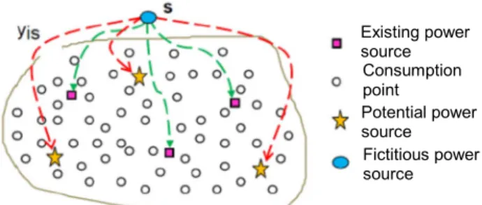
The studied electrical network is represented by a non-oriented connection graph with the source nodes (existing and potential) as well as the nodes corresponding to the consumers. The edges of the graph are determined by the power lines of the network. A fictive source vertex is introduced into the graph, which is considered a power supply for the entire power consumed in the network. Each vertex corresponding to an existing or potential source is connected by an edge to the fictitious point. Fig. 1 presents the modeled network with his main elements.
The following notations will be used:
s = fictitious source;
= 1, … , ∪ = set of source points;
J = {1, ..., n} = the set of the corresponding network
consumer points; This work was supported in part by a grant of the Romanian of Research and
Innovation, CCCDI – UEFISCDI, project number PN-III-P1-1.2-PCCDI-2017-0404/36PCCD/2018, within PNCDI.
Figure 1. Modeling of the studied network elements
N = I∪J = the set of graph’s vertices;
ai = the available power at the source i, i ∊N;
bj = power consumption at the consumer j, j∊N;
cij = cost of one kW transported from the source i to the consumer j, i ∊N, j∊N;
• cii = 0 ,∀i ∊N;
• cij = ∞ if the vertices i and j are not connected by an edge;
Pij = power absorbed from the source i by the consumer j, i ∊N, j∊N;
Dij= the maximum permissible power that can be carried on the line section i–j;
Fis = fixed cost associated with source operation at vertex i (Fis≠ 0 only for new sources);
yis =
0,
;
1,
.00
Using the above notations, the following mathematical model is written: + ∈ ∈ ∈ (1) , ∈ ∈ (2) = , ∈ ∈ (3) 0 , ∈ , ∈ , ≠ (4) 0 , ∈ (5) = 0 1 , ∈ (6) The equation (1) represent the objective function of the mathematical model, minimizing the total cost of the network development. The constraint (2) represents the condition that the sum of the power flows from source i to all the consumers must be inferior or equal to the power available at source i. The constraint (3) represents the condition that the sum of the power flows from all the sources to the consumer j must be equal to the power needed by the consumer j. The constraint (4) represents the condition that on each line section i-j, the power flow Pij must be inferior to the maximum permissible power on that line, Dij. The constraint (5) is similar to the constraint (4), but applicable only to the fictious lines is. The constraint (6) reflects the binary character of the yis variables.
The problem defined by the equations (1)–(6) has two types of variables, Pij and , which represents the optimization variables. For this reason, the problem is a mixed linear programming problem, having real continuous variables (Pij) as well as binary variables ( .
If each of the yis variables is set to either 0 or 1, the problem given by the equations (1)–(4) is a transport problem with limited capacities.
By enumerating all the situations in which the m binary variables yis can be found, a finite number of 2m transport
problems will result, by solving which can be determined the optimal solution of the problem (1)–(6).
This type of problem presented above was solved in [11] using the "branch and bound" method. But, starting from the fact that of the m variables yis only the ones corresponding to the potential sources can be interesting (by the fixed costs involved in commissioning) and considering the variables yis =1 for all the existing sources in the network, another solution will be proposed in this paper for the problem (1)–(6) using the "backtracking" method.
We will use the notations:
I '= the set of potential source vertices,
I '⊆I, card I' = m'≤ m; (7)
Y '= vector containing the m' variables yis, i∈I '. (8) Under these circumstances, from the 2m distinct problems in
which the problem (1)–(6) can be decomposed, we will only be interested by 2m' problems. In addition, by applying the
backtracking method, it will not be necessary to research all of the 2m' possible solutions.
Thus, elements of the vector Y' are assigned values one by one. For the variable is given a value of 0 or 1 only if values Existing power source Consumption point Potential power source Fictitious power source
for the variables , … , , have already been assigned. After setting a value for the variable , the algorithm does not go directly to the assignment of values to , but verify first a continuity condition for , … , . This condition determines the situations in which it makes sense to pass to the calculation of , failure to do so by expressing the fact that if we choose , … , , anyway, we cannot reach a possible solution to the problem (1)–(6). If the continuation condition is not met, another choice will be made for or, if this is not possible, k is reduced by one unit and a new value for the current variable is attempted.
If we denote with PT the total power demanded by the consumers in the grid, with the PE power provided by the existing sources and with PP the proposed power to be installed in the new sources, we will have:
PP ≥ PT - PE (9)
Thus, we can consider as continuation condition for the backtracking algorithm to solve the problem (1)–(6) reduced according to the notations (7) and (8), the requirement that the sum of the available power in the potential sources for which the corresponding ys variables do not have yet the value 0 (these sources can still be put into operation) be at least equal to the PP value. By denoting with I" the subset of I formed from potential sources for which the variables yis were given the value 0, the continuation condition can be written as:
≥
∈ \" (10)
The condition (10) assure us that it is still possible to obtain a possible solution for the problem (1)-(6), considering all the values granted so far for the variables yis.
For each of the final vectors Y' obtained by respecting condition (10), the condition (10) for validation of the value of the last variable is checked again, after which a transport problem (1)–(5) with fixed yis values is solved. Among the solutions to these problems will finally be selected the optimal solution or, in other words, the sites in which new power supplies will be put into operation.
III. CASE STUDY
Let us consider a network having 20 consumption points, from which 3 power supplies (1, 2 and 3) already exist and 3 locations are proposed to install new sources (4, 5 and 6). The values PT = 2100 kVA, PE = 1200 kVA, PP = 900 kVA are known. Table I reports the capacities and fixed costs for each of the m = 6 power supplies.
For this example, we will have thus: • m = 6 and m' = 3;
• I = {1,2,3,4,5,6} and I'= {4,5,6};
• (Y')t= (y4s, y5s, y6s).
In Table I are presented the capacities of existing power sources (1, 2 and 3), the capacities that can be installed in the new potential power sources (4,5 and 6), as well as the fix costs (given in monetary units, only for the new power sources).
TABLE I. INSTALLED POWER AND FIXED COSTS ASSOCIATED WITH SOURCES
Source no. Sn(kVA) Fixed Cost (m.u.)
1 400 0 2 400 0 3 400 0 4 250 4000 5 650 4500 6 400 3500
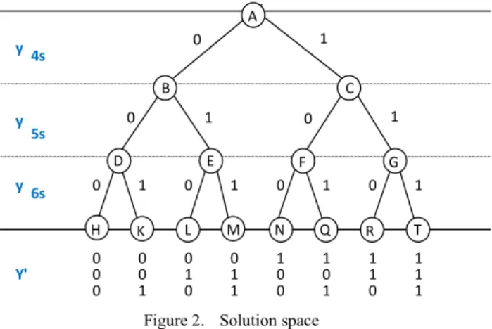
There are therefore 2m'= 23 = 8 possibilities of operation for
the new 3 potential sources. The mode of determination, according to the backtracking method, of the 2m'vectors Y' is
illustrated in Fig. 2, where the solution space was represented for the studied example.
B A C D E F G H K L M N Q R T 0 1 0 1 0 1 0 1 0 1 0 1 0 1 y y y 4s 5s 6s Y' 0 0 1 1 0 0 1 1 0 1 0 1 0 1 0 1 0 0 0 0 1 1 1 1
Figure 2. Solution space
The search of the solutions starts from the vertex A. By giving to the binary variable y4s the value 0 (the first possible value) we reached the vertex B of the binary tree which describes the generation process of all eight vectors Y'. Being in B, we verify the fulfillment of the continuation condition (10):
" = 4 ; = + = 650 + 400 = 1050
∈ \"
> = 900 ; = 0, , .
The value 0 is then assigned to the variable y5s , reaching the D vertex. From verification of the continuation condition, it follows that a possible solution cannot be obtained if y4s and y5s are equal to zero:
" = 4; 5 ; = = 400 = 400 < ∈ \"
= 900 ; = 0, 0, .
Therefore, it is not necessary to examine the vertices H and K, but returns to the vertex B, giving to the binary variable y5s the other remaining available value, the value 1, thus reaching the vertex E. The continuation condition is also checked here:
" = 4 ; = + = 650 + 400 = 1050
∈ \"
> = 900 ; = 0, 1, .
Next, we assign a value to the variable y6s . Fixing y6s = 0, we reached the vertex L. The solution obtained cannot be accepted because it does not fulfill the condition (10):
" = 4; 6 ; = = 650 = 650 <
∈ \"
= 900 ; = 0, 1, 0 .
Consequently, we return to the vertex E and we assign the next available value to the binary variable y6s , that is, the value 1, thus arriving to the vertex M. The new solution corresponding to the vertex M fulfills the condition (10):
" = 4 ; = + = 650 + 400 = 1050
∈ \"
> = 900 ; = 0, 1, 1 .
Y'M is the first possible solution obtained until now. For the
determination of other solutions, since the variables y6s and y5s have taken all their possible values, we return to the vertex A and we assign to the binary variable y4s the next available value (that is 1), thus moving to the vertex C. We must verify here also the condition of continuation:
" = 0 ; = + + = 250 + 650 + 400
∈ \"
= 1300 > = 900 ;
= 0, , .
We continue the displacement in the solution space, and we assign then the value 0 to the binary variable y5s, reaching so the vertex F. The continuation condition is not met at the vertex F:
" = 5 ; = + = 250 + 400 = 650
∈ \"
< = 900 ; = 1, 0, .
By not respecting the continuity condition at the vertex F, the final solutions corresponding to the N and Q vertices will not be further investigated. Returning to the vertex C, we will assign the next available value to the binary variable y5s, that is the value 1. At the vertex G, the continuation condition is met:
" = ∅ ; = + + = 250 + 650 + 400
∈ \"
= 1300 > = 900 ; = 1, 1, .
If the variable y6s is then assigned to 0, the final solution at the vertex R will satisfy the condition (10) and therefore R will represent another possible solution, the second one:
" = 6 ; = + = 250 + 650 = 900
∈ \"
= = 900 ; = 0, 1, 1 .
The last solution is obtained by returning to the vertex G and fixing the variable y6s to the value 1. The final solution, corresponding to the vertex T, met the condition (10):
" = ∅ ; = + + = 250 + 650 + 400
∈ \"
= 1300 > = 900 ; = 1, 1, 1 .
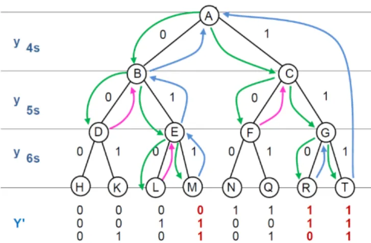
Fig. 3 presents the trajectory of the algorithm through the solution space. Green lines represent movements in the depth of the solution space, red lines represent returns due to non-fulfillment of condition (10), while blue lines represent returns to the next possible value for the current binary variable.
Figure 3. Trajectory of the algorithm in the solution space
Therefore, from the 2m '= 23 = 8 possibilities to install the
new power supplies, only 3 represents possible solutions, namely Y'M, Y'R and Y'T. To further determine the locations in
which new power supplies will be deployed, we will now solve 3 transportation problems with the y4s, y5s and y6s variables fixed according to the three possible solutions above (M, R and T). From the three possible locations of the new sources, it will be chosen the one having the lowest value of the objective function (1).
The efficiency of the backtracking method presented is given by the ratio between the number of transport problems solved by its application, NBM, and the number of transport
problems required to be solved by the enumeration method, NT.
It must be said that the enumeration method will identify, for the analyzed example, 8 solutions, for all this, then a transport problem must be solved. This ratio (NBM/NT) will show how
many of the total number of solutions has been studied to get the best solution of the problem. So,
∙ 100 =3
8∙ 100 = 37,50%
As a result, the analysis of 62.5% of the solutions were avoided for the studied example. The percentage of efficiency depends on the size of the problem (the number of potential sites) and on the power to be installed in the network and on the power installed at each site.
If ai ≥ PP, ∀ i ∈ I', so if the power available in each potential new site is at least equal to the total power required to be installed in the grid, 2m’-1 possibilities of operation of the new
sources will have to be investigated. The amount of power available in each potential site is not determined in this method.
If the variables yis are also left free for the existing sources in the network and if the available power of the new potential sources is large enough, solutions can be found where some of the existing sources are closed (due to the losses of energy they generate though the electrical lines of the grid), their consumers being supplied more economically by the rest of existing sources along with new ones.
By solving transport problems, the topology of the electrical network's operation schemes will be mixed, with both dual-source and radial-fed consumers.
The constraint (4) corresponds to the requirement to limit the power flow through the network lines to the maximum allowable values Dij. For the optimal solution, however, the level of voltages in the nodes of the network must be checked, as there is no such verification in the method presented.
IV. CONCLUSIONS
The present paper describes a method of optimizing the development of urban electricity networks, by selecting from a set of available locations, the positions and the size of new power sources, using a multistage model. As results, we obtain the optimum number of sources and their size, as well as the topology of the new electrical lines. The optimization model assures also the minimization of the operation costs of the network (mainly the cost losses of energy in the electrical lines), including the costs for the new sources.
REFERENCES
[1] The European Innovation Partnership on Smart Cities and Communities (2017). http://ec.europa.eu/eip/smartcities/. Accessed 10 March 2019 [2] V. Dumbrava, Th. Miclescu, G.C. Lazaroiu, "Power distribution
networks planning optimization in smart cities", in City Networks:
Collaboration And Planning For Health And Sustainability,vol. 128 Ed.
Sprin, 2017, pp. 213-226.
[3] G. C. Lazaroiu, V. Dumbrava, M. Costoiu, M. Teliceanu and M. Roscia, "Energy-informatic-centric smart campus", Proc. 2016 IEEE 16th
International Conference on Environment and Electrical Engineering (EEEIC), Florence, Italy, 2016, pp. 1-5.
[4] G. C. Lazaroiu, V. Dumbrava, M. Costoiu, M. Teliceanu and M. Roscia, "Smart campus-an energy integrated approach", Proc. 2015
International Conference on Renewable Energy Research and Applications (ICRERA), Palermo, Italy, 2015, pp. 1497-1501.
[5] G. Celli, F. Pilo, G. Pisano, V. Allegranza, R. Cicoria and A. Iaria, "Meshed vs. radial MV distribution network in presence of large amount of DG," IEEE PES Power Systems Conference and Exposition, 2004., New York, NY, 2004, pp. 709-714 vol.2.
[6] V. Dumbrava, C. Lazaroiu, C. Roscia and D. Zaninelli, "Expansion planning and reliability evaluation of distribution networks by heuristic algorithms", Proc. 2011 - 10th International Conference on Environment
and Electrical Engineering (EEEIC), Rome, Italy, 2011, pp. 1-4.
[7] I. Sharma, C. Cañizares and K. Bhattacharya, "Smart Charging of PEVs Penetrating Into Residential Distribution Systems", in IEEE
Transactions on Smart Grid, vol. 5, no. 3, pp. 1196-1209, May 2014.
[8] P. S. Georgilakis and N. D. Hatziargyriou, "Optimal Distributed Generation Placement in Power Distribution Networks: Models, Methods, and Future Research", in IEEE Transactions on Power
Systems, vol. 28, no. 3, pp. 3420-3428, Aug. 2013.
[9] S. Haffner, L. F. A. Pereira, L. A. Pereira and L. S. Barreto, "Multistage Model for Distribution Expansion Planning With Distributed Generation—Part I: Problem Formulation", in IEEE Transactions on
Power Delivery, vol. 23, no. 2, pp. 915-923, April 2008
[10] S. Haffner, L. F. A. Pereira, L. A. Pereira and L. S. Barreto, "Multistage Model for Distribution Expansion Planning with Distributed Generation—Part II: Numerical Results", in IEEE Transactions on
Power Delivery, vol. 23, no. 2, pp. 924-929, April 2008
[11] G.L. Thompson, D.I. Wall, “A branch and bound model for choosing optimal substation locations”, in IEEE Transactions on Power