Characterizing Surface Roughness From Pressure-Joint Closure Measurements Using Inversion Procedure

PRESSURE-JOINT CLOSURE MEASUREMENTS

USING INVERSION PROCEDURE

by

Xiaomin Zhao and M. Nafi Toksoz Earth Resources Laboratory

Department of Earth, Atmospheric, and Planetary Sciences Massachusetts Institute of Technology

Cambridge, MA 02139

ABSTRACT

An inversion procedure has been formulated to estimate the surface roughness of a joint (fracture) from the measured pressure-closure data. A gamma distribution for the local minima (or maxima) on a topography profile was used to account for the skewness in the measured distribution of the asperities. By using the distribution, the average height

z

and the standard deviation a of the profile can also be characterized. An inversion procedure was formulated based on the modification of the theory proposed by Brown and Scholz (1985) and has been successfully tested with synthetic data. The inversion finds average height

z,

standard deviation a, and average aperture. These three parameters characterize the surface roughness and aperture of a fracture and are the topography parameters governing permeability, electric conductivity and other transport properties of the fracture. Pressure-closure data from laboratory measurement of a rough and a smooth joint were also inverted to find the joint properties. The results agree with the profile measurement qnite well. The variations of transport properties of a fracture with pressure are also studied.

INTRODUCTION

The physical contact between two rough surfaces is referred to as a "joint". The closure of such a joint under normal stress (or pressure) depends not only on the elastic con-stants of the material but also on the details of the surface topography (or roughness). Considerable work has been done to investigate the behavior of cracks under pressure (Kuster and Toksoz, 1974; Toksoz et al., 1976; Cheng and Toksoz, 1979; Gangi, 1978, 1981; Walsh and Grosenbaugh, 1979; Batzle et aI., 1980; Tsang and Witherspoon, 1981; Walsh and Brace, 1984; Carlson and Gangi, 1985; Brown and Scholz, 1985, 1986; Wong et aI., 1989; Yoshioka and Scholz, 1989a,b).

154 Zhao and Toksoz

(

Gangi (1978) has used a "bed of nails" model for a fracture joint to determine the stress dependence of closure of a fracture and permeability in fractured rock. Tsang and Witherspoon (1981) have described the closure of fracture as resulting from the deformation of "voids" or "cracks" between asperities and predicted the elastic prop-erty of rocks. Brown and Scholz (1985, 1986) have measured the surface topography of ground glass and rock surfaces and used it in connection with the elastic contact theory following from Greenwood and Williamson (1966) to explain the observed data of pressure-joint closure measurements.

Inthese studies, the primary concern was in the modeling of the pressuclosure re-lation using the surface roughness properties, although some researchers have estimated the surface roughness parameters by fitting experimental data using the forward models (Gangi, 1978; Carlson and Gangi, 1985; Brown and Scholz, 1985). It would be useful to construct a formal inversion procedure to determine the crack surface topography, which is the major interest of this study. We use the modified version of the theory of Brown and Scholz (1985) for forward modeling. Our modification properly accounts for initial aperture, and uses a gamma distribution function (Yoshioka and Scholz, 1989a,b) for local maxima (sunnnits of asperities). For the inverse problem, the inversion pro-cedure is tested using synthetic pressure-closure ( P ~8) data to invert for the model parameters

z,

0', and

(z-do),

where

z

is the average height,0' is the standard deviation,

and (z - do) is the initial aperture. These three parameters can be used to assess the roughness of the surface and the aperture between the two surfaces. More important, the inverted parameters, together with the forward model, can be used to predict the change of transport properties (such as permeability and electric conductivity of the fracture) with pressure. Therefore, the method described in this study provides a useful technique for the study of joint properties.

FORWARD PROBLEM

Brown and Scholz (1985) generalized Greenwood and Williamson's (1966) theory of normal elastic contact of two surfaces (one rough and one flat) and derived an expression for normal contact between the two rough surfaces. First, they defined the concept of composite topography z

=

Zl

+

Z2, where Zl and Z2 are the heights of each surface

measured from their respective reference planes (see Figure 1 of Brown and Scholz, 1985). Based on the composite topography, the relation between the normal stress P and joint closure 8 can be written as:

( 4 1

1

00 3 P(8)

=

-31]

<

'ljJ

><

E'

><

1<.'

>

(z - d

+

8)'q,(z)dz

d-o

(1)

where: z TJ

<1/1>

<

E'

>

1

<

I<~

>

¢(z) d {j P

height of local maximum on the composite topography; total number of local maxima per unit area;

mean value of tangential stress correction factor; mean value of elastic constant;

mean value of square root of curvature term;

probability density distribution for the local maxima; distance between the two reference planes at P

=

O. amount of closure

normal pressure

The probability density function ¢(z) is the probability that a local maximum (or min-imum) on the composite topography will have a height between z and z

+

dz. Initially, Gaussian distribution was commonly adopted (Nayak, 1971, 1973a,b) for the surface height. However, actual measurements showed that distribution is skewed towards pos-itive heights and an inverted X2 distribution for the surface heights was found to be a better model (Adier and Firman, 1981). From the distribution of the surface heights (any point on the topography), a complicated expression for the height of local maxima was derived (see Adler and Firman, 1981, Eq. 6.9) and was used as ¢(z) in Eq. (1) by Brown and Scholz (1985). A more generalized form of the X2 distribution, I.e., the gamma distribution, was proposed by Yoshioka and Scholz (1989a,b):

z'"

( z)

¢(z) = r(a

+

1).6"'+1 exp

-73

.

(2)

Since a measured local maxima (or minima) distribution that has skewness can be well fit using this simple distribution function by adjusting the values ofaand (3, we adopted the gamma distribution for ¢(z) in the present work. The mean height

z

and standard deviation (j of the gamma distribution are

{

z

(j2

-

=

(a

+

1)(3

z(3 . (3)

The choice of z in this study is in reverse direction of the z axis of the composite topography of Brown and Scholz (1985), as illustrated in Figure 1. Thus their maxima become minima on the composite topography in this study. When the distribution (Eq. 2) is used for the minima on the composite topography, the parameter

z

measures the average height of the asperities, and (j, the deviation of the asperities from this

mean height. Generally, a rough surface is characterized by large values of

z

and (j,

while a smooth surface by small values of

z

and(j. Therefore, by estimating a and (3 of

156 Zhao and Toksoz

InEq. (1), however, there are two imprecise parameters. One is the collective term that pre-multiplies the integral, M

=

'7

< !/J ><

E'

><

d

>.

The other is d, the distance between the two reference planes at zero pressure. The termM involves several surface topography and material property parameters that are not easily measurable (Brown and Scholz, 1985). We set this collective term as a parameter that is to be inverted. The d value is also somewhat uncertain. With the choice of z in Figure 1, this parameter is redefined. We also use do to distinguish it from parameter d in Eq. (1). When the two surfaces are placed together, there are a number of points that are in contact. Ifwe take the reference plane that contains the contacting points (i.e., the highest points in Figure 1) as the z = 0 plane, Eqn (2) then indicates that the probability for these points to exist is zero (¢(O) = 0), contrary to the fact that these contacting points do exist. Therefore, the reference plane must be set at z

=

do, at which the probability for the contacting points on the composite topography is ¢(do).

This configuration is also shown in Figure 1. Physically, we may think of do as the initial overlap of the two surfaces when they are placed together before the application of normal stress P. For the configuration of Figure 1, Eq. (1) is modified to become:

(

(4) The physical meaning of Eq. (4) can be explained. When a closure 8 is produced by a normal stress, the z

=

do plane is displaced to the z

=

do

+

8 plane. The asperities that exist between z and z

+

dz are ¢(z)dz and their distortion due to 8 is (do

+

8 - z) For spherical asperities, the contacting stress generated is proportional to the distortion to the power of 3/2 (Timoshenko and Goodier, 1951). Summing the contributions over the interval [do, do

+

81

and multiplying by M gives the total normal stress applied on the joint. Therefore, for a given topography, which is characterized by a,

fl,

and do, and a given material, the relationship between the normal stress P and the resulting joint closure 8 can be modeled by Eq. (4). We point out that, since 8 is generally small, Eq. (4) or Eq. (1) uses only a small fraction of¢(z), (see Figure 1), so that any distribution function [e.g. power law (Gangi, 1978); Gaussion and X2 functions (Brown and Scholz, 1985)J that has the similar behavior in the small interval [do, do

+

8J will achieve essentially the same results.

INVERSE PROBLEM

Based on the forward model given in Eq. (4), an inverse problem can be formulated to estimate M, a,

fl,

anddo from the measured P versus 8 data. Sensitivity analysis shows that the model is most sensitive to a and

fl,

and least sensitive to the multipierM. This indicates that the surface topography plays the most important part in determining the shape of the measured P ~ 8 curves.

The inversion consists of the minimization of two sources of errors: (1) the misfit between the predicted value of P from the model and the measured P at each given closure 8, and (2) the misfit between the estimated model parameters and the initial guesses. In terms of these two errors, the cost function <I>(m) is constructed as

where mT

=

_[M,a,)3,do], and T denotes transpose. The data covariance matrix CD

contains the error estimate of each data point. The matrix is diagonal because all data measurements are assumed to be independent. The model covariance matrix, also diagonal because of the independence of model parameters, can be estimated by the possible range of variation of each model parameter. The cost function is minimized with respect to m to find the best choice ofM, a, )3, and do. The minimization uses a Levenberg-Marguardt algorithm which has been developed for nonlinear, least-squares problems (More, 1978).

RESULTS AND DISCUSSION

Synthetic Example

We test the inversion procedure using synthetic P ~ 8 data calculated with Eq. (4) with

M = 100 MPa, a = 10, )3= 311m, and

do

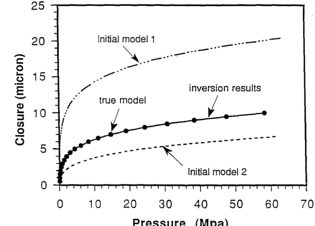
= 1011m. Different initial models were chosen as the input of the inversion program and the P ~ 8 curves of all the inversion results converge to the synthetic P ~ 8 curve. The inverted model parameters from different initial models are in close agreement with the true model values. Especially, in terms of the average height

z,

the standard deviation (5, and the aperture without pressure (z - do), the inverted results agree with the true values very well. As an example, two sets of the inversion results are plotted in Figures 2 and 3. The two different models are

M = 80 MPa, do = 811m, a = 8, and)3= 2.5 11m, (initial model 1), and M = 150 MPa,

do

= 15 11m, a = 12, and )3 = 5 11m, (initial model 2), respectively. Figure 2 shows the inversion

P

~ 8 curves of the two different initial models. Figure 3 compares the inverted topography parameters

(z,

(5, and

z -

do)

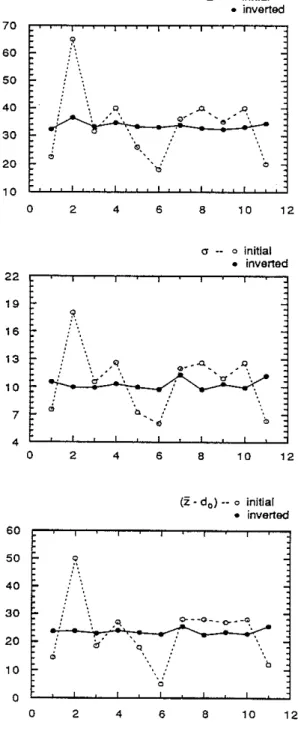
from the two initial models with the true model parameters. Some more examples are shown in Figure 4, in which the inversion results from ten different initial models are plotted together with the initial model parameters. The inverted parameters from the ten different initial models are quite close, and are in good agreement with the true model parameters, considering the fact that their initial guesses are significantly different (see Table 1 for detail). In fact, the forward model given in Eq. (4) is governed mainly by the integral. For a given 8, the value of predicted pressure P depends on the area covered by the integrand in the interval [do, do

+

8]. This area is largely dependent on the probability density ¢(z), and therefore

z,

and (5. The average height

z

measures how far away the center of¢(z) is

158 Zhao and Toksoz

from the z

=

0 plane, and a, the flatness of ¢>(z). The inversion tries to find a ¢>(z)

(governed byz and a) that gives the area in [do,

do

+

8J that is required to match the givenP ~8 data. Therefore,

z

and a are more explanatory of the results. The quantity (z - do) is a measure of the average initial distance between the two surfaces, which is an important parameter for the joint transport properties such as permeability and electric conductivity (Brown, 1987,1989). The excellent agreement between the inverted

z,

a

and ("2 -

do)

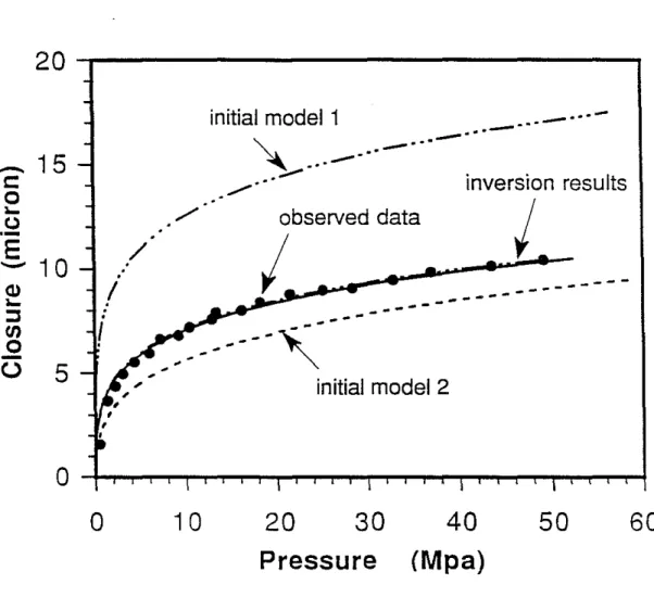
and those of the true model gives us confidence in the inversion procedure for the problem.

Inversion of Laboratory Experimental Data

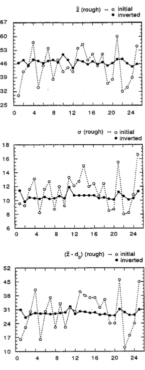
(1) Rough Surface

One set of the laboratory data of Brown and Scholz (1986) was used for the inversion. The invertedP ~ 8 curves from 25 different initial models converge to the observed data quite well. As an example, Figure 5 gives the observed and the inverted P ~ 8 curves from two quite different initial models. Similar to the inversion results of the synthetic data, although an inverted individual parameter such as do (or a, or ;3) from different initial models may not be exactly the same, the surface topography parameters"2 and a calculated from different models are quite close to each other (see Figure 6). Infact, we got"2

=

46.92

±

1.44J.lm, a

=

10.56

±

0.46J.lm, and ("2 - do)

=

29.28

±

1.18J.lm, for this profile. The smaller variations of the inverted"2and a indicate that these parameters are relatively well estimated. This result is useful since

z

and

a

characterize the surface topography better thana and ;3.

Table 2 compares the average and deviation of the inverted (z -

do)

and a values from the 25 different initial models with the profile measurement results of Brown and Scholz (1986). Note that in Brown and Scholz (1986), d is measured from the mean of the distribution of composite topography (Gaussian or inverted X2) to the highest

point(s) of the topography. Thus their d value is analogous to ("2 - do) in this study. However, if measured from

z

=

0, the mean of the asperities ("2) should be smaller than the mean of the topography (i.e., all heights) (see Figure 5 of Brown and Scholz, 1985). Therefore, our (z - do) should be slightly less than their d value (do in their original paper). The measured d value in their paper ranges from 23 to 40 J.lm (best fitting value 33.3 J.lm) for this particular sample, and our inverted ("2 - do) based on 25 different initial models is 29.28

±

1.18 J.lm, The two values are in good agreement. In addition, the inverted standard deviation is 10.56

±

0.5 J.lm, agreeing with the measured value 12.9 J.lm. These large values of z (or "2 - do) and a are in agreement with the fact that these surfaces are rough surfaces. As we will see in the next example, smooth surfaces have smaller

z

and a values.

(

(

(

(2) Smooth Surface

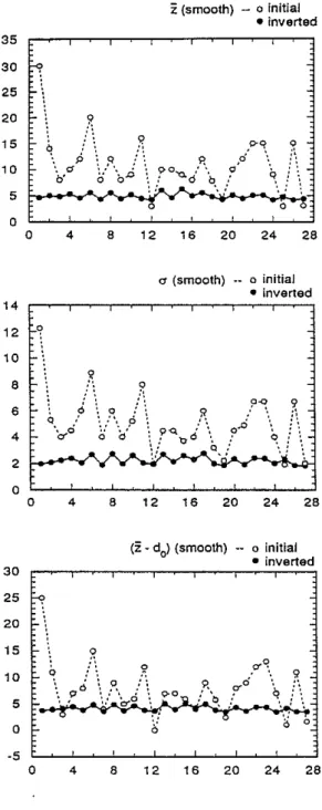
The experimental P ~6 data of Yoshioka and Scholz (1989), measured using a smooth joint, were used for the inversion. Figure 7 shows the good fit of the inverted P ~ 6 curves from two different initial models with the observed data. Figure 8 shows the inverted parameters Z, (J", and (21 - do) from 27 different initial models. Again, as the inversion results of the synthetic and the experimental data of a rough surface, the 21, (J", and (21 - do) values calculated from the inversion parameters are quite close. As expected from the physical intuition, the smooth surface has smaller values of21, (J", and (21 -

do).

For this example, we obtain21 "" 4.89

±

0.56 j1.m, (J" "" 2.22

±

0.30 j1.m, and (21 - do) "" 4.12

±

0.52 j1.m from the 27 different initial models. For comparison with experimental results, we measured the 21 value from the observed topography data of Yoshioka and Scholz (1989a, Figure 5, 1989b, Figure 4). This gives21 ""4.5j1.m. The (J" value was calculated by using ¢(z

+

(J") "" 0.7¢(z) according to statistical theory. The estimate is (J" ""'2.0j1.m. The comparison is also given in Table 2. The inversion results agree well with the experimental results.

APPLICATION TO JOINT TRANSPORT PROPERTIES

The results of this study can be used to study the transport properties of joint fracture. The variation of the flow properties with pressure is of importance in hydrology and petroleum production in fractured reservoirs. This variation can be predicted with the results of this study.

The transport properties are primarily controlled by the effective aperture of the fracture joint (Brown, 1987). The inversion results of this study give an estimate of

(21 - do), which is a measure of the aperture between the rough surfaces in the absence of the pressure. As the pressure is applied, a closure 6 is produced and the effective aperture becomes(21 - do - 6). The volumetric fluid flow rate through a fracture of unit length is proportional to (21 - do - 6)3 (the cubic law, Snow, 1965), the electric current conducted by the fracture is proportional to(21 - do - 6) (Brown, 1987). Since theP ~6 relation is given by Eq. 4 for the inverted parameters M, do, 21, and (J", the transport properties as a function of pressure can be predicted. Figure 9 gives the volumetric flow rate as a function of pressure. The two quantities are normalized with respect to their zero-pressure values. This figure is calculated using the inverted parameters for both rough and smooth joints, as indicated in Figure 9. Gangi (1978) also calculated the total permeability of a joint across a cylinder versus pressure using his "bed of nails" model (see Figure 7 of Gangi, 1978). Comparing Figure 9 with his results, we see the variation sof permeability with pressure of our model and Gangi's (1978) model are very similar. That is, they all have infinite slopes but finite values at P

=

0 (MPa), and decrease drastically as pressure increases.

160 Zhao and Toksoz

CONCLUSIONS

An inversion procedure has been formulated to estimate the surface roughness of a fracture from pressure-closure measurement data. A modified topography distribution model of Brown and Scholz (1985) was used to properly describe the rough surface and was used in the inversion process. The major features of this modified model are: it has a simplier distribution function (I.e., the gamma distribution) in our coordinate system; it characterizes the skewness of the measured distribution of the asperities by two parameters of the distribution function which can be inverted from the observed pressure-closure data; and it properly accounts for the initial aperture. The inversion results of synthetic pressure-closure data show good agreement of the inverted model parameters with those of the true model. The pressure-closure curves calculated using the inversion results converge to the synthetic calculated curve very well. The results inverted from laboratory measured data for both rough and smooth surfaces are quite reasonable and agree with the experimental measurements.

The transport properties of a fracture are functions of aperture and can therefore vary with the pressure applied on the joint. With the parameters inverted from the pressure-closure data, the forward model of this study was used to predict the change of the transport properties with pressure. The results are in good agreement with Gangi's (1978). Therefore, the results of this study can be used to study the change of transport properties (such as the permeability and electric conductivity) with pressure.

ACKNOWLEDGEMENTS

We thank Prof. B. Evans and R. Gibson for their helpful discussions and suggestions. This research was supported by Department of Energy Grant #DE-FG02-86ER13636 and the Full Waveform Acoustic Logging Consortium at M.LT.

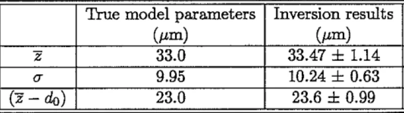
Table 1. Comparison of inverted model parameters with true model parameters of the synthetic data

True model parameters Inversion results

(pm) (/Lm)

z 33.0 33.47

±

1.14

(J" 9.95 10.24

±

0.63

(z - do) 23.0 23.6

±

0.99

Table 2. Comparison of inverted model parameters with experimental measurement data

Z (/Lm) (J" (/Lm) z - do (/Lm)

Estimated Inverted Estimated Inverted Estimated Inverted from profile results from profile results from profile results

Rough

-

46.9

±

1.4 12.9 10.6

±

0.5 23 - 40 29.3

±

1.2

162 Zhao and ToksiSz

REFERENCES

Adler, R.J., and D. Firman, 1981, A non-Gaussian model for random surfaces, Philos. Trans. R. Soc. London, Ser. A., 303, 433-462.

Batzle, M.L., G. Si=ons, and R.W. Siegfried, 1980, Microcrack closure in rocks under stress: direct observation, J. Geophys. Res., 85, 7072-7090.

Brown, S.R., 1987, Flow through rock joints: the effects of surface roughness, J. Geophys. Res., 92, 1337-1347.

Brown, S.R., 1989, Transport of fluid and electric current through a single fracture, J. Geophys. Res.,94, 9429-9438.

Brown, S.R. and C.H. Scholz, 1985, Closure of random elastic surfaces in contact, J.

Geophys. Res., 90,5531-5545.

Brown, S.R. and C.H. Scholz, 1986, The closure of rock joints, J. Geophys. Res., 91,

4939-4948.

Carlson, R.L. and A.F. Gangi, 1985, Effect of cracks on the pressure dependence of P

wave velocities in crystalline rocks, J. Geophys. Res., 90, 8675-8684.

Cheng, C.H. and M.N. Toksiiz, 1979, Inversion of seismic velocities for the pore aspect ratio spectrum of a rock, J. Geophys. Res.,

84,

7533-7543.

Gangi, A.F., 1978, Variation of whole and fractured porous rock permeability with confining pressure, Int. J. Rock Meeh. Min. Sci. Geomeck. Abstr., 15,249-257.

Greenwood, J.A. and J. Williamson, 1966, Contact of nominally flat surfaces, Pmc. R. Soc., London, Ser. A., 295, 300-319.

Kuster, G.T., and M.N. Toksiiz, 1974, Velocity and attenuation of seismic waves ill

two-phase media, I, Theoretical formulations, Geophysics, 39, 587-606.

More, J.J., 1978, The Levenberg-Marguard algorithm: Implementation and theory, Lec-ture Notes in Mathematics, 63, edited by G.A. Waston, 105-116.

Nayak, P.R., 1971, Random process model of rough surfaces, J. Lubr. Techno!., 93,

398-407.

Nayak, P.R., 1973a, Random process model of rough surfaces in plastic contact, Wear,

25, 305-333.

Nayak, P.R., 1973b, Some aspects of surface roughness measurement, Wear, 26, 165-174.

Snow, D.T., 1965, A parallel plate model of fractured permeable media, Ph.D. thesis, Univ. of Calif, Berkeley.

Timoshenko, S., and J.N. Goodier, 1951, Theory of Elasticity, McGraw-Hill, New York. Toksoz, M.N., C.H. Cheng, and A. Timur, 1976, Velocities of seismic waves in porous

rocks, Geophysics,

41,

621---645.

Tsang, Y.W. and P.A. Witherspoon, 1981, Hydromechanical behavior of a deformable rock fracture subject to normal stress, J. Geophys. Res., 86, 9287-9298.

Walsh, J.B. and W.F. Brace, 1984, The effect of pressure on porosity and the transport properties of rock, J. Geophys. Res., 89, 9425-9431.

Walsh, J.B. and M.A. Grosenbaugh, 1979, A new model for analyzing the effect of fractures on compressibility, J. Geophys. Res.,

84,

3532-3536.

Wong, T.F., J.T. Fredrich, and G.D. Gwanmesia, 1989, Crack aperture statistics and pore space fractal geometry of Westerly granite and Rutland quartite: Implications for an elastic contact model of rock compressibility, J. Geophys. Res.,

94,

10267-10278.

Yoshioka, Nand C.H. Scholz, 1989a, Elastic properties of contacting surfaces under normal and shear loads, 1. Theory J. Geophys. Res.,

94,

17681-17690.

Yoshioka, Nand C.H. Scholz, 1989b, Elastic properties of contacting surfaces under normal and shear loads, 2. Comparison of theory with experiment, J. Geophys. Res.,

164 Zhao and Toksoz

Composi te topography

_9r_-;:j=d=o

q,

(z)

z

Figure 1: Composite topography and distribution function ¢(z) of the composite asper-ity height z. P is normal pressure and {jis closure. The coordinate system for ¢(z)

25

5

inversion results

I

true model

Initial model 1

. _...

-""

" ' - " ' - "

.-_.,

...

.-/ '

..

---

-""---

..---,

,

Initial model 2

/

I

.

20

Q)

... 10

_:J

en

o

-U

-

c:

o

t

15

.-E

-o

10

20

30

Pressure

40

50

(Mpa)

60

70

166 Zhao and Toksoz ( 33.0 10.5 23.7 ( j 65.0 18.0 ( j 50.0

z-do

bSSSSSI initial model parameter

ISSSSS'5I

inversion result

true model parameter

(a). Initial model 1 (b). Initial model 2

•

Figure 3: Estimated model parameters from two different initial models and their com-parison with the true model parameters: (a). all starting model parameters are smaller than the true values; (b). all starting model parameters are larger than the true values

z--

0 initial • inverted 70 60 .~ 50 40

~/:'

...

_•

..

_• .a

.'

_• ~ .':..,--30 0,

•

"

20 -0' 10 0 2 4 6 8 10 12

"

-- 0 initial • inverted 22 19 c ~ 16 c 13 "

.

(It-_.0.~ ~ c

./.

'~.,:..::.. tr 10

_{- /}

....

7 ,; 0, '';

•

4 0 2 4 6 8 10 12 (z-do)--o initial • inverted 60 50

r

40 30

':"

o---o-_o--._Q

.

,:

_•

•

.--t"--. . ;,...

20

"

' , Q ' , ,; " 10

'.

0 0 0 2 4 6 8 10 12

Figure 4: Estimated model parameters from ten different initial models for the synthetic data

168 Zhao and Toksoz

20 - , - - - . .

(

-

c::

o

...

_(,)

.-E

-

...

(1) :l (J)

o

U

15

o

initial model 1

...._a....

_ ...

-~

-"'-"'-_ ...

~...

inversion results

observed data

/

I

_---

_----

----

--

---

---,-initial model 2

o

10

20

30

Pressure

40

(Mpa)

50

60

z

(rough) •• a initial • inverted 67 60 53 46 0 39 32 ci 25 0 4 8 12 16 20 24 cr (rough) -- 0 initial • inverted 18 16 14 12 10 8 6 9

I~

6 o 4 8 12 16 20 24

(z -do> (rough) -- 0 initial

• inverted 24 20 16 9 o .... 'O.o-q P

!

\;' \

12 52 45 38

l

9 31 :

:

/\

r

24

:

;

..

'i

,:9

i

;,; 17 _ci 10 0 4 8

Figure 6: Inverted model parameters from 25 different initial models for the rough surface data (Brown and Schab, 1986)

170

Zhao and Toksoz

8

-...

-.-..

---...

.--/ . .--/ •.•

~

;oltial mode"

6 -::

4

~

./

I

---2 /

-

~-~--;-::-~--~-~-~-~~:-~-

--.---;-_..

-...J--..-..,-..---...-...-

---~f--~

'"

O

_

, - i n v e r s i o n results

observed data

12

. . . , . r - - - .

10

-eu

...

::J tJl

o

-U

-

l::

o

...

o

.-E

-50

40

o

-2

+""'-l""'""'I"'"T'"'T1'"T'"""'-l""'""'I"-II""""l"'"T'""T"'""r--r-11""""l"'"T'"""'-I""""l"I'"T'""T"'""r-!

10

20

30

Pressure (Mpa)

Figure 7: Inversion results of a smooth surfoce data measured by Yoshioka and Scholz (1989a,b)

z

(smooth) -- 0 initial • inverted 35 10 5 a a 4 8 12 16 20 24 28 cr (smooth) .• Q initial • inverted 14 12 F-~ 10

F-\

8 6 Q 4 'a-0 12 16 20 24 28 8 ; \ Q

.i \

Q

0'/'\'

?~

9 .. ~:., •.''i?,~.' ' i\ ~: . : '9<l. o ". .?.o

'b

i\

o d \... , , . A

A...

...Q,:' '.: :. • ¥ ¥ T " " " ' ' ' ' . _ 4 a 2 e-O 30

(z - do) (smooth) -- 0 initial

• inverted

i

0 5 25 ~ 20 I'- \ 15 I'- ,

"'~"

1 0 Eo '\ 6: 0

.:~

9. 0",/:1''=1,\

r~

... ? \/\0-0 \ O-0"g.': '0, .: q,. : ... -5 a 4 8 12 16 20 24 28

Figure 8: Inverted model parameters from 27 different initial models for the smooth surface data (Yoshioka and Scholz, 1989a, b)

172

1

Z:'0.8

.-..0 C13 Q.)

E

0.6

...

_Q.) Co

-g

0.4

.!::!

-

C13

E

0.2

o

Z

o

Zhao and Toksoz

rough surface

I I

•

_•

•

_•

I

••

••

_•

\

•

_{, ,}

, , , , ,

~

smooth surface

---

---o

10

20

Pressure

30

(Mpa)

40

50

•

Figure 9: Predicted change of normalized permeability with pressure: the solid curve is calculated from the rough surface data (Brown and Scholz, 1986), and the dashed curve is calculated from the smooth surface data measured by Yoshioka and Scholz