Characterization of unsteady flow processes in a centrifugal compressor stage

Characterization of Unsteady Flow Processes in a

Centrifugal Compressor Stage

by

Kenneth A. Gould

B.S. (Mechanical Engineering) Carnegie Mellon University (2000)

Submitted to the Department of Aeronautics and Astronautics in partial

fulfillment of the degree of

Master of Science

JUL 10 2006

at the

LIBRARIES

MASSACHUSETTS INSTITUTE OF TECHNOLOGY

February 2006 ARCHIvE

( Massachusetts Institute of Technology 2006, All rights reserved.

Author

....

....

.... ...

a

Department of Aeronautics and Astronautics

February, 2005

Certified by.

..

..

Choon S. Tan

Senior Research Engineer, Gas Turbine Laboratory

Thesis Supervisor

C ertified by ...

...

i....,j

··.

....

· \Jaime

Peraire

Professor of Aeronautics and Astronautics

Chair, Committee on Graduate Students

Characterization of Unsteady Flow Processes in a Centrifugal

Compressor Stage

by

Kenneth A. Gould

Submitted to the Department of Aeronautics and Astronautics on February 3rd, 2006 in partial fulfillment of the

requirements for the degree of MASTER OF SCIENCE Abstract

Numerical experiments have been implemented to characterize the unsteady loading on the rotating impeller blades in a modem centrifugal compressor. These consist of unsteady Reynolds-averaged Navier Stokes simulations of three-dimensional and quasi-two dimensional approximate models. The interaction between the rotating impeller and the stationary downstream diffuser has been identified as strong source of unsteady loading on the impeller blades. First of a kind unsteady calculations haven been carried out to elucidate an upstream manifestation of a downstream stimulus experienced in a particular centrifugal compressor stage. Here the upstream manifestation is the considerable unsteady loading in the splitter blade leading edge while the downstream stimulus is the unsteady impeller-diffuser interaction

Three key parameters that control the level and extent of the unsteady loading are the impeller-diffuser gap, stage loading, and the impeller passage relative Mach number. Impeller-diffuser gap has been shown to control the peak level of unsteady loading on the blade. Stage loading has been shown to control the upstream attenuation of the loading. A hypothesis has been put forward that increased diffusion associated with increased stage loading increases the impeller sensitivity to the downstream disturbance. The relative Mach number has been shown to set the chordwise distribution of the unsteady load on the blade.

Unsteady blade loading has been computed through a quasi two-dimensional model in which an unsteady pressure boundary condition is imposed at the impeller exit to approximate the presence of the downstream diffuser. Results of this approximate model have been shown to yield unsteady loading characteristics that are in accord with the full three-dimensional unsteady model. An implied utility of this result is that a quasi-2D approximation could be used during the design phase to approximate the unsteady loading in a timeframe that is compatible with the design environment. The effect of unsteady flow on mass flow capacity of a fluid device is eliminated as a source for over-predictions in mass flow when a steady-state approximation is used.

Thesis Supervisor: Dr. Choon S. Tan

Acknowledgements

This research was funded by the General Electric Corporation through the Advanced Courses in Engineering, under the supervision of Mr. Tyler Hooper.

Additional funding was provided by the Army Research Office through grant #W91 1NF-05-01-0061 under the supervision of Dr. Thomas L. Doligalski. The financial support is very much appreciated.

I would like to thank my advisors for their outstanding support throughout this process, without whom I would not have been able to complete this work. Dr. Choon Tan of the Gas Turbine Lab at MIT has provided excellent guidance and greatly enhanced my learning experience at MIT. Dr. Michael Macrorie of General Electric has been very generous by offering his time to review my work and provide valuable insight and direction to the research.

I would also like to thank Professor Edward Greitzer for offering his advice and encouraging me to focus on the important concepts. Also Professor Nicholas Cumpsty for reviewing the research and providing suggestions.

I would like to thank GE's management for allowing me to pursue this degree while employed at GE. Both Byron Pritchard and Spiro Harbilas have been very accommodating during this time. I would also like to thank Mark Pearson, Aspi Wadia, Fred Pineo, Bob Tameo, Bob Kursmark, and George Pultz for supporting the public release of the results along the way. I also appreciate the counsel of several GE

engineers, namely Bill Steyer, Zee Moussa, Bob Walters, Jeff Nussbaum, Carrie Granda, and Basu Srivastava.. .all of whom have been very willing to share their knowledge.

I also must thank my friends who were also willing to spent hours discussing our research and providing feedback, namely Brenden Epps, Curtis Moeckel, and Will DeShazer.

My girlfriend Katie has been very patient and willing to help me through this process, which is very much appreciated. Thanks also to my sister Laura for keeping the pressure on me to finish this thesis. Most of all I would like to thank my parents Chuck and Angel for giving me the encouragement and constant support throughout my entire academic career.

Table of Contents

1. Introduction and motivation 15

1.1 Motivation 15

1.2 Technical background 16

1.2.1 The centrifugal compressor 16

1.2.2 Compressor durability 17

1.3 Previous work 18

1.4 Selection of a research compressor 19

1.5 Technical objectives 20 1.6 Research contributions 21 1.7 Thesis outline 21 2. Technical approach 27 2.1 Introduction 27 2.2 Computational tool 27 2.2.1 Description of CFX code 27 2.2.2 Computational grid 28 2.2.3 Boundary conditions 28 2.2.4 Data-reduction method 30 2.3 Technical framework 34

2.3.1 Structured numerical experiment 34

2.3.2 Implication of mass flow and incidence angle change 37

2.4 Results of code assessment studies 40

2.4.1 Grid Refinement studies 40

2.4.1.1 3D steady results 40

2.4.1.2 2D unsteady results 40

2.4.1.3 3D unsteady results 41

2.4.1.4 Steady state performance trends 42

2.5 Summary 43

3. Effect of unsteadiness of time-averaged mass flow 55

3.1 Introduction and motivation 55

3.2 Problem statement 56

3.3 Technical approach 60

3.3.1 1D quasi-steady analysis 60

3.3.2 2D unsteady computational analysis 62

3.4 Results 64

3.4.1 1D quasi-steady analysis 64

3.4.2 Unsteady CFD analysis 65

4. Results for the 2D unsteady impeller-diffuser model 79

4.1 Introduction 79

4.2 Results 80

4.2.1 Time-averaged operating conditions 80 4.2.2 Source of unsteadiness in the impeller 80 4.2.3 An assessment on extend of impeller unsteady loading 82

4.2.4 Comparison of splitter loading 83

4.2.5 Summary of results 84

4.3 Interrogation of local flow quantities 85

4.3.1 Effect of gap 85

4.3.2 Effect of stage loading changes 86

4.4 Summary 87

5. Results for the 2D unsteady impeller model 100

5.1 Introduction 100

5.2 Results 100

5.2.1 Time-averaged operating conditions 100

5.2.2 Impeller unsteadiness levels 101

5.2.3 Splitter loading 103

5.2.4 Summary of results 104

5.3 Impeller unsteadiness trend with the DeHaller number 105

5.4 Summary 106

6. Results for the 3D unsteady stage model 115

6.1 Introduction 115

6.2 Results of 2D calculations 115

6.2.1 Time-averaged operating conditions 115 6.2.2 Source of unsteadiness: Local static pressure variation 115 6.2.3 An assessment of unsteadiness in the impeller 116

6.2.4 Summary of results 118

6.3 Comparison of unsteady behavior between 3D and 2D cases 118

6.3.1 Comparison of peak unsteady load 118

6.3.2 Comparison of spatial distribution of unsteady load 120 6.3.3 Comparison of the upstream extent of unsteady load 122 6.3.4 Summary of comparisons between quasi-2D and 3D results 122

6.4 Summary 123

7. Summary and conclusions 134

7.1 Summary 134

7.2 Conclusions 134

7.3 Recommendations for future work 135

Nomenclature

Subscripts 1: Impeller Inlet 2: Impeller Exit 3: Diffuser exit

n: Normalized by reference value Symbols

A: area

c: wave speed

Closs: Diffuser loss coefficient Cp: Pressure recovery factor

f: frequency

k: Harmonic number

L*: Distance from impeller trailing edge where disturbance is 50% of peak value th: mass flow rate

ma: mass flow rate per unit area

rhca: Normalized corrected mass flow rate per unit area (referred to as "mass flow") M: Mach Number

Nd: Number of diffuser vanes

Ni: Number of impeller splitter blades NPR: Nozzle pressure ratio

Pamb: Ambient static pressure

Pn: Static pressure difference from rotor inlet, normalized by tip dynamic head

Ps: Static pressure

P's: Normalized static pressure delta from the local time-averaged value Pt: Total Pressure

Pf Static pressure fluctuation over 1 period of time

r: Diffuser radial position, measured from impeller trailing edge S: Streamwise position from impeller inlet to impeller exit

t: Time

Tt: Total temperature Ts: Static temperature

u: Velocity in absolute frame w: Velocity in relative frame Greek

al: Impeller absolute frame inlet flow angle a2: Impeller absolute frame exit flow angle P: Reduced frequency

pi: Impeller relative frame inlet flow angle

p2: Impeller relative frame exit flow angle A: Difference from a baseline value

Ama: Percent Difference (between time-averaged and steady-state corrected mass flow) ALs: Difference in maximum and minimum splitter load during 1 period of revolution

M: Pressure ratio

rI: Adiabatic efficiency 3: Diffuser pitch

0: Circumferential angle relative to top-dead-center

p: Density

IC: Characteristic period

timp: Impeller temperature ratio

o: Frequency f: Rotational speed Expressions 1-D: One-dimensional 2-D: Two-dimensional 3-D: Three-dimensional

Loading: Pressure difference across blade normalized by tip dynamic head Chord: Non-dimensional distance along splitter chord

List of Figures

Figure 1-1 Sketch of Centrifugal Compressor, showing stations 1,2 and 3 which delineate

the impeller inlet, impeller exit, and diffuser exit respectively ... 24

Figure 1-2 Generic Goodman diagram to illustrate the definition of stress margin ... 24 Figure 1-3 Campbell diagram for the research compressor showing the diffuser frequency

crossing the 5th and 6th modal frequencies of the splitter . ... 25

Figure 1-4 Partial view of full stage including impeller and GE MOD-2 diffuser ... 25 Figure 1-5 MOD-2 diffuser cross-sections which indicate the complex 3D nature of the

diffuser design ... 26 Figure 1-6 Centrifugal compressor corrected speed and flow vs. rotor speed showing

small changes in operating parameters for a range of physical speeds ... 26 Figure 2-1 Computational grid for the research compressor which shows the structured

grid used to model the impeller ... ... 45 Figure 2-2 Cross-section of grid at diffuser throat which has unstructured tetrahedral

elements in the passage, but utilizes prism elements on the diffuser walls ... 45 Figure 2-3 Radial Velocity at Impeller-diffuser interface showing the mixed-out radial

velocity imposed on the downstream diffuser interface ... 46 Figure 2-4 Static Pressure (normalized) at impeller-diffuser interface showing that the

downstream static pressure does not coincide with the upstream pressure when m ixing plane is used ... 46 Figure 2-5 Domain used in 3D unsteady model which includes 3 impeller passages and 4

diffuser passages ... 47

Figure 2-6 Computational grid for Part II, a quasi-2D representation of the full 3D stage ... 4 7

Figure 2-7 Geometry for 2D impeller-diffuser models showing the changes made to the

diffuser vane in order to modify the gap and throat ... 48 Figure 2-8 Computational grid for Part III does not use the downstream diffuser grid ... 49

Figure 2-9 Static pressure imposed at exit plane for Part III in order to approximate the

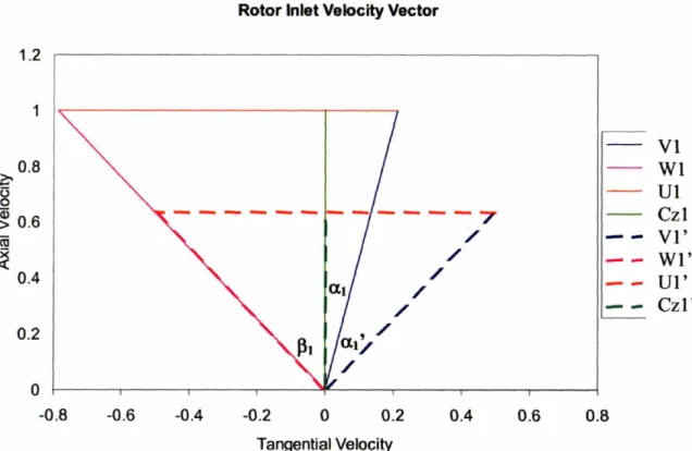
presence of the downstream diffuser ... ... 49 Figure 2-10 Rotor inlet vector diagram showing that p 1 is held constant by increasing a 1

for the quasi-2D case ... 50

Figure 2-11 Rotor inlet flow angle as a function of flow coefficient showing that the design value of 1 is maintained in the 2D model . ... 50

Figure 2-12 Impeller exit velocity diagram for the 3D and 2D cases ... 51 Figure 2-13 DeHaller number for cases the baseline (3D) inlet flow angle and the

modified (2D) inlet flow angle showing that the design DeHaller number is

maintained in the 2D model which has a flow coefficient of 0.6 ... 51 Figure 2-14 Pf along splitter chord for 2D grid study cases showing that the coarse and

medium grid with 160 timesteps-per-pass results in similar decay of the unsteady disturbance ... 52 Figure 2-15 Pf along splitter chord for 3D grid study cases shows that nearly identical

unsteadiness is observed for both the medium and fine grids ... 52

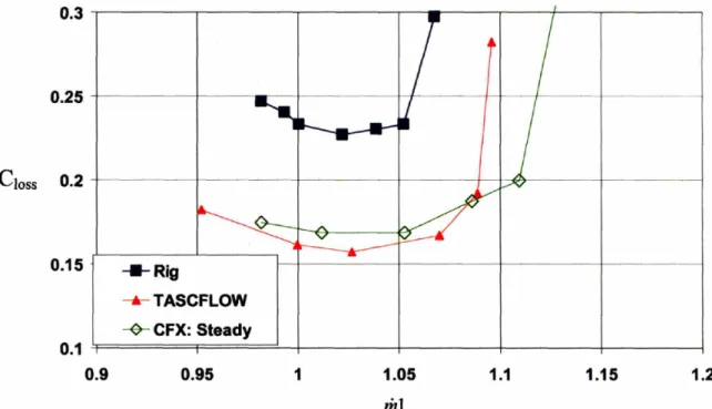
Figure 2-16 CFX computed diffuser loss compared with experimental data and

Figure 2-17 CFX computed diffuser loss compared with experimental data and

TASCFLOW computations ... ... 53 Figure 2-18 CFX computed stage pressure ratio compared with experimental data and

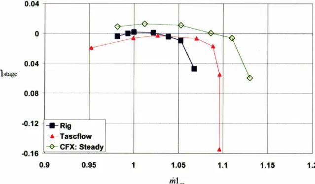
TASCFLOW computations ... 54 Figure 2-19 CFX computed stage efficiency compared with experimental data and

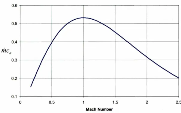
TASCFLOW computations ... 54 Figure 3-1 Corrected flow per unit area plotted against Mach number showing a peak

value of approximately 0.54 at a Mach number of 1 ... 70 Figure 3-2 Sample inlet total pressure disturbance showing differences between unsteady

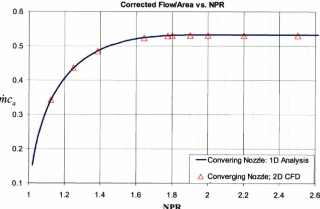
and time-averaged nozzle pressure ratio (NPR) ... 70 Figure 3-3 Corrected flow-per-unit area plotted against NPR (nozzle pressure ratio).

Case C indicates the flow based on the time-averaged NPR, while D indicated the

time-averaged flow for a quasi-steady disturbance ... 71

Figure 3-4 Sketch of the simple nozzle used for the quasi-steady analysis ... 71 Figure 3-5 Computational grid used for the unsteady CFD computations ... 72 Figure 3-6 CFX computed corrected flow against NPR, compared with 1 1D analysis.. 72 Figure 3-7 Error in steady-estimated mass flow as predicted by the quasi-steady analysis,

showing large difference are incurred at low pressure ratios ... 73 Figure 3-8 Second derivative of Corrected Flow with respect to nozzle pressure ratio ... 73 Figure 3-9 Mach Number Distribution: Pr= .1 showing approximately incompressible

flow ... 74 Figure 3-10 Mach number Distribution: Pr=1.6 showing high Mach number subsonic

flow ... 74 Figure 3-11 Mach number distribution: Pr=2.2 showing the choked conditions at the

nozzle exit ... 74 Figure 3-12 Inlet total pressure boundary conditions for the NPR=l.l cases ... 75

Figure 3-13 Inlet mass-flow-per-unit-area for the NPR=1 cases, showing a phase shift for

the higher frequency cases ... 75 Figure 3-14 CFX computed velocity magnitude compared with a 1D analysis, which

shows good agreement at low (=.1) and high (=10) ... 76 Figure 3-15 CFX computed velocity phase compared with a 1D analysis, which shows

that CFX agrees well at low frequency... 76 Figure 3-16 CFX computed difference in mass flow. The low-frequency CFD

calculations compare well with quasi-steady analysis. ... 77 Figure 3-17: Product of density and velocity perturbation showing increased magnitude

for higher-frequency cases ... 77

Figure 3-18 'Velocity and density perturbation for P =. 1 show that velocity and density

fluctuations are out of phase ... ... 78 Figure 3-19 'Velocity and density perturbation for P =10 show that velocity and density

fluctuations are in- phase, which leads to a higher time-averaged mass flow ... 78 Figure 4-1 Compressor Map computed based on the quasi-2D approximation to the

centrifugal com pressor stage... 89 Figure 4-2 Normalized static pressure distribution (Pn) for 6 instants during /2diffuser

p assin g p erio d ... 9 0

Figure 4-3 Splitter Blade Static Pressure at time instant t=2/12 T, indicating sharp

Figure 4-4 Contours of Pf for 4 cases to elucidate regions of significant unsteadiness ... 92 Figure 4-5 Contours of Pf for 4 cases showing a close-up at the impeller trailing edge to

elucidate the high levels of unsteadiness on the pressure surface trailing edge A and

B ... 93

Figure 4-6 Unsteady splitter chordwise loading distribution for case A indicating

significant blade loading variation at the leading edge region ... 94 Figure 4-7 Unsteady splitter chordwise loading distribution for case B indicating reduced

loading relative to case A, but significant loading variation at the leading edge region ... 94 Figure 4-8 Unsteady splitter chordwise loading distribution for case C showing a

significant reduction in loading near leading edge relative to case A ... 95 Figure 4-9 Unsteady splitter chordwise loading distribution for case D showing a

significant reduction in loading near the leading edge ... 95 Figure 4-10 Strength of loading fluctuation vs. distance along splitter chord, showing

differences in disturbance strength between cases A-D ... 96

Figure 4-1 1 Decay of static pressure disturbance in Vaneless Space showing the effect of increased gap on the strength of the disturbance imposed at the impeller trailing

edge ... 96

Figure 4-12 Time-Averaged normalized static pressure near diffuser leading edge shown to elucidate the decay of the static pressure disturbance in the vaneless space ... 97 Figure 4-13 Time-averaged normalized static pressure rise showing increased pressure

rise for cases A and B ... ... 98 Figure 4-14 Time-Averaged and mass averaged relative Mach number in the impeller

passage, showing lower exit Mach numbers for cases A and B ... 98

Figure 4-15 DeHaller Number in Quasi-2D Calculations ... 99 Figure 5-1 Computed impeller pressure ratio for quasi-2D cases, with closed symbols

indicating time-averaged results ... ... 108 Figure 5-2 Computed impeller efficiency for quasi-2D cases ... 108 Figure 5-3 Contour of Pf for coupled quasi-2D model of centrifugal compressor to

compare with those for the isolated impeller subjected to an imposed downstream

static pressure field ... 109

Figure 5-4 Contours of Pf for cases 8 and 9, showing strong unsteadiness for case 8, which has decreased corrected mass flow relative to case A ... 110 Figure 5-5 Chordwise loading distribution for case 5, showing strong fluctuations of

unsteady load in the leading edge region ... 110 Figure 5-6 Chordwise loading distribution for case 6, showing moderate fluctuations of

unsteady load in the leading edge region ... 111 Figure 5-7 Chordwise loading distribution for case 7, showing small fluctuations of

unsteady load in the leading edge region ... 111 Figure 5-8 Chordwise loading distribution for case 8, showing increased fluctuations of

unsteady load in the leading edge region, relative to case 5 ... 112 Figure 5-9 Chordwise loading distribution for case 5, showing moderate fluctuations of

unsteady load in the leading edge region ... 112 Figure 5-10 Strength of splitter blade loading fluctuations for cases 5-9 ... 113

Figure 5-12 L* plotted vs. DeHaller Number, showing the trend that cases with low DeHaller number (increased diffusion) exhibit increased upstream unsteadiness. 114 Figure 6-1 CFX computed stage pressure ratio, showing reasonable agreement between

experiment and time-averaged calculations ... 124 Figure 6-2 CFX computed stage efficiency, showing reasonable agreement between

experiment and time-averaged calculations ... 124 Figure 6-3 Static pressure distribution for 6 instants during Y2 diffuser passing period. 125 Figure 6-4 Flow streamlines (based on time-averaged velocity) in the diffuser entrance

region ... 126 Figure 6-5 Contours of Pf for Cases 10 and Case 11, showing moderate levels of

unsteadiness in case 10, and decreased levels of unsteadiness in case 11 ... 127

Figure 6-6 Chordwise loading distribution for case 10, showing strong loading

fluctuations at trailing edge. Moderate levels of unsteady load fluctuations can also

be observed in the leading edge region... 127

Figure 6-7 Chordwise loading distribution for case 11, showing strong loading

fluctuations at trailing edge, and negligible load fluctuations near the leading edge

... ... ... ... ... ... 12 8

Figure 6-8 Strength of unsteady loading fluctuations for cases 10 and 11, showing

stronger levels of unsteady loading in the leading edge region for case 10 ... 128 Figure 6-9 Comparison of mode shapes and load fluctuation ... 129 Figure 6-10 Impeller pressure ratio for cases A, 5, and 10, showing that the impeller

pressure ratio is similar for all three cases ... 129 Figure 6-11 Comparison of splitter unsteady loading between cases A, 9, and 10, showing

that case A has three distinct peaks while case 9 (2D isolated impeller) and case 10

(3D) have four ... ... 130

Figure 6-12 Comparison of time-averaged diffuser static pressure distribution, showing the difference between case A (2D stage model) and case 10 (3D stage model).. 130 Figure 6-13 Time-averaged and area-averaged relative Mach number along impeller

flowpath showing lower Mach numbers for Case A ... 131 Figure 6-14 Contours of Mach number and P', showing the effect of mean flow Mach

number on the spatial distribution of the static pressure disturbance. The higher Mach number in case 10 decreases the speed of the upstream traveling disturbance, thus increasing the number of peaks per splitter chord ... 132 Figure 6-15 Comparison of splitter loading fluctuation between Case A and Case 10.. 133

List of Tables

Table 2-1 Summary of Unsteady Calculations ... ... 37

Table 2-2 3D diffuser grid refinement study ... ... 40

Table 2-3 Results of 2D unsteady grid refinement study ... 41

Table 2-4 Results of 3D unsteady grid refinement study ... 42

Table 3-1 Error in mass-flow-per-unit-area between... 66

1. Introduction and Motivation

1.1 Motivation

Centrifugal compressors are widely used in industry, ranging from gas pumps, aircraft propulsion, and stationary power generation. Compressors are exposed to a variety of unsteady forces that can increase stress levels in the part, and lead to premature

structural failure. One significant source is the unsteady loading due to the presence of upstream and downstream bladerows. These time-varying loads can induce vibratory stresses in the blades that are significantly higher than the steady-state stresses. Material failure due to vibratory stresses is usually referred to as high-cycle fatigue, or HCF.

Current methods deal with the centrifugal compressor HCF problem by minimizing exposure to stimuli that excite the resonant frequencies of the compressor components. The condition where a modal frequency and a stimulus frequency coincide is referred to as a resonant crossing. Due to the large number of structural modes and potential stimuli, some resonant crossings are always present in an engine's operating range. The decision on which crossings remain in the operating range relies on past experience and

engineering judgment. Often, this leads to unexpected difficulties during initial testing of a new or fielded engine. Engine companies can spend valuable time and money fixing an HCF problem during the engine development phase. Knowledge of the aerodynamic forcing function prior to engine test would allow a design engineer to eliminate the exposure to the most severe operating conditions prior to manufacturing the initial hardware.

Thus there is a need for a research effort to understand and predict unsteady loading on the compressor components, namely blades and vanes, and the conditions under which aeromechanical difficulties such as HCF can occur. Improved understanding of the basic design variables that control the level of unsteady loading can aid in identifying crossings of concern. By defining an adequate model for predicting the time-dependent flow field, a designer would have the essential forcing function required for forced response

identification of high stress crossings so that they can be removed from the operating range. This would lead to more robust designs and significantly reduce the risk of

encountering HCF problems during the engine development phase.

1.1 Technical background

1.2.1 The centrifugal compressor

The major advantage of the centrifugal compressor over axial designs is that high pressure ratios (greater than 8:1) can be obtained in a single stage. The use of a

centrifugal compressor can greatly reduce the weight, cost, and parts count when a high pressure rise is required. Centrifugal compressors are generally used in low mass flow gas turbine applications where they can obtain high efficiency and do not require an excessively large frontal area [1].

Total pressure rise is obtained in the centrifugal compressor via two specific

mechanisms. First, aerodynamic diffusion in the relative frame results in a net increase in kinetic energy in the absolute frame. Second, there is a centrifugal force on the air that is a consequence of the increase in radius from inlet to outlet [2]. The centrifugal effect is the main differentiation between axial and centrifugal compressors. Centrifugal work transfer does not require relative frame diffusion, so the magnitude of the pressure rise is not limited by airfoil separation as in the axial compressor.

A centrifugal compressor consists of an impeller followed by a diffuser. Airflow enters the rotating impeller in the axial direction at station 1 and exits the impeller in the radial direction at station 2, as shown in Figure 1-1. Torque is transferred to the fluid via the rotating blades on the compressor disk. Often times, main (long) and splitter (short) blades are used. This allows for large flow area at the inlet, while maintaining adequate solidity for high slip factors at the exit.

Airflow leaves the impeller with high kinetic energy and high absolute Mach number. The diffuser is a stationary component consisting of radial passages that de-swirl and diffuse the high Mach number flow prior to entering the combustor. Often, a de-swirling bend section is used downstream of the main diffuser to turn the flow towards axial

before entering the combustor. Combustor stability requirements often require a substantial level of diffusion in the diffuser stage [2]. Aerodynamic losses in both the impeller and diffuser limit the overall pressure rise capability and adiabatic efficiency of the machine.

1.2.2 Compressor durability

Compressor durability refers to the ability of the compressor to withstand its

operating loads over the required mission life of the part. Durability is a critical design constraint, as it effects the safety, operational cost, and readiness of the flight vehicle system. Two common modes of material failure in a compressor are low-cycle fatigue and high-cycle fatigue.

High cycle fatigue is a phenomenon where mechanical vibration induces significant unsteady stress levels in a part. One source of vibration is forced response, where an unsteady forcing function excites a structural mode, leading to high unsteady stress

levels. Metallic materials typically have a known endurance limit, a combination of mean and alternating stress levels that the material can withstand indefinitely without

experiencing material failure. Fatigue margin can be defined as the relative difference between the peak operating stresses in a part and the known endurance limit (Figure 1-2).

In the limit where no vibratory stresses are present, the fatigue limit represents the ultimate strength of the material.

The blade mean stress is set by design variables such as material density, rotational speed, and gas temperature. Finite-element methods have been shown to provide

reasonably adequate assessments of the mean stress. The alternating, or vibratory stress is more challenging to quantify. Vibratory stress levels are set by design variables such as the material thickness, strength of the unsteady blade loading and damping forces.

Forced response analysis can be used to analytically assess the magnitude of the vibratory stresses, but an adequate representation of the forcing function is needed to obtain valid results. Partly because of this reason, current industry practice for centrifugal

1.3 Previous work

Availability of resources in high-speed computing makes three dimensional time-accurate simulations feasible for generating aerodynamic data for rotating

turbomachinery. Time accurate simulations which account for the relative motion of the rotor are essential to developing an understanding of the flow phenomena which set the levels of unsteady loading in a centrifugal stage. Consideration of previous work aids in understanding the state-of-the-art and provides a starting point for this research.

Computational fluid dynamic (CFD) simulations of centrifugal compressors have been successfully used to calculate stage performance by several researchers. Srivastava and Macrorie performed a steady-state mixing plane calculation for a centrifugal stage with a GE MOD-2 type diffuser using the Tascflow code [4]. Calculated stage

performance, in terms of pressure rise and efficiency, was within 1% of the experimental results from rig tests. Roberts and Steed also performed mixing plane calculations using CFX [5]. This stage had a "fish-tail" style pipe diffuser close-coupled to a tandem blade impeller. Results showed that CFD calculations for stage performance were also within 1% of the experimental results. Both calculations capture the trends of stage performance with operating conditions. Results from these steady state analyses provide confidence in the capability of CFD to make reasonable predictions of centrifugal compressor

performance.

In recent years, there has been an increasing focus in using CFD to calculate time-accurate flowfields in centrifugal compressors. Shum [6] quantified the effect of impeller-diffuser interaction on centrifugal stage performance. Mainly concerned with stage performance, Shum [6] identified the impeller-diffuser gap as a controlling parameter for unsteady interaction in the stage. Strong fluctuations observed in the last

10-15% of the vane passage for a baseline design with a 9% radius ratio demonstrate the upstream influence of the diffuser static pressure disturbance. Murray [7] verified Shum's findings, and put forth a hypothesis that gap-to-pitch ratio is the controlling parameter which sets the impact of unsteadiness on compressor performance. An

unsteady simulation was undertaken by Sheng [8] on a different centrifugal compressor. He showed that a Reynolds-averaged code U2NCLE provided a reasonably adequate assessment of the performance trends near the design speed.

Unsteady blade loading and its implication on HCF has been recently researched by Caitlin Smythe [9]. Smythe [9] compared the unsteady flowfield for two similar

compressor designs, one of which has known aeromechanics difficulty. Results showed that this compressor had stronger unsteady fluctuations along the blade surfaces than the baseline compressor. The use of unsteady CFD analysis for aeromechanics design was discussed by Kielb [10]. He showed that recent calculations for resonant response, including unsteady CFD, compare well with experimental measurements.

Ziegler et al performed experimental investigations of impeller-diffuser interactions in a centrifugal compressor [11]. Comparisons between two diffuser configurations showed significantly higher levels of velocity fluctuations at the impeller exit when the radius was decreased from 14% to 4%.

1.4 Selection of a research compressor

For the purpose of studying the unsteady flow field, a research centrifugal compressor is chosen. A compressor recently developed at the General Electric Company showed evidence of aeromechanics difficulty during the product development stage. Indications of HCF were found at the splitter blade leading edge. Further investigation into the problem revealed two resonant crossings in the operating range of the machine.

A Campbell diagram is commonly used to depict resonant crossings. Modal

frequencies amd stimulus frequencies are plotted on the vertical axis against rotor speed on the horizontal axis. The Campbell diagram for this particular machine shows the two modal frequencies crossing the diffuser passing frequency in the operating range (Figure

1-3). Follow on engine testing revealed high levels of vibratory response for the 6th_modal

crossing, but significantly lower levels for the 5th mode. Thus this provides a clear

indication of an upstream manifestation (indication at splitter LE) of a downstream stimulus (diffuser passing frequency).

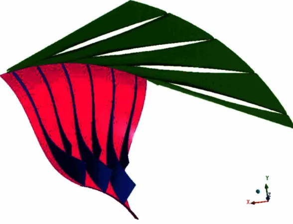
The centrifugal stage of interest consists of a backswept impeller with alternating full and partial-passage splitter blades. The stator consists of a GE Mod-2 diffuser coupled to a radial bend and a deswirl cascade (Figure 1-4). The Mod-2 diffuser is a 3-dimensional diffuser that is formed by discrete passages machined into a solid metal ring. The diffuser shape consists of several distinct sections, shown in Figure 1-5.

Investigation of the flowfield of this compressor serves to identify the conditions under which impeller-diffuser interaction action can drive high levels of vibration. Although the physical speed of the crossings occur at different values, the centrifugal compressor operating point is essentially identical for the two modes. Due to the

temperature rise which occurs in the upstream axial compressor and the fact that the two compressors run at the same physical speed, the centrifugal compressor operating line remains fixed over the range of rotor corrected speeds (Figure 1-6).

Although a design fix has been developed for this machine, the basic behavior of this machine provides a valuable source of information. Analysis of the flowfield of this machine provides insight to the link between unsteady blade loading and high vibratory stress in the airfoils.

1.5 Technical objectives

Based on the observations in the research compressor, three objectives are put forward for this research project

1) Identify the physical mechanism responsible for the observed aeromechanics phenomena and quantify the level of unsteady loads acting on the splitter blade

2) Identify the design parameters that control the level of unsteady loading in a centrifugal compressor stage

3) Define an adequate model for predicting unsteady loading in a centrifugal

1.6 Research contributions

The specific contributions of this research are: (1) First of a kind unsteady numerical experiments have been implemented to elucidate an upstream manifestation of a

downstream stimulus for a centrifugal compressor stage with a Mod-2 diffuser. (2) The controlling parameters identified are impeller-diffuser gap, stage loading (characterized by DeHaller number), and relative Mach number; the impeller-diffuser gap sets the

strength of the unsteady loading, while stage loading sets the extent of the upstream manifestation of unsteady loading. (3) The results of a quasi-2D isolated impeller model in which an unsteady static pressure boundary condition is used to approximate the presence of a downstream diffuser have been shown to capture the key features of the unsteady blade loading. (4) The effect of time-averaging the unsteady inlet conditions has been eliminated as a source of over-predictions in the choked flow capacity of a fluid device.

An implied utility of the contributions are: (i) Identification of the controlling parameters as noted in (2) can provide direction in the future when there is a need to reduce the level of unsteady loading so as to avoid occurrence of aeromechanics

difficulty; and (ii) the quasi-2D approximation could be used during the design phase to approximate the unsteady loading in a timeframe that is compatible with the design environment.

1.7 Thesis outline

This thesis is presented in the following manner:

Chapter 2:

Chapter two describes the overall approach used to analyze the unsteady flow fields in the centrifugal compressor. CFX is assessed and showed to be an adequate computational tool for performing the unsteady calculations.

Chapter 3:

Chapter 3 is focused on assessing the impact of unsteady flow on the choked flow capacity of a simple nozzle. The goal is to confirm whether unsteady effects play a role in the over-prediction of choked flow when steady-state approximations are used. Results from quasi-steady analysis and unsteady CFD show that there is no inherent unsteady, inviscid effect that leads to over-predictions of choked flow when steady methods are used.

Chapter 4:

Chapter 4 presents the results of quasi-2D unsteady analysis of the centrifugal stage. Four specific diffuser geometries are considered (baseline, increased throat, increased gap, increased gap and throat). The results are synthesized in order to identify the key parameters that control the level of flow unsteadiness in a centrifugal stage.

Chapter 5:

Chapter 5 presents the results from a quasi 2-D unsteady analysis of a centrifugal impeller. An unsteady pressure boundary condition is used to simulate the presence of the downstream diffuser. The goal of this analysis is to assess the hypothesis that operating conditions effect the attenuation of an unsteady disturbance. Specifically, increased mass flow and the resulting decreased diffusion leads to enhanced upstream attenuation of the unsteady pressure disturbance in the impeller passage.

Chapter 6:

Chapter 6 presents the results of the 3-D unsteady calculation of the research compressor at the design point. The peak levels and upstream extent of the unsteady load on the splitter blade is quantified. Unsteady blade loading computed from the quasi 2-D model is shown to be in accord with the unsteady blade loading computed from the full

Chapter 7:

Chapter 7 provides a summary of the research and provides suggestions for future work.

1

Figure 1-1 Sketch of centrifugal compressor, showing stations 1,2 and 3 which delineate the impeller inlet, impeller exit, and diffuser exit respectively

lade stress

0.8

Generic Goodman Diagram

1.2 ,----,---,----,----,----,---n .. Blade Stress - Fatigue Limit 0.2 -I---l--"=---..---1---+---I---~~--_____1 Alternating Stress 0.6 0.4 -1---1----+---+---""""'=-1----1.2 0.8 0.6 0.4 0.2 0+----+----..---.---1---.1f---=l o Mean Stress

Campbell Diagram Splitter Vane Modes

Inlet Guide Vanes

1.2 0.8 0.4 0.2 '" - M6: Baseline

/

/

/

/

---

--

---P-

~-

Figure 1-3 Campbell diagram for the research compressor showing the diffuser frequency crossing the 5tb

and 6tb

modal frequencies of the splitter

Figure 1-5 MOD-2 diffuser cross-sections which indicate the complex 3D nature of the diffuser design

Centrifugal Operating Parameters Sea-level Static Standard Day

~eded Speed <>

I

Figure 1-6 Centrifugal compressor corrected speed and flow vs. rotor speed showing small changes in operating parameters for a range of physical speeds

2. Technical Approach

2.1 Introduction

This chapter describes the methodology used in performing the numerical

experiments required to address the research questions posed in chapter 1. Section 2.2 provides a description of the computational tool utilized for these experiments, and the method used to reduce the data into relevant metrics. Section 2.3 describes the specific models used for the computational experiments. Section 2.4 presents the results of code assessment studies for the models described in section 2.3. The models are first checked for numerical adequacy, and then compared with measured rig data. Results of these studies show that the selected tool is adequate for answering the research questions.

2.2 Computational Tool

2.2.1 Description of CFX code

Computational fluid dynamics (CFD) is selected as a tool to analyze the unsteady flowfield of the research compressor. The results are used to extract physical

understanding and identify the specific flow process of interest. CFD can be used during the design phase to provide valuable insight in to the unsteady flow behavior prior to testing a new design

The commercial code CFX 5.7.11 has been used for all calculations described in this thesis. CFX is a finite-volume based flow solver that solves the set of equations for 3D unsteady compressible flow over a discretised fluid domain. The control-volume form of the 5 conservation equations (mass, momentum (3), and energy) is applied at

finite volumes formulated at each node in the discretised domain. CFX uses a fully implicit coupled iterative solver that updates flow variables until all conservation

equations are satisfied within a specified tolerance. Second order accuracy is obtained by a "numerical advection correction" which uses a gradient-based correction for

approximating primitive variables at integration points. A second-order backwards Euler scheme is used to approximate transient terms. The use of CFX for calculating turbo machinery rotor-stator flow has been reported in a paper by Galpin, et al [12].

Turbulence is modeled using the shear-stress transport (SST) model. SST is a Reynolds-averaged turbulence modeling approach that accounts for the turbulent stresses by representing only the mean quantities in a flow field [13]. SST combines the k-s and the k-o turbulence models via a blending function which forces k-o in the boundary layer and k-s in the freestream. This method has been shown to produce acceptable and consistent results for a wide range of mesh sizes[ 14].

2.2.2 Computational Grid

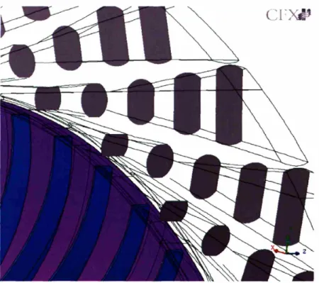
The numerical procedure described in section 2.2.1 requires an adequate grid to represent the fluid device of interest. The grid used to model the research compressor is shown in Figure 2-1. This figure shows the grid on a section through the mid-span of the impeller and the diffuser. Structured hexahedral elements are used on the impeller, while unstructured tetrahedral elements are used on the diffuser. Generating an adequate structured grid for the diffuser proves difficult due to the complex 3D shape, so the unstructured grid has been chosen. Unstructured mesh has been shown to provide adequate results by several researchers [5,6,8]. Figure 2-2 shows a cross-section of the mesh at the diffuser throat. Note the incorporation of inflation layers near the walls in order to adequately model the shear layer in the wall region.

2.2.3 Boundary Conditions

Boundary conditions must be specified at all boundaries of the grid where specific conditions are known. Inlet boundary conditions consist of specifying the total pressure, total temperature and flow angle. These conditions are based on measurements from the

experimental rig. Physical mass flow is specified at the domain exit, except near choke conditions where static pressure is specified.

Boundary conditions must also be specified on the surfaces in the domain that represent rigid walls. In general, walls are specified as smooth, no-slip walls that are

fixed in the appropriate reference frame. The one exception is wall boundaries for the quasi-2D model. In this case, the model uses a thin cut through the passage, and free-slip walls are used on lower and upper boundaries spanning between the blade surfaces.

Blades in a compressor are usually evenly spaced, thus the flow in the compressor exhibits blade-to-blade periodicity. In other words, the flow field can be represented by multiple repeated sections. One can take advantage of this fact and significantly reduce the memory requirements for a model. A periodic boundary is applied at surfaces-of-revolution that bound a single impeller passage. These boundary conditions forces flow

variables to be equal at corresponding nodes.

One additional boundary condition that requires some attention is the interface between the impeller and the diffuser. In order to calculate a steady solution, an

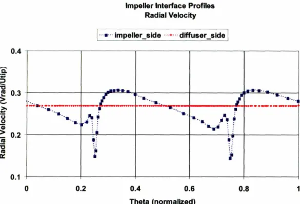
approximation is made. The CFX stage (also known as mixing plane) model is chosen to approximate the flow at the diffuser inlet. Mixing plane uses an averaging procedure to mix-out the impeller exit profile in order to develop average boundary conditions at the diffuser inlet.. Density, radial velocity, tangential velocity, and static temperature are averaged across the interface in a manner that conserves mass flow, radial momentum, tangential momentum, and energy across the interface. Figure 2-3 shows circumferential distribution of radial velocity at the impeller-diffuser interface. Note that the impeller profile is mixed-out to a uniform velocity imposed on the downstream diffuser. The physical implication of mixing plane is that the static pressure influence of the diffuser is not passed into the impeller, and thus unsteady effects are not accounted for. Figure 2-4 shows the circumferential distribution of static pressure at the interface. Note that the static pressure profile at the impeller is not reflective of the downstream static pressure disturbance at the inlet to the diffuser. The mixing plane formulation is used to obtain an initial condition for unsteady calculations and to estimate the stage performance, but cannot be used to obtain the unsteady blade loading.

In order to assess the unsteady blade loading, multiple time-accurate simulations are performed. Rather than averaging flow variables across the interface, the sliding plane formulation is used at the impeller-diffuser interface. Sliding plane directly maps flow quantities across the interface using an interface grid. Relative motion between the impeller and diffuser is accounted for by updating the position of the impeller relative to the diffuser for each timestep.

Pitch differences are accounted for by scaling flow quantities across the interface. In other words, the interface grid is "stretched" or "compressed" in the circumferential direction when the impeller blade and diffuser passage counts differ. The physical implication is that the wavelength of the diffuser disturbance does not replicate the true wavelength. Therefore, all unsteady models use 3 impeller passages and 4 diffuser passages. This ratio of impeller blades and diffuser passages is assumed to closely

approximate the full geometry. The geometry used for the unsteady calculation is depicted in Figure 2-5.

2.2.4 Data-Reduction Method

All post-processing is performed with CFX POST. Eight governing equations are used to solve for 8 primitive flow variables for each interior node. All derived variables,

such as Mach number, total pressure, total temperature, and entropy can be calculated from the primitive variables.

p from Conservation of mass

Ux from Conservation of momentum (x-direction) Uy from Conservation of momentum (y-direction) Uz from Conservation of momentum (z-direction) H from Conservation of energy

Ts from Constitutive equation (dH=Cp*dT)

k from Turbulent kinetic energy transport o from Turbulent frequency transport

Compressor performance is calculated for all steady state and transient cases. For all cases where time-accurate flow simulations are used, time-averaging followed by mass-averaging is used to calculate the operating point and overall performance of the machine. Time averaging of a flow variable at a given node is given by

i=m

I i

=i0r (eq 2.1)

where 4 is the averaged value, 4 is the instantaneous value corresponding to time-instant i, m is the number of timesteps included in the time averaging, and X is the

characteristic period over which the variable is time-averaged. This period represents the time required for the splitter blade to proceed from a diffuser vane leading edge to the next, referred to as the diffuser passing period.

Mass averaging of is obtained by using

N

(PiVVi dAi)oi

# ma = iNO (eq 2.2)

(Vi dAi )

i=O

where s ma is the averaged quantity, N is the total number of nodes on the surface of

interest, is the surface normal vector, dAiis the area of a surface bounding the finite

volume at a given node i, and Xi is the time-averaged flow quantity at the given node i. 6 major metrics are used to quantify machine performance at a given operating condition. Impeller pressure ratio, i,, is given by

wimp = 2na/pt m (eq 2.3)

while impeller efficiency is given by

-1

rimp -= T

-

where temperature ratio, timp, is given by

Timp Tt2 / T t (eq 2.5)

Temperature ratio represents the amount of work needed to obtain the pressure ratio, rimp . Pressure ratio and efficiency define the overall performance and are two

major design parameters for a compressor.

Diffuser performance is defined by the pressure recovery and pressure loss coefficient. The goal of the diffuser is to convert the high dynamic pressure at the impeller exit into high static pressure. The recovery coefficient, Cp,

PSma _ Pma

P P2ma _ psma (eq. 2.6)

represents the fraction of the available dynamic pressure that is recovered. Pressure loss

coefficient, Closs,

pt2ma j Pt ma

represents the reduction in total pressure due to irreversible processes that occur in the diffuser.

The overall performance of the stage accounts for the impeller performance and additional losses that occur in the diffuser. Stage pressure ratio, restage,

Jstage Pt3 /Ptl (eq 2.8)

represents the net pressure ratio created in the stage, including losses in the diffuser.

Stage efficiency, Tistage,

r-1

stage r-l

Ofstage - t g (eq 2.9)

imp

represents the ratio of ideal temperature rise for the given pressure rise to the actual temperature ratio required.

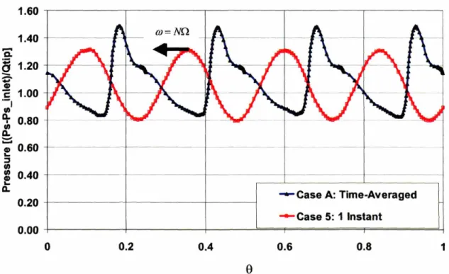
Several additional variables are calculated from the CFD results to quantify the unsteady behavior in the stage. A metric for quantifying the level of unsteadiness, Pf, is defined as

Px -P.,r

.5p1U 2

where P,r and P,,r represent the maximum and minimum static pressure which occur during one characteristic period, respectively. Pf represents the strength of unsteadiness by comparing the peak-to-peak pressure fluctuations. The time-accurate load across the splitter blade is of utmost interest because this sets the level of peak strain, and thus has strong implications for aeromechanics response. The expression for splitter loading is given by

AP = PPS - Pss (eq 2.11)

'5p U2

where PpS and P,, represent the static pressure on the pressure and suction side of the splitter, respectively. This equation uses the time-accurate static pressure difference across the blade at a given streamwise location. A metric for quantifying the level of load fluctuations on the blade, ALs, is given by

ALs = APs -APs (eq 2.12)

where AP,.r and AP,,r represent the maximum and minimum load that occurs during 1 characteristic period, respectively.

2.3 Technical Framework

2.3.1 Structured numerical experiment

Four sets of numerical experiments (denoted as Parts I, II, III, and IV) are

designed and implemented for addressing the three research questions posed in chapter 1. The results are interrogated and assessed in a manner that serves to answer the research questions.

Part I constitutes a set of steady-state mixing plane calculations of the research compressor at the design speed. The calculation is performed for a range of corrected mass flowrates from stall to choke. Part I is required for two specific reasons. First, the results of the calculations are compared with experimental rig data to provide a

quantitative assessment of the code. Second, a converged steady state solution is required to provide initial conditions for the unsteady calculation.

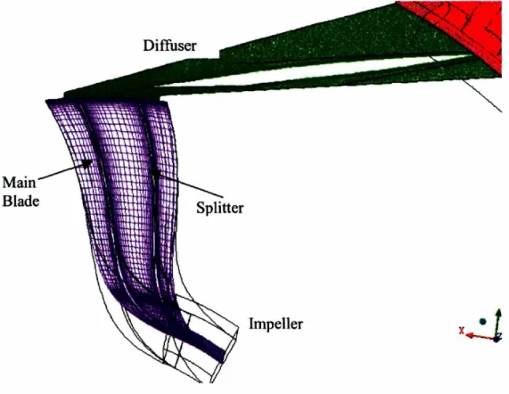
With code assessments complete, CFX can then be used to perform unsteady calculations. Part II consists of four quasi-2D unsteady stage calculations. A thin cut

through the impeller and diffuser meanline is used to approximate the compressor geometry. Figure 2-6 shows the model. It can be seen that the geometry is

representative of the research compressor. Impeller blade and diffuser vane angles are maintained. Scaling of hub and casing profiles maintain the impeller stream-wise area distribution. Impeller-diffuser gap and diffuser pitch is also maintained. This model is

referred to as case A.

The quasi-2D model is chosen for unsteady analysis for several reasons. First, it includes the unsteadiness associated with the interaction of the diffuser inlet static pressure disturbance with the upstream rotating impeller. A simpler model allows for clearer interpretation of the results. Second, the computational effort is significantly reduced relative to a full 3D unsteady model. Comparison of 2D and 3D calculations are performed to determine if a 2D model is adequate for estimating the unsteady loads. This is done to confirm if the 2D approximation is acceptable for estimating the loading.

Because the 2D model includes the unsteadiness associated with the interaction of the diffuser inlet static pressure disturbance with the upstream rotating impeller, it is used to identify parameters that control the level of unsteady loading in a centrifugal

compressor stage. Two parameters are chosen for study, one being the impeller-diffuser gap and the other the diffuser throat area. Thus, three additional perturbations on the baseline diffiser geometry are modeled in part II. Case B uses the baseline throat, but an impeller-diffilser gap that is twice that of the baseline (denoted as 2X gap). Case C uses the baseline gap, but a diffuser throat area that is 20% greater than that of the baseline

(denoted as 1.2X throat). Case D has a 2X gap with a 60% increase in throat. The goal

of case D is to investigate the combined effect of increasing these two parameters. Figure 2-7 shows the solid models for the four 2-D diffuser configurations analyzed. It shows the change in gap between case A and B and the change in throat between case A and C.

Results from part II show clear differences in unsteady loading with increased throat, but the effect of throat cannot be isolated from the effect of corrected mass flow. Therefore, part III of the study is used to isolate the effect of corrected mass flow on unsteady loading. Figure 2-8 shows the computational grid used in part III. It shows that the impeller model is identical to part II, but the diffuser geometry is removed from the

model. Presence of the diffuser is simulated via an unsteady static pressure boundary condition at the impeller exit,

P (,t) = P + psin(2r

_-

₎

_{(eq 2.13)}

Ni

where Ps is the mean static pressure (varied in order to set the mass flow), ap is the magnitude of the static pressure disturbance, N is the number of diffuser vanes, M is the number of impeller blades, 0 is the circumferential location, and is the diffuser passing frequency, defined as

o= N (eq 2.14)

where QC is the rotational speed of the impeller in radians/sec. The value for ap is selected in order to match the strength of the static pressure disturbance at the meanline as calculated by the 3D mixing plane calculation. Figure 2-9 shows the circumferential variation of static pressure. It shows how equation 2.14 results in a harmonic wave that represents the static pressure disturbance at the impeller-diffuser interface plane.

While calculations from part II and III provide useful results on unsteady loading in a centrifugal compressor, they are obtained using a simple model of the actual

compressor. Thus there is a need to implement full 3D unsteady calculations at the design point and this constitutes Part IV. Interrogation of this final calculation serves several purposes. First, the unsteady time-averaged performance is compared with experimental rig data as an additional step in code assessment. Second, the unsteady loading on the impeller blade is quantified. Third, the unsteady behavior is compared to the 2D model results to determine if the 2D model is adequate for calculating unsteady loads.

Comparison of the unsteady results from parts II, III, and IV provide valuable unsteady data that is used to answer the research questions. Table 2-1 provides a summary of all of the calculations discussed in this section. For reference, several variables that characterize the operating condition are included. The mass flow shown is

the computed corrected mass flow per unit area normalized by the design point value, herein referred to as "mass flow". al is the absolute frame inlet flow angle (relative to the design point), while

P1

Table 2-1 Summary of Unsteady Calculations

2.3.2 Implication of mass flow and incidence angle changes on impeller loading

Development of the quasi-2D model results in one parameter that cannot be set to the same value as the 3D model, that being the impeller inlet-to-diffuser throat area ratio. The ratio of impeller-inlet to diffuser throat is decreased by 40% in the 2D model. This is a consequence of the 3D geometry of the diffuser. Because the diffuser width increases with radius, a thin cut through the meanline results in a lower diffuser inlet area for a

Calculation Part Diffuser Dim Cc i pi

A II A 2D .68 36.5 -0.5 B II B 2D .65 36.5 1.7 C II C 2D .78 36.5 -10.8 D II D 2D .89 36.5 -24.0 5 III N/A 2D .69 36.5 -1.7 6 III N/A 2D .77 36.5 -9.5 7 III N/A 2D .89 36.5 -24.0 8 III N/A 2D .57 36.5 8.8 9 III N/A 2D 1.00 0 0 10 IV A (3-D) 3D 1.05 0 -1.0 11 IV A (3-D) 3D 1.10 0 -3.0

given impeller inlet area. Thus the mass-flow-per-unit area at the impeller inlet is reduced to perform the 2-D calculation.

In order to maintain similar flow conditions in the impeller, the rotor inlet angle, p1, must be maintained. Velocity components for the rotor inlet velocity vector, is shown in Figure 2-10. Velocity components denoted with solid lines represent the design point, while the dashed line represent the vector diagram for the quasi-2D model. It shows that an equivalent 1 is achieved by adjusting the absolute frame flow angle to maintain P1 at the lower mass flow. Rotor inlet angle can be calculated using the inverse tangent function

Af = tan-'1( ) (eq 2.15)

c.,

and an expression for Wo, in terms of known variables Czl, U₁, and al

WO1= U1- U 1 (eq 2.16)

Combining equations 2.15 and 2.16 results in an expression for 1 in terms of know quantities

,I = tan-' ( tana,) (eq 2.17)

where 0, referred to as the flow coefficient, is defined as

0= C~, (eq 2.18)

U1

Figure 2-11 shows the variable 11 (normalized by the reference value) plotted against flow coefficient for two different values of al. This figure illustrates how

absolute frame incidence angle is increased in order to maintain the design value of 1 at a lower inlet mass flow.

The decrease in corrected mass flow also affects the rotor exit velocity vector, as shown in Figure 2-12. Assuming that the slip factor does not change, the relative frame exit angle, 2, is identical for both cases because the rotor metal angle remains fixed. One implication of this change is that relative frame diffusion(W2/Wi), also known as the DeHaller number, is similar for both cases. This is illustrated by considering the exit relative frame velocity,

W2= Cz2cot(p2) (eq 2.19)

which is expressed in terms of the exit flow velocity Cz2and the relative frame flow angle, and the inlet frame velocity

W = CZ j1 +2

tan(a)

_2.20)

to arrive at an expression for the DeHaller number in terms of known variables

Dehaller = C2 cot(f₂) (eq 2.21)

C,

1 +

2

tan(a

) tanan2

(a)

The DeHaller number is shown in Figure 2-13. It shows that at the 2D flow coefficient of 0.6, the DeHaller number is identical to the DeHaller number of the 3D model at a flow coefficient of 1.0, which is the design point.

The reduced mass flow capacity of the 2D coupled model is due to the difficulty in maintaining the same diffuser throat to impeller inlet area ratio when using a 2D stream tube approximation. This difficulty is overcome in 2 ways. First, the absolute frame incidence angle is adjusted to obtain impeller incidence angles and stage loading similar to the 3D case. Second, in part III of the calculations, the diffuser is removed from the calculation and corrected mass flow per-unit-area can be set to the same value as the 3D design (calculation 9).

2.4 Results of Code Assessment Studies

2.4.1 Grid Refinement studies

2.4.1.1 3D steady results

Grid refinement studies for the impeller have been previously studied on this machine by Srivastva and Macrorie [4]. Three grid refinement levels have been performed, and stage performance in terms of pressure rise and efficiency has been compared. Calculated performance has been shown to be similar for the medium and the

fine grids. Therefore, the medium grids for the impeller and deswirler grids are used. Grid refinement studies are required for the diffuser grid. Table 2-2 below summarizes the diffuser performance for three levels of grid refinement. The results show that changes in grid size do not cause significant changes in diffuser performance, so the again medium grid is selected for all studies.

Elements Cp A co A

Coarse 340K .834 .172

Medium 540K .837 +.003 .169 -.003

Fine 970K .845 +.008 .161 -.008

Table 2-2 3D diffuser grid refinement study, where K referrers to thousands.

2.1.1.1 2D unsteady results

Similar grid refinement studies were carried out for the quasi-2D model. The unsteady calculation is performed on the baseline grid at the design point. The numerical timestep is set to 16 steps per blade pass. The calculation is performed with finer timestep

calculation is then performed with the medium grid. Peak values of Pf are used to measure the initial strength of the disturbance, and upstream (20-40% chord) values are used to measure the level of decay that occurs in the impeller passage. Time-averaged efficiency is assessed to ensure that calculated performance variation is within acceptable limits.

Table 2-3 summarizes the results for all unsteady grid refinement studies.

Comparison of the second and third calculations shows small differences between the 160 and 320 timesteps-per-blade pass. Midspan Pf values are with 0.10 units, and time-averaged efficiency is within 0.24 points. Based on this calculation, the numerical

timestep of 160 timesteps-per-bladepass is deemed adequate for this unsteady calculation. This is consistent with timestep studies performed by Sheng [8]. The calculation is then performed with a grid that is twice as fine as the baseline grid, referred to as the medium

grid. The results show midspan Pf values within 0.18 units and efficiency within 0.40 points of the baseline case with 160 timesteps-per-bladepass. Figure 2-14 shows the variable Pf along the splitter chord for the four calculations performed in this grid study. It shows that the decay of the static pressure disturbance is similar for the baseline grid (denoted as triangles) and the medium grid (denoted as an asterisk). Based on these results, the baseline impeller grid with 160 timesteps-per-period is chosen for all analyses.

Elements Timestep Impeller Diffuser Mid Peak Efficiency (impeller)

Pf A Pf A imp A

38.6K T/16 Base Base .14 1.49 5.73

38.6K T/160 Base Base .60 .46 1.62 .13 5.32 -.41

38.6K T/320 Base Base .70 .10 1.72 .10 5.56 .24

lOOK T/160 Med Base .78 .18 1.43 -.19 5.72 .40 Table 2-3 Results of 2D unsteady grid refinement study

Although the 3D impeller grid is shown to be adequate for steady flow, this does not imply that it would be adequate for unsteady flows. Therefore, additional unsteady grid refinement studies are performed on the impeller. Table 2-4 contains the results for the 3D study. It shows that results are similar for both the medium and fine cases. Midspan Pf values are within 0.01 units and peak Pf values are identical. Figure 2-15 shows Pf along the splitter chord (both pressure and suction surfaces), and illustrates that both the medium and fine grid result in similar decay of the static pressure disturbance. Based on this study, the medium grid is chosen for the 3D unsteady calculations.

Elements Timestep Impeller Diffuser Mid Peak Efficiency (impeller)

Pf A Pf A A

1 660K T/160 Base Base 0.16 1.00 -1.09

2 1.3M T/160 Med Base 0.30 .14 0.92 0.8 -1.28 -0.19

3 2.1M T/160 Fine Base 0.29 -.01 0.92 0.0 -1.24 0.04 Table 2-4 Results of 3D unsteady grid refinement study, where M stands for millions

2.4.2 Steady state performance trends

Having demonstrated that the computational model of the stage is adequate, the next step is to assess the calculated steady-state stage performance against experimental data obtained in a test rig. The research compressor has been tested in a rig facility at GE Aircraft Engines in Lynn, MA. A calibrated venturi has been used to measure mass

flowrate, and total pressure/temperature rakes have been used to measure pressure and temperatures at the impeller inlet, impeller exit, and the deswirler exit.

Figure 2-16 and Figure 2-17 show diffuser loss coefficient and recovery coefficient, respectively. Both figures show that the results of CFX are similar to previous calculations performed in TASCFLOW. TASCFLOW is a computational tool previously used at GE Aircraft Engines for calculation centrifugal compressor

performance. TASCFLOW has been shown to provide an adequate assessment for centrifugal compressor flow, and therefore provides a baseline that can be used to assess CFX [4,12]. Both the magnitude and trend with inlet corrected flow are reproduced. CFX results for diffuser performance are in accord with previously calculated results. Both figures suggest that the CFD codes over predict the performance. The results do show that both CFD codes reproduce the performance trend as mass flow is varied.

Figure 2-18 and Figure 2-19 show stage pressure ratio and efficiency,

respectively. Note that these variables have been normalized by the measured design point values. Both figures indicate that the performance trends are similar to both the TASCFLOW and measured rig data. The overall level is somewhat over-predicted by CFX, but within a reasonable range. Stage pressure ratio is approximately 3% higher at the design point, and efficiency is approximately one point higher at the design point.

Steady-state analysis of the stage indicates that of both the diffuser performance and the overall performance of the stage are approximately in line with measured values. Both the trends with corrected flow and the overall levels are in reasonable agreement. Based on this assessment, CFX is deemed adequate for capturing the relevant flow processes in the research compressor.

2.5 Summary

The technical framework for addressing the research questions posed in chapter 1 is presented in the chapter. The framework consists of designing and implementing steady and unsteady simulations of flow in an impeller-diffuser stage. A quasi-2D

representation of the impeller-diffuser is used in order to achieve a significant reduction in required computational resources. Four diffuser designs with varying impeller-diffuser gap and diffuser throats are considered. In addition, an isolated impeller with an imposed downstream static pressure field is designed in order to isolate the effect of corrected mass flow. Results of several code assessment studies indicate that the selected tool is adequate for assessing the flowfield for the selected research compressor. In the following chapters, the results are to be interrogated in order to address the research

Main Blade

Figure 2-1 Computational grid for the research compressor which shows the structured grid used to model the impeller

CF

Figure 2-2 Cross-section of grid at diffuser throat which has unstructured tetrahedral elements in the passage, but utilizes inflation layers on the diffuser walls.