An RMS for Non-predictably Evolving Applications

HAL Id: inria-00599150

https://hal.inria.fr/inria-00599150v3

Submitted on 9 Jun 2011

HAL is a multi-disciplinary open access

archive for the deposit and dissemination of

sci-entific research documents, whether they are

pub-lished or not. The documents may come from

teaching and research institutions in France or

abroad, or from public or private research centers.

L’archive ouverte pluridisciplinaire HAL, est

destinée au dépôt et à la diffusion de documents

scientifiques de niveau recherche, publiés ou non,

émanant des établissements d’enseignement et de

recherche français ou étrangers, des laboratoires

publics ou privés.

Cristian Klein, Christian Pérez

To cite this version:

Cristian Klein, Christian Pérez. An RMS for Non-predictably Evolving Applications. [Research

Report] RR-7644, INRIA. 2011. �inria-00599150v3�

a p p o r t

d e r e c h e r c h e

An RMS for Non-predictably Evolving Applications

Cristian KLEIN and Christian PÉREZ

N° 7644 — version 3

Centre de recherche INRIA Grenoble – Rhône-Alpes 655, avenue de l’Europe, 38334 Montbonnot Saint Ismier

Téléphone : +33 4 76 61 52 00 — Télécopie +33 4 76 61 52 52

Cristian KLEIN and Christian PÉREZ

Domaine : R´eseaux, syst`emes et services, calcul distribu´e ´

Equipe-Projet GRAAL / Avalon

Rapport de recherche n° 7644 — version 3 — initial version 8 June 2011 — revised version 9 June 2011 — 25 pages

Abstract: Non-predictably evolving applications are applications that change their resource require-ments during execution. These applications exist, for example, as a result of using adaptive numeric methods, such as adaptive mesh refinement and adaptive particle methods. Increasing interest is being shown to have such applications acquire resources on the fly. However, current HPC Resource Man-agement Systems (RMSs) only allow a static allocation of resources, which cannot be changed after it started. Therefore, non-predictably evolving applications cannot make efficient use of HPC resources, being forced to make an allocation based on their maximum expected requirements.

This paper presents CooRMv2, an RMS which supports efficient scheduling of non-predictably evolving applications. An application can make “pre-allocations” to specify its peak resource usage. The application can then dynamically allocate resources as long as the pre-allocation is not outgrown. Resources which are pre-allocated but not used, can be filled by other applications. Results show that the approach is feasible and leads to a more efficient resource usage.

pour les applications évolutives

R´esum´e : Les applications évolutives non-prédictibles sont des applications dont les besoins en ressources changent en cours d’exécution. Leurs comportements proviennent, par exemple, des méth-odes numériques adaptatives, comme le raffinement de maillage adaptatif et les méthméth-odes de particules adaptatives. Il y a un intérêt croissant à ce que ce type d’application acquiert des ressources à la volée. Cependant, les gestionnaires de ressources haute performance (HPC) ne supportent qu’une allocation sta-tique des ressources, qui ne peut donc pas changer après le démarrage de l’application. Par conséquence, les applications évolutives non-prédictibles ne peuvent pas utiliser les ressources HPC de manière efficace, car elles sont forcées de faire une demande de ressources en fonction de leurs pics de besoins.

Cet article présente CooRMv2, un gestionnaire de ressources qui permet l’ordonnancement efficace d’applications évolutives non-prédictibles. Une application peut faire des « pré-allocations » pour ex-primer ses pics de besoins en ressources. Ensuite, l’application peut dynamiquement allouer de manière sûre des ressources tant que la pré-allocation n’est pas dépassée. Les ressources pré-allouées, mais inutil-isées, sont à la disposition des autres applications. Les résultats montrent que l’approche est réalisable et que l’utilisation des ressources est améliorée.

Mots-cl´es : gestion des ressources; supercalculateurs; grappes de calcul; applications évolutives; malléabilité.

Contents

1 Introduction 4

2 A Model for Non-Predictably Evolving Applications 4

2.1 Working Set Evolution Model . . . 4

2.2 A Speed-up Model . . . 5

2.3 Analysis of the Model . . . 6

3 CooRMv2 7 3.1 Principles . . . 7 3.1.1 Requests . . . 7 3.1.2 Request Constraints . . . 7 3.1.3 High-Level Operations . . . 8 3.1.4 Views . . . 8 3.2 RMS Implementation . . . 9 3.3 Example Interaction . . . 10 4 Application Support 10 5 Evaluation 11 5.1 Application and Resource Model . . . 11

5.1.1 AMR Application . . . 11

5.1.2 Parameter-Sweep Application (PSA) . . . 12

5.1.3 Resource Model . . . 12

5.2 Scheduling with Spontaneous Updates . . . 12

5.3 Scheduling with Announced Updates . . . 13

5.4 Efficient Resource Filling . . . 14

6 Related Work 14 6.1 Malleable . . . 15 6.2 Evolving . . . 15 7 Conclusion 15 8 Acknowledgments 16 A RMS Implementation 18 A.1 Requests . . . 18

A.2 Request Constraints . . . 18

A.3 Views . . . 19

A.4 Helper Functions . . . 19

A.4.1 toView() . . . 20

A.4.2 fit() . . . 21

A.4.3 eqSchedule() . . . 21

A.5 Main Scheduling Algorithm . . . 24

1

Introduction

High-Performance Computing (HPC) resources, such as clusters and supercomputers, are managed by a Resource Management System (RMS) which is responsible for multiplexing resources among multiple users. Generally, computing nodes are space-shared, which means that a user gets an exclusive access. Requesting a resource allocation is mostly done using rigid jobs: the user requests a number of nodes for a limited duration, then the RMS decides when the allocation is served.

Increased interest has been devoted to giving more flexibility to the RMS, as it has been shown to improve resource utilization [1]. If the RMS can reshape a request, but only before the allocation starts, the job is called moldable. Otherwise, if the RMS can change the allocation while it is served, the job is called malleable. Taking advantage of moldable jobs often comes for free, as commonly used programming models (e.g., MPI) are already suitable for creating moldable applications. However, writing malleable applications is somewhat more challenging as the application has to be able to reconfigure itself during execution. How to write malleable applications [2, 3] and how to add RMS support for them [4, 5, 6] has been extensively studied.

Improving utilization can be done further by supporting evolving applications. These are applications which change their resource requirements during execution as imposed by their internal state. Unlike malleability, the change of the resource allocation is not imposed by the RMS, but by the nature of the computations. Being able to provide applications with more nodes and memory on the fly is considered necessary for achieving exascale computing [7].

We define three types of evolving applications: (i) fully-predictable, whose evolution is known at start (e.g., static workflows), (ii) marginally-predictable (e.g., non-DAG workflows containing branches), whose evolution can only be predicted within a limited horizon of prediction, and (iii) non-predictable, whose evolution cannot be known in advance. Non-predictably evolving applica-tions (NEA) are more-and-more widespread, due to the increased usage of adaptive numeric methods, such as Adaptive Mesh Refinement (AMR) [8] and Adaptive Particle Methods (APM) [9].

Unfortunately, support for evolving applications is insufficient in current RMSs. In batch schedulers, evolving applications are forced from the beginning to allocate enough resources to fulfill their peak requirements. In Clouds, which support dynamic provisioning, large-scale resource requests may be refused with an “out-of-capacity” error, thus, allocating resources on the fly may lead to the application reaching an out of memory condition.

This paper proposes CooRMv2 an RMS that enables efficient scheduling of evolving applications, especially non-predicable ones. It allows applications to inform the RMS about their maximum expected resource usage (using pre-allocations). Resources which are pre-allocated but unused can be filled by malleable applications.

The main contribution of the paper is three-fold: (i) to devise a model for NEAs based on AMR applications; (ii) to propose CooRMv2 an extension to our previous RMS, for efficiently supporting such applications; (iii) to show that the approach is feasible and that it can lead to considerable gains.

The remaining of this paper is organized as follows. Section 2 motivates the work and refines the problem statement by presenting a model of an AMR application. Section 3 introduces CooRMv2, a novel RMS which efficiently supports various types of applications as shown in Section 4. Section 5 evaluates the approach and highlights the gains that can be made. Section 6 discusses related work. Finally, Section 7 concludes the paper and opens up perspectives.

2

A Model for Non-Predictably Evolving Applications

This section presents a model of a non-predictably evolving application based on observations of AMR applications. First, the evolution of the working set size and the speed-up of the application are modeled. Second, the model is analyzed and the problem statement is refined.

2.1

Working Set Evolution Model

Our goal is to devise a model for simulating how the data size evolves during an AMR computation. In order to have a model which is parametrizable, we first devise a “normalized” evolution profile, which is independent of the maximum size of the data and the structure of the computations. The model has

0 100 200 300 400 500 600 700 800 900 1000 0 100 200 300 400 500 600 700 800 900 1000

Normalized data size

Step number

Figure 1: Examples of obtained AMR working set evolutions.

to be simple enough to be easy to analyze and use, but at the same time it should resemble observed behaviors. To this end, we consider that the application is composed of 1000 steps. During step i the size of the data si is considered constant (si∈ [0, 1000]).

Unfortunately, we have been able to find only a few papers on the evolution of the refined mesh. Most of the papers focus either on providing scalable implementations [10] or showing that applying AMR to a certain problem does not reduce its precision as compared to a uniform mesh [8]. From the few papers we found [11, 12], we extracted the main features of the evolution: (i) it is mostly increasing; (ii) it features regions of sudden increase and regions of constancy; (iii) it features some noise.

Using the above constraints, we derive the following model, that we call the acceleration-deceleration model. First, let the evolution of the size of the mesh be characterized by a velocity vi, so that

si = si₋₁+ vi. The application is assumed to be composed of multiple phases. Each phase consists of

a number of steps uniform randomly distributed in [1, 200]. Each step i of an even phases increases vi

(vi= vi−1+ 0.01), while each step i of an odd phases decreases vi (vi= vi−1× 0.95). Next, a Gaussian

noise of µ = 0 and σ = 2 is added. The above values have been chosen so that the profiles resemble the ones found in the cited articles. At the end, the profile is normalized, so that the maximum of the series

si is 1000.

To obtain the actual, non-normalized data size profile Si at step i, given the maximum data size

Smax, one can use the following formula: Si = si× Smax. Figure 1 shows some examples of data size evolutions returned by the model, which are compatible with those presented in [11, 12].

2.2

A Speed-up Model

The next issue is to find a function t(n, S) that returns the duration of a step, as a function of the number of allocated nodes n and the size of the data S. Both n and S are assumed constant during a step.

Instead of having a precise model (such as in [13]) which would be applicable to only one AMR application, we aimed at finding a simple formula, which could be fit against existing data. To this end, we chose to use the data presented in [14] as it shows both strong and weak scalability of an AMR application for data sizes which stay constant during one experiment. After trying several functions and verifying how well they could be fit, we found a good one to be:

t(n, S) = A×S

n+ B× n + C × S + D

The terms of this formula can be intuitively explained. Term A expresses the part of the computation which is perfectly parallelisable. Term B is the overhead of the parallelization, such as the extra effort to keep track of all the nodes in the system or the extra cost of collective communication. Term C is the time payed by each nodes per unit of data, the limiting factor for a good weak scalability. Finally, D is a constant term.

Figure 2 presents the result of logarithmically fitting this formula against actual data. The model fits within an error of less than 15% for any data point. The values of the parameters, used in the rest of the paper, are: A = 7.26× 10−3_{s× node × MiB}−1_{, B = 1.23× 10}−4_{s× node}−1_{, C = 1.13× 10}−6_{s× MiB}−1_,

1 10 100 1 4 16 64 256 1k 4k 16k Duration of a step (s) Number of nodes 3136 GiB 784 GiB 196 GiB 48 GiB 12 GiB

Figure 2: Fitting the AMR speed-up model against the actual data for different mesh sizes.

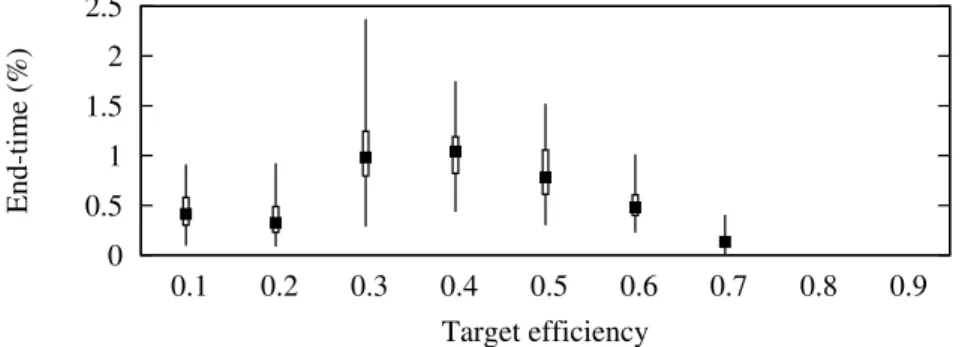
0 0.5 1 1.5 2 2.5 0.1 0.2 0.3 0.4 0.5 0.6 0.7 0.8 0.9 End-time (%) Target efficiency

Figure 3: End-time increase when an equivalent static allocation is used instead of a dynamic allocation.

2.3

Analysis of the Model

Let us analyze the model and refine the problem statement. Users want to adapt their resource allocation to a target criterion. For example, depending on the computational budget of a scientific project, an application has to run at a given target efficiency. This allows scientists to receive the results in a timely fashion, but at the same time control the amount of used resources.

To run the above modeled application at a target efficiency etthroughout its whole execution, given

the evolution of the data size Si, one can compute the number of nodes ni that have to be allocated

during each step i of the computation. Let us denote the consumed resource area (node-count×duration)

in this case A(et). In practice, while executing the application, one does not need any a priori knowledge

of the size of the data, as ni only depends on the current Si.

However, most HPC resource managers do not support dynamic resource allocations, which forces a user to request a static number of nodes. Let us define the equivalent static allocation a number of nodes neq which, if assigned to the application during each step, leads to the consumed resource area

A(et). Computing neq requires to know all Si a priori. Using simulations, we found that neq exists for

et < 0.8. Of course, with a static allocation, some steps of the application run more efficiently, while

others run less efficiently than et. However, interestingly, the end-time of the application increases with

at most 2.5% (Figure 3). We deduce that, if users had an a priori knowledge of the evolution of the data size, they could allocate resources using a rigid job and their needs would be fairly well satisfied.

Unfortunately, the evolution of an AMR application is generally not known a priori, which makes choosing a static allocation difficult. Let us assume that a scientist wants to run her application efficiently. E.g., she wants her application not to run out of memory, but at the same time, she does not want to use 10% more resources than A(75%). Figure 4 shows the range of nodes the scientist should request, depending on the maximum data size Smax. We observe that taking such a decision without knowing the

evolution of the application in advance is difficult, in particular, if the behavior is highly unpredictable. Ideally, a distinction should be made between the resources that an evolving application expects to use in the worst case and the resources that it actually uses. The unused resources should be filled by malleable applications, that can free these resources if the evolving application requests them. However, since applications might belong to different users, this cannot be done without RMS support. The next section proposes such an RMS.

1/8 1/4 1/2 1 2 4 8 0 1000 2000 3000 4000 5000

Data size (relative)

Number of hosts

Figure 4: Static allocation choices for a target efficiency of 75%.

3

CooRMv2

This section introduces CooRMv2, an RMS which allows to efficiently schedule malleable and evolving applications, whether fully-, marginally- or non-predictable. First, it explains the concepts that are used in the system (Section 3.1). Second, an RMS implementation is proposed (Section 3.2). The section concludes by showing an example of interaction between the RMS, a malleable application and an evolving application (Section 3.3).

3.1

Principles

At the core of the RMS-Application interaction are four concepts: requests, request constraints, high-level operations and views. Let us detail each one of them.

3.1.1 Requests

A request is a description, sent by applications to the RMS, of the resources an application wants to have allocated. As in usual parallel batch schedulers, a request consists of the number of nodes (node-count), the duration of the allocation and the cluster on which the allocation should take place1_{. It is} the RMS that computes a start-time for each request. When the start-time of a request is the current time, node IDs are allocated to the request and the application is notified.

CooRMv2 supports the following three request types. Non-preemptible requests (also called run-to-completion, default in most RMSs [16]) ask for an allocation that once started cannot be interrupted by the RMS. Preemptible requests ask for an allocation that can be interrupted by the RMS, whenever it decides to, similar to OAR’s best-effort jobs [17].

In order to allow a non-predictably evolving application to inform the RMS about it’s maximum expected resource usage, CooRMv2 supports a third request type which we shall call pre-allocation. No node IDs are actually associated with the request, the goal of a pre-allocation being to allow the RMS to mark resources for possible future usage. In order to have node IDs allocated, an application has to submit non-preemptible requests inside the pre-allocation. Pre-allocated resources cannot be allocated non-preemptibly to another application, but they can be allocated preemptibly.

Section 4 shows that these types of requests are sufficient to schedule evolving and malleable appli-cations.

3.1.2 Request Constraints

Since CooRMv2 deals with applications whose resource allocation can be dynamic, each application is allowed to submit several requests, so as to allow it to express varying resource requirements. However, the application needs to be able to specify some constraints regarding the start-times of the requests relative to each other. To this purpose, each request r has two more attributes: relatedTo—points to an existing request (noted rp)—and relatedHow—specifies how r is constrained with respect to rp.

CooRMv2 defines three possible values for relatedHow (Figure 5): FREE, COALLOC, and NEXT. FREE means that r is not constrained and relatedTo is ignored. COALLOC specifies that r has to start at the

Figure 5: Visual description of request constraints (Section 3.1.2).

(a) Initial state (b) Spontaneous (c) Announced

Figure 6: Performing an update.

same time as rp. NEXT is a special constraint that specifies that r has to start immediately after rp,

with r and rp sharing common resources. If r requests more nodes that rp, then the RMS will allow

the application to keep the resources allocated as part of rp and will send additional node IDs when r is

started. If r requests fewer nodes than rp, then the application has to release node IDs at the end of rp.

3.1.3 High-Level Operations

Let us now examine how applications can use the request types and constraints to fulfill their need for dynamic resource allocation.

Having defined the above request types and request constraints, the targeted applications only need two low-level operations: request() adds a new request into the system, while done() immediately terminates a request (i.e., its duration is set to the current time minus the request’s start-time) and, for requests constrained with NEXT, specifies which node IDs have been released. Using these two operations, an application can perform high-level operations. We shall present two of which are the most relevant: spontaneous update and announced update.

A spontaneous update is the operation through which an application immediately requests the allocation of additional resources. It can be performed by calling request() with a different node-count, then calling done() on the current request. Given the initial request state in Fig. 6(a), Fig. 6(b) shows the outcome of a spontaneous update.

An announced update is the operation through which an application announces that it will require additional resources at a future moment of time (i.e., after an announcement interval has passed), thus allowing the system (and possible other applications) some time to prepare for the changes of resource allocation. It can be performed by first calling request() with a node-count equal to currently allocated number of nodes and a duration equal to the announcement interval, then calling request() with a new node-count and, finally, calling done() on the current request (see Figure 6(c)).

Note that, in order to guarantee that at update is successful (i.e., the RMS can allocate additionally requested resources), updating non-preemptible requests can only be guaranteed if they can be served from a pre-allocation.

3.1.4 Views

For the targeted applications, simply sending requests to the RMS is not enough. Applications need to be able to adapt their requests to the availability of the resources. For example, instead of requesting a large number of nodes which are available only at a future time, a moldable application might want to request fewer nodes to reduce its waiting time, thus reducing its end-time.

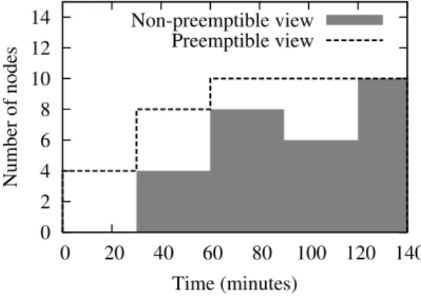
0 2 4 6 8 10 12 14 0 20 40 60 80 100 120 140 Number of nodes Time (minutes) Non-preemptible view Preemptible view

Figure 7: Example of views for one cluster.

To this end, the RMS provides each application a view containing the current and future availability of resources. Views should be regarded as the current information that the RMS has, but should not be taken as a guarantee. Applications can scan their view and estimate when a request would be served by the RMS. This helps moldable applications as they do not need to emulate the scheduling algorithm of the RMS. When the state of the resources changes, the RMS will push new views to the applications, so that they can update their requests, if necessary.

On a more technical note, a view stores for each cluster a step function, that stores the cluster availability profile: the x-axis is the absolute time and the y-axis is the number of available nodes as illustrated in Figure 7.

In CooRMv2, two types of views are sent to each application i: non-preemptive (V_¬P(i)) and preemptive view (V_P(i)). The former allows applications to estimate when pre-allocations and non-preemptive requests will be served, while the latter allows it to estimate when non-preemptive requests will be served.

The preemptive view is also used to signal an application, that it has to release some preemptively allocated resources, either immediately or at a future time. In CooRMv2, each application is supposed to cooperate and immediately release node IDs when it is asked to, using the above presented update operation. Otherwise, if a protocol violation is detected, the RMS kills the application’s processes and terminates the session with it.

3.2

RMS Implementation

This section presents an RMS implementation that we have realized. A CooRMv2 RMS has three tasks: (i) for each application i compute a non-preemptible (V_¬P(i)) and a preemptible view (V_P(i)), (ii) compute the start-time of each request and (iii) start requests and allocate node IDs.

For briefness, only a high-level description of the implementation is given. The RMS runs a scheduling algorithm whenever it receives a request or done message. In order to coalesce messages coming from multiple applications at the same time and reduce system load, the algorithm is run at most once every re-scheduling interval, which is an administrator-chosen parameter. A value for this parameter is given in Section 5.

The scheduling algorithm goes as follows. Applications are sorted in a list based on the time the applications connected to the RMS. First, pre-allocation requests are scheduled using Conservative Back-Filling (CBF) [18]. Next, inside these pre-allocations, non-preemptible requests are scheduled. Non-preemptible requests which cannot be served from allocations are implicitly wrapped in pre-allocations of the same size. The remaining resources are used to schedule preemptible requests.

Regarding preemptive views and the start-time of preemptive requests, they are computed so as to achieve equi-partitioning. However, should an application not use its partition, other applications are allowed to fill it in.

The proposed scheduling algorithm has a linear complexity with respect to the number of requests in the system. We have developed a Python implementation (with more compute-intensive parts in C++)

Figure 8: Example of an interaction between the RMS, a Non-predictably Evolving Application and a Malleable Application.

which is able to handle approximately 500 requests/second on a single core of an Intel® _{Core™2 Duo} CPU @ 2.53 GHz.

The above implementation is just one possible implementation and can easily be adapted to other needs. For example, the amount of resources that an application can pre-allocate can be limited, by clipping its non-preemptible view.

3.3

Example Interaction

Let us describe the RMS-Application protocol using an example. Assume there is one NEA and one malleable application in the system (see Figure 8). First, the NEA connects to the RMS (step 1). In response, the RMS sends the corresponding views to the application (step 2). The NEA sends a pre-allocation (step 3) and a first non-preemptible request (step 4), to which the RMS will immediate allocate resources (step 5). Similar communication happens between the RMS and the malleable application, except that a preemptible request is sent (step 6–9). As the computation of the NEA progresses, it requires more resources, therefore, it performs a spontaneous update (step 10–11). As a result, the RMS updates the view of the malleable application (step 12), which immediately frees some nodes (step 13–14). Then, the RMS allocates these nodes to the NEA (step 15).

4

Application Support

This section evaluates how the CooRMv2 architecture supports the types of application presented in Section 1.

A rigid application sends a single non-preemptible request of the user-submitted node-count and duration. Since the application does not adapt, it ignores its views.

A moldable application waits for the RMS to send a non-preemptive view, then runs a resource selection algorithm, which choses a non-preemptible request. Should the state of the system change before the application starts, the RMS shall keep it informed by sending new views. This allows the application to re-run its selection algorithm and update its request, similarly to CooRM [19].

A malleable application first sends a non-preemptible request rminwith its minimum requirements.

Next, for the extra resources (i.e., the malleable part), the application scans its preemptive view VP and

sends a preemptible request rextra, which is COALLOCated with rmin. rextra can either request a

only the resources it can actually take advantage of. For example, if the malleable application requires a power-of-two node-count, but 36 nodes are available in its preemptive view, it can request 32 nodes, leaving the other 4 to be filled by another application. During execution, the application monitors VP

and updates rextra if necessary.

A fully-predictably evolving application sends several non-preemptible requests linked using the NEXT constraint. During its execution, if from one request to another the node-count decreases, it has to call done with the node IDs it chooses to free. Otherwise, if the node-count increases, the RMS sends it the new node IDs.

A non-predictably evolving application (NEA) first sends a pre-allocation request (whose node-count is discussed below), then sends an initial non-preemptible request. During execution, the applica-tion updates the non-preemptible request as the resource requirements change. Since such updates can only be guaranteed as long as they happen inside a pre-allocation, such an application may adopt two strategies: sure execution or probable execution.

The application can opt for a sure execution, i.e., uninterrupted run-to-completion, if it knows the maximum node-count (nmax) it may require. To adopt this strategy, the size of the pre-allocation must

be equal to nmax. In the worst case, nmax is the whole machine.

Otherwise, if the application only wants probable execution, e.g., because pre-allocating the max-imum amount of required resources is impractical, then the application sends a “good-enough” pre-allocation and optimistically assumes never to outgrow it. If at some point the pre-pre-allocation is insuffi-cient, the RMS cannot guarantee that updates will succeed. Therefore, the application has to be able to checkpoint. It can later resume its computations by submitting a new, larger pre-allocation. Note that, in this case, the application might further be delayed as the RMS might have placed it at the end of the waiting queue.

If multiple NEAs enter the system two situations may occur. Either their pre-allocations are small enough to fit inside the system simultaneously, in this case the NEAs are launched at the same time, or their pre-allocations are too large to fit simultaneously, in which case the one that arrived later will be queued after the other. In both cases, the RMS is able to guarantee that whenever one of the NEAs requests an update inside its pre-allocation, it can actually be served. Resources that are pre-allocated to a NEA, but not allocated, cannot be non-preemptively allocated to another application. However, these resources can be filled by the malleable part of other applications. This approach is evaluated in the next section.

5

Evaluation

This section evaluates CooRMv2. First, the application and resource models are presented. Next, the impact on evolving and malleable applications is analyzed.

The evaluation is based on a discrete-event simulator, which simulates both the CooRMv2 RMS and the applications. To write the simulator, we have first written a real-life prototype RMS and synthetic applications. Then, we have replaced remote calls with direct function calls and calls to sleep() with simulator events.

5.1

Application and Resource Model

As other works which propose scheduling new types of application [6], we shall only focus on the mal-leable and evolving applications, which can fully take advantage of CooRMv2’s features. Therefore, we shall not evaluate our system against a trace of rigid jobs [20] as is commonly done in the community. Nevertheless, as shown in Section 4, the proposed system does support such a usage.

For the evaluation, two applications are used: a non-predictably evolving AMR and a malleable parameter-sweep application. Let us present how the two applications behave with respect to CooRMv2. 5.1.1 AMR Application

A synthetic AMR application is considered, which behaves as a non-predictably evolving application with a sure execution (see Section 4). The application knows its speed-up model, but cannot predict how the working set will evolve (see Section 2). Knowing only the current working set size, the application tries to target an efficiency of 75% using spontaneous updates.

The user submits the application by trying to “guess” the node-count neq of the equivalent static

allocation (defined in Section 2). The application uses this value for its allocation. Inside this pre-allocation, non-preemptible allocations are sent/updated, so as to keep the application running at the target efficiency.

Since the user cannot determine neq a priori, her guesses will be different from this optimum.

There-fore, we introduce as a simulation parameter the overcommit factor, which is defined as the ratio between the node-count that the user has chosen and the best node-count assuming a posteriori knowl-edge of the application’s behavior.

5.1.2 Parameter-Sweep Application (PSA)

Inspired by [21], we consider that this malleable applications is composed of an infinite number of single-node tasks, each of duration dtask. As described in Section 4, the PSA monitors its preemptive view. If

more resources are available to it than it has currently allocated, it updates its preemptive request and spawn new processes. If the RMS requires it to release resources immediately, it kills a few tasks then updates its request. The computations done so far are lost. We measure the PSA waste which is the number of node-seconds wasted in such a case.

If the RMS is able to inform the PSA in a timely manner that resources will become unavailable, then the PSA waits for some tasks to complete, afterwards it updates its request to release the resources on which the completed tasks ran. No waste occurs in this situation.

5.1.3 Resource Model

We assume that resources consist of one single, large homogeneous cluster of n nodes. The re-scheduling interval of the RMS is set to 1 second, to obtain a very reactive system.

5.2

Scheduling with Spontaneous Updates

This experiment evaluates whether CooRMv2 solves the initial problem of efficiently scheduling NEAs. Two applications enter the system: one AMR and one PSA (P SA1with dtask= 600 s). Since we want

to highlight the advantages that supporting evolving applications in the RMS brings, we shall schedule the AMR application in two ways: dynamic, in which the application behaves as described above, and static, in which the application is forced to use all the resources it has pre-allocated.

Regarding the resources, the number of nodes n is chosen so that the pre-allocation of the AMR appli-cation can succeed. By observing the behaviour of the appliappli-cation during some preliminary simulations, we concluded that for an overcommit factor of φ, having n = 1400× φ is sufficient.

Figure 9 shows the results of the simulations. Regarding the amount of resources effectively allocated to the AMR (AMR used resources), the figure shows that as the overcommit factor grows, a static allo-cation forces the appliallo-cation to consume more resources. This happens because, as the user chooses more nodes for the application than optimal, the application runs less efficiently. Moreover, the application is unable to release the resources it uses inefficiently to another application.

In contrast, a dynamic allocation allows the AMR application to cease resources it cannot use ef-ficiently. Therefore, as the overcommit factor grows, a dynamic allocation allows the application to maintain an efficient execution. Note however, that thanks to the pre-allocation, if the resource require-ments of the application increase, the application can request new resources and the RMS guarantees their timely allocation. Since, CooRMv2 mandates that preemptible resources be freed immediately, the impact on the AMR application is negligible.

In this experiment, the RMS allocates the resources that are not used by the AMR application to the malleable PSA. However, since the AMR application does spontaneous updates and the RMS cannot inform the PSA in a timely manner that it has to release resources, the PSA has to kill some tasks, thus, computations are wasted (Figure 9 bottom). Nevertheless, we observe that the amount of resources wasted is smaller that the resources which would be used by an inefficiently running AMR application.

The PSA waste first increases as the overcommit factor increases, then stays constant after the overcommit factor is greater than 1. This happens because once the AMR application is provided with a big enough pre-allocation, it does not change the way it allocates resources inside it.

0 10M 20M 30M 40M 50M 60M 70M 0.1 1 10

AMR used resources (node

×

s)

AMR overcommit factor Static Dynamic 0 100k 200k 300k 400k 500k 600k 0.1 1 10

PSA waste (node

×

s)

AMR overcommit factor Dynamic

Figure 9: Simulation results with spontaneous updates.

To sum up, this experiment shows that, with proper RMS support, resources can be more efficiently used, if the system contains predictably evolving applications. Nevertheless, PSA waste is non-negligible, therefore, the next section evaluates whether using announced updates makes sense to reduce this waste.

5.3 Scheduling with Announced Updates

This section evaluates whether using announced updates can improve resource utilization. To this end, the behavior of the AMR application has been modified as follows. A new parameter has been added, the announce interval: instead of sending spontaneous updates, the application shall send announced updates (see Section 3.1.3). The node-count in the update is equal to the node-count required at the moment the update was initiated. This means that the AMR receives new nodes later than it would require to maintain its target efficiency. If the announce interval is zero, the AMR behaves as with spontaneous updates. Otherwise, the application behaves like a marginally-predictably evolving application.

For this set of experiments, we have set the overcommit factor to 1. The influence of this parameter has already been studied in the previous section.

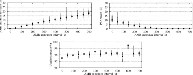
Using announced updates instead of spontaneous ones has several consequences. On the negative side, the AMR application is allocated fewer resources than required, thus, its end-time increases2 _(see Figure 10). On the positive side, this informs the system some time ahead that new resources will need to be allocated, thus, it allows other applications more time to adapt.

Figure 10 shows that the PSA waste is decreasing as the announce interval increases. This happens because, in order to free resources, the PSA can gracefully stop tasks when they complete, instead of having to kill them. Once the announce interval is greater than the task duration dtask, no PSA waste

occurs.

Let us discuss the percent of used resources, which we define as the resources allocated to appli-cations minus the PSA waste as a percentage of the total resources. Figure 10 shows that announced updates do not generally improve resource utilization. This happens because the PSA cannot make use of resources if the duration of the task is greater than the time the resources are available to it. In other words, the PSA cannot fill resources unused by the AMR if the “holes” are not big enough: these “holes” are either wasted on killed tasks or released to the system. However, the higher the announce interval, the more resources the PSA frees, so that the RMS can either allocate them to another application (see next section), or put them in an energy saving mode.

We observe that the percent of used resources has two peaks, when the announce interval is 300 s and 600 s. In these two cases, a “resonance” occurs between the AMR and the PSA. The “holes” left by the AMR have exactly the size required to fit a PSA task. On the contrary, when the announce interval is just below the duration of the task (i.e., 550 s) the percent of used resources is the lowest, as the PSA has to kill tasks just before they end.

The resource utilisations shown in the graphs are higher than typically found in today’s computing centers, however, it has been shown that these values can easily be obtained using malleable jobs [1].

2_{Instead of sending the currently required node-count in the update, the application could use linear predictions and}

send a larger announced update. However, such an approach would increase the resource usage. This approach is outside the scope of this article.

0 5 10 15 20 25 30 0 100 200 300 400 500 600 700

AMR end-time increase (%)

AMR announce interval (s)

0 5 10 15 20 25 30 0 100 200 300 400 500 600 700 PSA waste (%)

AMR announce interval (s)

96 97 98 99 100 0 100 200 300 400 500 600 700 Used resources (%)

AMR announce interval (s)

Figure 10: Simulation results with announced updates.

98 99 100

0 100 200 300 400 500 600 700

Used resources (%)

AMR announce interval (s) Strict equi-partitioning

Equi-partitioning

Figure 11: Simulation results for two PSAs.

5.4

Efficient Resource Filling

In the previous section, we have observed that while announced updates reduce PSA waste, they do not improve resource utilization. This happens because the PSA’s task duration is greater than the “holes” left by the AMR. In this section, we evaluate whether CooRMv2 is able to allocate such resources to another PSA, with a smaller task duration, in order to improve resource utilization.

To this end, we add another PSA in the system (P SA2with dtask= 60 s). By default, the RMS does

equi-partitioning between the two PSA applications, however, when one of them signals that it cannot use some resources, the other PSA can request them.

To highlight the gain, we compare this experimental setup with an RMS which implements “strict” equi-partitioning: instead of allowing one PSA to fill the resources that are not requested by the other PSA, the RMS presents both PSAs a preemptible view, which makes them request the same node-count. Figure 11 shows the percent of used resources. For readability, only medians are shown. Experiments show that CooRMv2 is able to signal P SA2 that some resources are left unused by P SA1. Resource utilization is improved, because P SA2 is able to request these resources and do useful computations on them.

To sum up, CooRMv2 is able to efficiently deal with the applications it has been designed for: evolving and malleable. On one hand, evolving applications can efficiently deal with their unpredictability by separately specifying what their maximum and what their current resource requirements are. Should evolving applications be able to predict some of their evolution, they can easily export this information into the system. On the other hand, malleable applications are provided with this information and are able to improve resource usage.

6

Related Work

To our knowledge, Feitelson [22] was the first to distinguish applications with dynamic resource usage into those that initiate the change themselves (evolving) and those that adapt to RMS’s constraints

(malleable). Unfortunately, they are often ambiguously called “dynamic” applications in literature [6, 23]. Let us review RMSs which support these types of applications.

6.1

Malleable

ReSHAPE [6] is a framework for efficiently resizing iterative applications. After each iteration, ap-plications report performance data to the RMS and the RMS attempts to divide resources, so as to optimize global speed-up. However, ReSHAPE assumes that all iterations of an application are identical and caches performance data. Therefore, applications whose iterations are irregular, such as AMR or APM applications, cannot be efficiently scheduled. Even if performance history were regularly flushed, ReSHAPE targets a specific type of applications, whereas CooRMv2 also deals with other types of malleable application.

More general support for malleability can be found in KOALA [21]. Applications declare their minimum resource requirements, then the RMS divides the “extra” resources equally (equi-partitioning). The approach is appealing and has been successfully applied to scheduling Parameter-Sweep Applications (PSA) on idle resources. However, the minimum requirements are fixed at submittal and cannot be changed during the execution. Therefore, this solution cannot be used to schedule evolving applications. The OAR batch scheduler supports low-priority, preemptible jobs called best-effort. If there are insufficient resources to serve a normal job, best-effort jobs are killed after a grace period. Best-effort jobs can be used to support malleability [5], therefore, this type of job has inspired CooRMv2’s preemptible requests. However, best-effort jobs are killed even if only part of the allocated resources need to be freed. In contrast, CooRMv2 allows an application to update its preemptible request and to free only as many resources as needed.

6.2

Evolving

In the Cloud Computing context, where consumed resources are payed for, great interest has been shown for applications that dynamically adapt their resource allocation to internal constraints [24]. However, most papers in this field only study how applications should adapt their resource requests, without studying how the RMS should guarantee that these resources can actually be allocated. Indeed, large-scale Cloud deployments can refuse an allocation request with an “out of capacity” error [25].

The Moab Workload Manager supports so-called “dynamic” jobs [23], which are both evolving and malleable: the application can grow/shrink both because its internal load changes and because the RMS asks it to. Moab regularly queries each application what its current load is, then it decides how resources are allocated. This feature has been mainly thought for interactive workloads and is not suitable for batch workloads. For example, if two non-predictably evolving applications arrive at the same time, instead of running them simultaneously, it might be better to run one after the other, so as to guarantee that peak requirements can be met. Also, Moab’s interface does not allow marginally- or fully-predictable applications to present their estimated evolution to the system.

In contrast, CooRMv2 allow an application to pre-allocate resources, so that the RMS can guarantee their availability when the application needs them. If two applications potentially require a large amount of resources, they shall be executed one after the other, to guarantee their completion. An application which can predict its evolution can export this information into the system, so as to optimize resource usage.

7 Conclusion

This paper presented CooRMv2, an RMS architecture which offers a simple interface to support various types of application, among others, malleable and fully-/marginally-/non-predictably evolving. Exper-iments showed that, if applications take advantage of the RMS’s features, resource utilization can be improved a lot, while guaranteeing that resource allocations are always satisfied.

Future work can be divided in two directions. First, it would be interesting to study how accounting should be done in CooRMv2, so as to determine users to efficiently use resources. Second, CooRMv2 was designed for managing homogeneous clusters and assumes that the choice of node IDs can be left to

the RMS. However, supercomputers feature a non-homogeneous network [26], therefore, an extension to CooRMv2 should allow network-sensitive applications to optimize their placements on such platforms.

8

Acknowledgments

This work was supported by the French ANR COOP project, n◦ANR-09-COSI-001-02.

Experiments presented in this paper were carried out using the Grid’5000 experimental testbed, being developed under the INRIA ALADDIN development action with support from CNRS, RENATER and several Universities as well as other funding bodies (https://www.grid5000.fr).

References

[1] J. Hungershofer, “On the combined scheduling of malleable and rigid jobs,” in SBAC-PAD, 2004, pp. 206–213.

[2] K. El Maghraoui, T. J. Desell et al., “Dynamic malleability in iterative MPI applications,” in

CCGRID, 2007, pp. 591–598.

[3] J. Buisson, F. André et al., “A framework for dynamic adaptation of parallel components,” in

PARCO, 2005, pp. 65–72.

[4] J. Buisson, O. Sonmez et al., “Scheduling malleable applications in multicluster systems,” Core-GRID, Tech. Rep. TR-0092, 2007.

[5] M. C. Cera, Y. Georgiou, O. Richard, N. Maillard et al., “Supporting malleability in parallel archi-tectures with dynamic CPUSETs mapping and dynamic MPI,” in ICDCN, 2010.

[6] R. Sudarsan and C. J. Ribbens, “ReSHAPE: A framework for dynamic resizing and scheduling of homogeneous applications in a parallel environment,” CoRR, vol. abs/cs/0703137, 2007.

[7] J. Dongarra et al., “The international exascale software project roadmap,” IJHPCA, vol. 25, no. 1, pp. 3–60, 2011.

[8] Adaptive Mesh Refinement: Theory and Applications. Springer, 2003.

[9] D. R. Welch, T. C. Genoni, R. E. Clark, and D. V. Rose, “Adaptive particle management in a particle-in-cell code,” Journal of Computational Physics, vol. 227, no. 1, pp. 143–155, 2007. [10] C. Burstedde et al., “Extreme-scale AMR,” in SC, 2010.

[11] D. F. Martin, P. Colella et al., “Adaptive mesh refinement for multiscale nonequilibrium physics,”

Computing in Science and Eng., vol. 7, pp. 24–31, 2005.

[12] G. L. Bryan, T. Abel, and M. L. Norman, “Achieving extreme resolution in numerical cosmology using adaptive mesh refinement: Resolving primordial star formation,” in SC, 2001.

[13] D. J. Kerbyson, J. H. Alme et al., “Predictive performance and scalability modeling of a large-scale application,” in SC, 2001.

[14] J. Luitjens and M. Berzins, “Improving the performance of Uintah: A large-scale adaptive meshing computational framework,” in IPDPS, 2010.

[15] H. Casanova, “Benefits and drawbacks of redundant batch requests,” Journal of Grid Computing, vol. 5, no. 2, 2007.

[16] D. G. Feitelson, L. Rudolph, and U. Schwiegelshohn, “Parallel job scheduling – a status report,” in

JSSPP, 2004.

[17] N. Capit, G. Da Costa et al., “A batch scheduler with high level components,” CoRR, vol. abs/cs/0506006, 2005.

[18] A. W. Mu’alem and D. G. Feitelson, “Utilization, Predictability, Workloads, and User Runtime Estimates in Scheduling the IBM SP2 with Backfilling,” TPDS, vol. 12, no. 6, pp. 529–543, 2001. [19] C. Klein and C. P´erez, “Untying RMS from Application Scheduling,” INRIA, Research Report

RR-7389, 2010.

[20] “The parallel workloads archive.” [Online]. Available: http://www.cs.huji.ac.il/labs/parallel/ workload

[21] O. O. Sonmez et al., “Scheduling strategies for cycle scavenging in multicluster grid systems,” in

CCGRID, 2009, pp. 12–19.

[22] D. G. Feitelson and L. Rudolph, “Towards convergence in job schedulers for parallel supercomput-ers,” in JSSPP, 1996.

[23] Adaptive Computing Enterprises, Inc., “Moab workload manager administrator guide, version 6.0.2.” [Online]. Available: http://www.adaptivecomputing.com/resources/docs/mwm

[24] S. Vijayakumar, Q. Zhu, and G. Agrawal, “Automated and dynamic application accuracy manage-ment and resource provisioning in a cloud environmanage-ment,” in GRID, 2010, pp. 33–40.

[25] “Lessons learned building a 4096-core cloud HPC supercomputer.” [Online]. Available: http://blog.cyclecomputing.com/2011/03/cyclecloud-4096-core-cluster.html

[26] N. R. Adiga, M. A. Blumrich et al., “Blue Gene/L torus interconnection network,” IBM J. Res.

A

RMS Implementation

This section gives details about the implementation of the RMS, which has been briefly presented in Section 3.2. First, the manipulated data structures are described in detail, next the pseudo-code of the implementation is given.

A.1 Requests

Requests (defined in Section 3.1.1) stored inside the RMS have two types of attributes: those sent by the application and those set by the RMS. The attributes which are sent by the application are:

• cid – the ID of the cluster; • n – the number of nodes;

• duration – the duration of the allocation;

• type – the type of the request: pre-allocation (P A), non-preemptible (¬P ) or preemptible (P );

• relatedHow – the type of constraint: FREE, NEXT or COALLOC; • relatedTo – the request to which the start-time is constrained.

While computing a schedule, the RMS sets the following additional request attributes: • nalloc – the number of nodes that will be effectively allocated (see details below); • scheduledAt – the time at which the allocation of this request should start; • fixed – the request is fixed, see Section A.4.1;

• earliestScheduleAt – earliest time when the request can be scheduled, see Section A.4.2. To store information about requests after they started, the RMS sets the following attributes:

• startedAt – time when the request has started; if the request has not started yet, e.g., it has just been sent by the application, this attribute is set to NaN; started(r) returns true if the request has been started.

• nodeIDs – the node IDs that have been allocated to this request.

Let us explain the purpose of the nallocattribute. Assume there are two applications in the system: a malleable application A and an evolving application B. Let us assume the following scenario. A scans its preemptive view, finds out that additional resources are available for it and updates its preemptible request. At the same time, B needs more nodes, so it spontaneously updates its non-preemptible request. The changes induced by the two applications trigger the scheduling algorithm of the RMS. Due to the race between A and B, if insufficient resources are available for both applications, then the RMS cannot allocate the requested node-count to A. Therefore, in order to correctly compute new views and request start-times, nAlloc stores the number of nodes which A can be allocated according to the current resource state. When a preemptible request is started, nAlloc is used to decide how many node IDs to allocate. nalloc might be smaller than n, which, since preemptible requests are not guaranteed, is allowed by the CooRMv2 specifications.

A.2 Request Constraints

In CooRMv2 each application is allowed to send multiple requests, thus the RMS needs to store for each application a request set. However, the RMS needs to treat requests of each type differently. Therefore, for each application i, the RMS stores three separate request sets: the set of pre-allocation requests R(i)_{P A}, the set of non-preemptible requests R(i)_¬P and the set of preemptible requests R(i)_P .

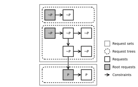
Inside a request set, the requests and their constraints form multiple trees. Indeed, requests which are unconstrained or whose constraints are outside the request set are the roots of distinct trees, while COALLOC or NEXT constraints determine parent-child relations (see Figure 12). Some of the algorithms that we shall present require navigating the request sets as a tree. Therefore, we define the following functions:

• roots : R7→ Rroots, returns the set of root requests in R

i.e., roots(R) ={r ∈ R, such that r.relatedHow = FREE ∨ r.relatedTo /∈ R}

• children : r, R7→ Rchildren, returns the set of child requests of r which belong to R i.e., children(r, R) ={rc∈ R, such that rc.relatedTo = r}

Figure 12: Example of request trees.

A.3 Views

Views (as defined in Section 3.1.4) map a cluster ID cid to a Cluster Availability Profile (CAP), which is a step function: the x-axis represents the absolute time, while the y-axis represents the number of available nodes. The CAPs are stores as a list of duration, node-count pairs. For example,

V ={a : [(3600, 4), (3600, 3)], b : [(∞, 6)]}

represents that on cluster a, 4 nodes are available for time t∈ [0, 3600), 3 nodes are available for time

t ∈ [3600, 7200) seconds and 0 nodes are available for time t ∈ [7200, ∞). On cluster b, 6 nodes are

always available.

Let us define a few operations on views:

• we note V [cid] the step-function which corresponds to cid in the view V ; e.g., for the view above, V [a] = [(3600, 4), (3600, 3)];

• cap : t7→ n, returns the number of nodes n available at time t;

e.g., V [a](1800) = 4, V [a](3600) = 3, V [a](7200) = 0;

• ∪ : V1, V27→ VR, returns the union view V of the views V1and V2;

i.e., V1∪ V2= V ⇔ V [cid](t) = max(V1[cid](t), V2[cid](t)),∀cid, t • + : V1, V27→ VR, returns the sum view V of the views V1 and V2;

i.e., V1+ V2= V ⇔ V [cid](t) = V1[cid](t) + V2[cid](t),∀cid, t

• − : V1, V27→ VR, returns the difference view V of the views V1and V2;

i.e., V1− V2= V ⇔ V [cid](t) = V1[cid](t)− V2[cid](t),∀cid, t

• alloc : V, r7→ n, returns the node-count that should be allocated to r, without changing its

start-time, limited by the resources available in V . This function is used to compute nalloc. i.e., alloc(V, r) = n⇔ n = min(mint_{∈[r.scheduledAt,r.scheduledAt+r.duration)}V [r.cid](t), r.n)

• findHole : V, r, t07→ ts, returns the first time after max(t0, r.earliestScheduleAt) when r could be started, so that all requested resources can be allocated;

i.e., find ts≥ max(t0, r.earliestScheduleAt), such that mint∈[ts,ts+r.duration)V [r.cid](t)≥ r.n

All above operations can be easily implemented by iterating through the list of duration, node-count pairs of the relevant CAPs. Due to their simplicity, the pseudo-code of the above operations is not given.

A.4

Helper Functions

In order to ease the description of the main scheduling algorithm, three helper functions are defined. Their purpose is to transform a set of requests into a view (called the generated view), representing how

resources are being occupied by the input requests. Once a set of requests has been transformed into generated views, the above defined operations on views can be used to compute the resources that are left unused after a set of requests is served. The helper functions are: toView, fit and eqSchedule. A.4.1 toView()

Algorithm 1: Implementation of the toView() function Input: R, set of requests

Vi, view of available resources (optional)

Output: Vo, view generated by requests

The scheduledAt, nalloc and fixed attributes of requests are updated

/* Initialization: start with an empty output view, clear fixed flag of requests

and create an empty queue */

1 Vo← ∅ ;

2 forall the r∈ R do r.fixed ← false ;

3 Q← ∅ /* Queue of requests which are to be processed */

/* First, add started requests to queue */

4 forall the r∈ R, such that started(r) do 5 enqueue(Q, r) ;

/* Next, process requests in the queue */

6 while Q6= ∅ do 7 r =dequeue(Q) ; 8 switch r.relatedHow do 9 case FREE 10 r.scheduledAt← r.startedAt ; 11 case NEXT

12 r.scheduledAt← r.relatedTo.scheduledAt + r.relatedTo.duration ;

13 case COALLOC

14 r.scheduledAt← r.relatedTo.scheduledAt ;

15 otherwise

16 continue /* Constraint not implemented */

17 if Vi =∅ then

18 r.nalloc= r.n ;

19 else

20 r.nalloc=alloc(Vi, r) ;

21 r.fixed← T rue ;

22 Vo← Vo+{r.cid : [(r.scheduledAt, 0), (r.duration, r.nalloc)]} ;

/* Enqueue children of this request */

23 forall the r_c∈ children(r) do 24 enqueue(Q, r) ;

toView() (see Algorithm 1) generates a view representing resources occupied by fixed requests, defined as requests which are either started or are constrained to a fixed request. These requests are treated specially, because the RMS cannot choose a start-time for them anymore. Indeed, in order not to violate the CooRMv2 protocol and allocate resources to applications according to their requests, the start-times are fixed. As a side effect, toView() sets the scheduledAt, fixed and nallocattributes of the input requests as needed.

For generating the view of preemptible requests, toView() accepts an optional parameter Vi

repre-senting the available resources. If this parameter is given, the generated view uses at most as many resources as available in Vi. The attribute nallocof preemptible requests is set according to this limit.

A.4.2 fit()

fit() (see Algorithm 2) generates a view representing resources that are occupied by non-fixed requests. The RMS has the liberty to choose the start-time for these requests, subject to the application-provided constraints.

The main idea of the algorithm is as follows. Each request has an earliestScheduleAt attribute, which specifies which is the time that the request can be scheduled the earliest. Initially, this attribute is set to t0, which is input to the algorithm (line 3). Then, the algorithm uses a queue of requests it has to process, which is initially filled with all root requests (line 5). Each request is then dequeue (line 7) and, depending on the request’s constraint, the scheduledAt attribute is computed (lines 14–33). If this attribute is changed, all child requests are queue, so as to recompute their scheduledAt attribute (lines 34–35).

In certain cases, the current schedule of the parent request makes it impossible for a child request to be scheduled so as to respect its constraint (lines 22, 31). If this happens, the earliestScheduleAt attribute of the parent is updated and the parent is added anew to the queue. This attribute is then used by findHole to find a later schedule-time for the parent, which might allow the child to find a valid schedule (lines 15, 21, 30). For preemptible requests, instead of delaying their parent, these requests are shrunken and nalloc is set accordingly (lines 19, 28). This behavior is allowed by the CooRMv2 specifications.

Eventually, the algorithm converges and the scheduledAt attribute of all requests is stable (in worst case, all requests are scheduled at infinity). The scheduledAt and nalloc attributes of the requests are used to computed the generated view (lines 36–38).

A.4.3 eqSchedule()

The purpose of this function is to do the equi-partitioning of resources available for preemptible requests. It gets as input the preemptible request set of each application, the view representing the available resources for equi-partitioning and the time after which non-started requests have to be scheduled. It outputs for each application a preemptible view. As a side effect, the scheduledAt and nallocattributes of requests are updated.

The pseudo-code is shown in Algorithm 3. It consists of three main parts. First, preliminary occu-pation views are computed (lines 1–3). These are used to determine time intervals, during which the requested node-count of all applications are constant. Second, for each piece-wise constant resource state (i.e., application resource request and available resources), the number of nodes that can be assigned to each application is determined (lines 4–27). Third, the computed views are used to reschedule the application requests and correctly set the scheduledAt and nalloc attributes of requests (lines 28–30).

The second part of the algorithm, which operates on a piece-wise constant resource state, works as follows. The system is either in a congested state, i.e., more resources are requested than are available for equi-partitioning, or the system is uncongested. The former situation might occur, due to the following reasons:

• since the last scheduling iteration, the number of resources for equi-partitioning has been reduced, • a new application has chosen to participate in equi-partitioning,

• an application has decided to increase the requested node-count and use more of its partition. If any of these situations occur, it is the duty of the RMS to inform malleable applications (by sending them new views), that they have to release some resources. The available resources are distributed equally, until the requests of applications are satisfied (lines 8–18).

In case the system is not congested (during a certain time interval), each application is assigned a view based on the number of resources that other applications leave unused (lines 19–25). However, this should not be smaller that the equi-partition of the application.

The number of equi-partitions is computed as follows (lines 22–23). Applications are either considered active, i.e., they currently request preemptible resources, or inactive. When computing the view of active applications, the number of partitions is equal to the number of active applications in the system. For inactive applications, the number of partitions is equal to the number of active applications in the system plus 1, i.e., the number of partitions if this application were to become active.

Algorithm 2: Implementation of the fit function

Input: R, set of requests (scheduledAt and fixed must have been set)

Vi, view of available resources

t0, requests have to be scheduled after this time Output: Vo, view generated by requests

The scheduledAt and nalloc attributes of non-fixed requests are updated

/* Initialization */

1 Q← ∅ /* Queue of requests which are to be processed */

2 forall the r∈ R, such that ¬r.fixed do

3 r.earliestScheduleAt← t0; /* No request can be scheduled earlier than t0 */

4 r.scheduledAt← ∞ ; /* In case of error, the request never starts */

/* First, add root requests to queue */

5 forall the r∈ roots(R) do enqueue(Q, r) ;

/* Next, deal with each request */

6 while Q6= ∅ do

7 r← dequeue(Q) ;

8 if r.fixed then /* If this is a fixed request, just add children to queue */ 9 forall the rc∈ children(r) do enqueue(Q, rc) ;

10 continue ;

/* Take a decision for the current request, depending on its constraint */

11 rp← r.relatedTo ; /* Store parent request to make pseudo-code briefer */

12 r.nalloc← r.n ; /* Set a default value for nalloc (will be overwritten later) */

13 tbefore← r.scheduledAt ; /* Store the previous value, used to detect changes */

14 switch r.relatedHow do

15 case FREE r.scheduledAt = findHole(V_i, r, 0) ;

16 case COALLOC

17 if r.type = P∧ rp.type∈ {P A, ¬P } then

18 r.scheduledAt← rp.scheduledAt ;

19 r.nalloc=alloc(Vi, r) ;

20 else

21 r.scheduledAt = findHole(Vi, r, rp.scheduledAt) ;

22 if r.scheduledAt6= r_p.scheduledAt then

23 rp.earliestScheduleAt← r.scheduledAt ;

24 enqueue(Q, r_p) ;

25 case NEXT

26 if r.type = P then

27 r.scheduledAt← rp.scheduledAt + rp.duration ;

28 r.nalloc=alloc(Vi, r) ;

29 else

30 r.scheduledAt = findHole(Vi, r, rp.scheduledAt + rp.duration) ;

31 if r.scheduledAt6= rp.scheduledAt + rp.duration then

32 rp.earliestScheduleAt← r.scheduledAt − rp.duration ;

33 enqueue(Q, rp) ;

/* If scheduledAt has changed, reschedule children */

34 if tbefore6= r.scheduledAt then

35 forall the rc∈ children(r) do enqueue(Q, rc)

/* Schedule converged, compute generated view */

36 Vo=∅ ;

37 forall the r∈ R, such that ¬r.fixed do