HAL Id: hal-02945065
https://hal.inria.fr/hal-02945065
Submitted on 26 Oct 2020
HAL is a multi-disciplinary open access
archive for the deposit and dissemination of
sci-entific research documents, whether they are
pub-lished or not. The documents may come from
teaching and research institutions in France or
abroad, or from public or private research centers.
L’archive ouverte pluridisciplinaire HAL, est
destinée au dépôt et à la diffusion de documents
scientifiques de niveau recherche, publiés ou non,
émanant des établissements d’enseignement et de
recherche français ou étrangers, des laboratoires
publics ou privés.
Connectivity Table
Hamid Boukerrou, Paul Huynh, Virginie Lallemand, Bimal Mandal, Marine
Minier
To cite this version:
Hamid Boukerrou, Paul Huynh, Virginie Lallemand, Bimal Mandal, Marine Minier. On the
Feis-tel Counterpart of the Boomerang Connectivity Table: Introduction and Analysis of the FBCT.
IACR Transactions on Symmetric Cryptology, Ruhr Universität Bochum, 2020, 2020 (1), pp.331-362.
�10.13154/tosc.v2020.i1.331-362�. �hal-02945065�
On the Feistel Counterpart of the Boomerang
Connectivity Table
Introduction and Analysis of the FBCT
Hamid Boukerrou, Paul Huynh, Virginie Lallemand, Bimal Mandal and
Marine Minier
Université de Lorraine, CNRS, Inria, LORIA, F-54000 Nancy, Francefirstname.name@loria.fr
Abstract. At Eurocrypt 2018, Cid et al. introduced the Boomerang Connectivity
Table (BCT), a tool to compute the probability of the middle round of a boomerang distinguisher from the description of the cipher’s Sbox(es). Their new table and the following works led to a refined understanding of boomerangs, and resulted in a series of improved attacks. Still, these works only addressed the case of Substitution Permutation Networks, and completely left out the case of ciphers following a Feistel construction. In this article, we address this lack by introducing the FBCT, the Feistel counterpart of the BCT. We show that the coefficient at row ∆i, ∇o corresponds to
the number of times the second order derivative at points (∆i, ∇o) cancels out. We
explore the properties of the FBCT and compare it to what is known on the BCT. Taking matters further, we show how to compute the probability of a boomerang switch over multiple rounds with a generic formula.
Keywords: Cryptanalysis · Feistel cipher · Boomerang attack · Boomerang switch
1
Introduction
Boomerang attacks date back to 1999, when David Wagner introduced them at FSE to break COCONUT98 [Wag99]. When presented, this variant of differential attacks [BS91] shook up the conventional thinking that consisted in believing that a cipher with only small probability differentials is secure. Indeed, boomerang attacks make use of two small differentials covering half of the attacked rounds each, and can beat differential cryptanalysis when no high probability differential exists for the whole cipher.
In the basic form of the distinguisher, (represented on the left in Figure1), the attacker has access to the encryption (E) and decryption (E−1) oracles, and studies particular quartets of messages. First, she chooses M1 and constructs M2= M1⊕ α; using E, she obtains the corresponding ciphertexts C1 and C2from which she deduces two additional ciphertexts by computing: C3= C1⊕ δ and C4= C2⊕ δ. By calling the decryption oracle
she retrieves the corresponding plaintexts M3 and M4 and then checks if M3⊕ M4= α.
A boomerang distinguisher is obtained if the probability that M3⊕ M4= α is higher for
the cipher than for a random permutation.
In summary, a boomerang distinguisher is based on a couple of plaintext and ciphertext differences (α, δ) for which the following property among quartets of messages has a high probability:
E−1(E(M1) ⊕ δ) ⊕ E−1(E(M1⊕ α) ⊕ δ) = α.
In the original approach, the attacked cipher E is written as the composition of two sub-ciphers E0 and E1: E = E1◦ E0. If for the sub-cipher E0the input difference α leads
Licensed underCreative Commons License CC-BY 4.0.
to the output difference β with probability p (and similarly γ leads to δ with probability q over E1) the previous event was thought to have a probability of p2q2.
Following this breakthrough some variants were proposed including a related-key version [KKH+04,BDK05] and an impossible-differential one (see [CY09]). Improvements
were also proposed on top of this, like a version that does not require access to the decryption oracle (named amplified boomerang attack [KKS01]) that was further developed into the so-called rectangle attack [BDK01].
The validity of boomerang attacks and in particular of the p2q2 formula were later
questioned by Murphy [Mur11] with an example of distinguisher that seemed valid but
was in fact of probability zero. The opposite phenomenon, that is distinguishers that happen with probability higher than what is expected, was also presented by Biryukov and Khovratovich in [BK09], and some particular cases (termed Ladder Switch, Sbox Switch and Feistel Switch) were explained.
All these observations were later formalized in a framework called sandwich
at-tack [DKS10] for which the cipher is divided in 3 parts instead of 2, as represented
on the right of Figure 1: a middle part Em (termed boomerang switch) is introduced
between E0 and E1. Dunkelman et al. applied this framework to KASUMI.
M1 E0 E1 C1 M2 E0 E1 C2 α β M3 E0 E1 C3 M4 E0 E1 C4 α β γ γ δ δ 1 2 3 4 M1 E0 Em C1 M2 E0 E1 C2 α β M3 E0 C3 M4 E0 C4 α β γ x1 x2 x3 x4 Em Em Em y1 y2 y3 y4 E1 E1 E1 γ δ δ 1 2 3 4
Figure 1: Configuration of the basic boomerang attack (left) and of the sandwich attack (right). Circled numbers correspond to a numbering that helps referencing states in the following discussions.
Cid et al. [CHP+18] recently introduced a tool called the Boomerang Connectivity
Table that allows to easily evaluate the probability of the middle part Emin the case where
it covers one round and when the studied ciphers follows an SPN construction. Their technique reduces the problem of computing the probability of the boomerang switch over one round function to the one of computing it over one Sbox only.
Equally as an Sbox with a Difference Distribution Table with small coefficients provides resistance against differential attacks, an Sbox with a Boomerang Connectivity Table (BCT) with small coefficients prevents an attacker from building efficient boomerang-style attacks. A study of some important families of Sboxes has been made in [BC18], [BPT19] and [LQSL19], just to cite a few. Another interesting line of work that followed the paper of Cid et al. is the determination of the probability of a boomerang switch Emthat covers more than one round, and that was addressed for SPN ciphers in [WP19,SQH19].
Still, to the best of our knowledge a similar analysis has not been provided yet for Feistel constructions [Fei74], while it cannot be denied that it is an equally important type of block cipher design, instantiated for instance by the widely used 3-DES and by CLEFIA [SSA+07] (ISO/IEC 29192-2).
Our Contributions. In this work, we address this lack and investigate what can be said on a boomerang switch when the studied cipher follows a Feistel construction. In case the Feistel round function contains some affine layers and a single Sbox layer we introduce the FBCT, the Feistel counterpart of the Boomerang Connectivity Table and show that it is related to the second order derivative of the Sbox at play. Our model elucidates the last switch that is not explained by the BCT by showing that the Feistel Switch corresponds to the diagonal of our table.
We study the properties of the FBCT for some categories of cryptographic Sboxes (in particular APN Sboxes and Sboxes based on the inverse mapping) and investigate if the maximum in the FBCT is invariant for Sboxes that are in the same equivalence classes for an equivalence that is affine, extended-affine and CCZ.
In a bottom-up approach, we start from this notion of FBCT (that covers switches of one round) and then introduce the FBDT to deal with a 2-round switch and finally propose the FBET that treats the case of an arbitrary number of rounds. We explain the relation between all these new notions and give examples of their application.
Finally, we illustrate our approach by applying it to the cipher LBlock-s (used in the CAESAR candidate LAC), and provide a 16-round distinguisher which probability is evaluated to be higher than 2−56.14.
2
Motivation: Disproving the Validity of a Previous
Boo-merang Distinguisher on LBlock
As a warm up, we study the related-key boomerang distinguisher devised by Liu et al. on LBlock [LGW12] and prove that the middle part contains a contradiction that invalidates the proposed boomerang distinguisher.
2.1
Specification of LBlock
LBlock was proposed at ACNS 2011 [WZ11] by Wenling Wu and Lei Zhang. The cipher
is lightweight and works on blocks of 64 bits and requires a key of 80 bits. It follows a Feistel structure and has the particularity to rely on 10 different 4-bit Sboxes. We give a short description of its design below and refer to [WZ11] for more details and in particular for the description of the key schedule.
One LBlock encryption requires to iterate 32 times a round function that follows a 2-branch balanced Feistel structure with a twist, that is the right branch is modified by a rotation of 8 bit positions (see Figure2). The other half of the internal state is modified by the F function that takes as parameter the 32-bit round key Ki. If the plaintext is denoted M = X1||X0(where || denotes the concatenation), we have for all 33 ≥ i ≥ 2:
Xi= F (Xi−1, Ki−1) ⊕ (Xi−2≪ 8). More into details, the function F is defined as:
F : {0, 1}32× {0, 1}32 → {0, 1}32
(X, Ki) → U = P (S(X ⊕ Ki)).
S is an Sbox layer that transforms each nibble Yi into the nibble Zi= Si(Yi):
S : {0, 1}32 → {0, 1}32
Y7||Y6||Y5||Y4||Y3||Y2||Y1||Y0 → Z7||Z6||Z5||Z4||Z3||Z2||Z1||Z0, Zi= Si(Yi). The Sboxes are detailed in Table5in AppendixA. P is a permutation given by:
P : {0, 1}32 → {0, 1}32
F <<< 8 Xi−1 Xi−2 Xi Xi−1 Ki−1 Ki S7 S6 S5 S4 S3 S2 S1 S0 X
Figure 2: High-level description of one round of LBlock (left) and description of the F function (right).
2.2
Attack of Liu et al.
In 2012, Liu et al. [LGW12] proposed a 16-round related-key boomerang distinguishing attack on LBlock based on two 8-round related-key characteristics of low weight (that is, with very few active Sboxes). This attack is supposed to work in some (very large) weak-key class as it includes a key condition. With their parameters (that we recall in Appendix B), the probability of E0 is p = 2−14, while the probability of E1is q = 2−16.
They next computed the probability of the obtained distinguisher with the approximation
p2q2, that gives 2−60. Unfortunately, next section details why the two characteristics E0
and E1 are in fact incompatible, meaning that the actual probability that the boomerang
returns along these differential characteristics is 0.
2.3
Incompatibility in the Distinguisher Proposed by Liu et al.
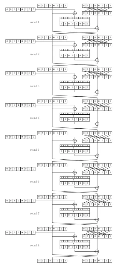
To help visualize the following discussion, we provide in Figure3a representation of the end of E0 and of the beginning of E1. In the following, we assume that the required
transition happened in the key schedule (that is 0x3 →S9 0x8 in round 7).
0 0 0 0 0 0 0 0 round 8 of E0 S S S S S S S S round 9 of E0 S S S S S S S S 0 0 0 0 0 2 0 0 round 1 of E1 S S S S S S S S 0 0 0 0 2 0 0 0 0 0 0 0 4 9 0 0 0 0 0 0 4 9 0 0 0 8 0 0 0 0 5 8 0 0 0 0 5 0 0 0 0 0 0 0 1 8 0 0 0 0 0 1 0 0 8 8 0 0 0 1 5 0 a 8 0 0 0 1 5 0 8 0 0 0 0 0 4 9 0 0 0 0 0 0 0 0 2 0 0 0 4 9 0 0 0
(extended with probability 1)
2 0 0 0 0 0 0 0 0 0 0 0 0 0 0 0 0 0 0 0 0 0 2 0 0 0 0 0 0 0 2 0 0 0 0 0 0 2 0 0 0 0 0 0 0 0 0 0 0 0 0 0 0 0 0 0 0 8 0 0 0 1 5 0 8
difference between and1 and between3 and2 4
X9 X8 X9 X8
difference between and1 and between2 and3 4
K9 K9
Figure 3: Middle rounds of the boomerang distinguisher proposed in [LGW12].
Suppose that the quartet (M1, M2, M3, M4) follows the characteristics defining the boomerang specified by Liu et al. When looking at the beginning of the characteristic
of 0x2 to 0x2, while by extending with probability 1 the differential characteristic over
E0 we see that the entering difference for this same Sbox is 0x5 (see Figure 3). If we
denote by ti the nibble that enters the Sbox number 2 of round 9 for Mi, this means that t1⊕ t3= t2⊕ t4=0x2 and that S
2(t1) ⊕ S2(t3) = S2(t2) ⊕ S2(t4) =0x2. Also, we have
t1⊕ t2= t3⊕ t4=0x5.
By referring to S2, we can list the possible input nibbles that make the transition
from an input difference of 0x2 to an output difference of 0x2, and we obtain that (t1, t3) ∈ {(0x1,0x3), (0x3,0x1), (0x8,0xa), (0xa,0x8)}. Since t2 and t4 are separated from
t1and t3 by a difference of 0x5 we can deduce that their values are in the following set:
(t2, t4) ∈ {(0x4,0x6), (0x6,0x4), (0xd,0xf), (0xf,0xd)}.
The contradiction comes from the fact that none of these pairs allows the required transition from 0x2 to 0x2, an observation that can be rewritten as: {(0x1, 0x3), (0x3, 0x1), (0x8, 0xa), (0xa, 0x8)} ∩ 0x5 ⊕ {(0x1, 0x3), (0x3, 0x1), (0x8, 0xa), (0xa, 0x8)} = ∅ since we want that the shifted values (t1, t3) also allows the desired Sbox transition.
This incompatibility implies that the boomerang over the middle round never returns,1 and consequently the related-key distinguisher proposed by Liu et al. is invalid as no quartet can follow the required characteristic.
3
FBCT: the Feistel Counterpart of the BCT
The inconsistency found in the previous section (that is reminiscent of the examples given by Murphy in [Mur11]) calls for a tool to automatically study the behavior of the junction between E0 and E1.
In fact, this problem has recently been addressed in the case of Substitution-Permutation Networks with the introduction of the Boomerang Connectivity Table (BCT) by Cid et al [CHP+18]. However, no similar tool has been devised so far to deal with boomerang attacks on Feistel Networks. We address this shortfall in this section by introducing the2 FBCT.
3.1
Definition of the FBCT
The (SPN) Boomerang Connectivity Table. The essence of the Boomerang Connectivity
Table introduced by Cid et al. is similar to the one of the well-known Difference Distribution Table: instead of looking at the property of a round as a whole (thus at a function of usually 64 or 128 bits), the problem is reduced to one we can easily study given its small size: examining each Sbox of the S-layer independently. While the DDT describes the differential properties of each Sbox from which are deduced the ones of the round, the BCT gives the probability of a boomerang switch over each Sbox from which is deduced the one of the round.
The formal definition of the BCT is recalled below: it is a table that gives at line ∆i, column ∇othe number of values for which a boomerang of input ∆i and output difference ∇ocomes back. It corresponds to the following formula, depicted in Figure 4:
Definition 1 (Boomerang Connectivity Table [CHP+18
]). Let S be a permutation of Fn
2,
and ∆i, ∇o∈ Fn2. The Boomerang Connectivity Table (BCT) of S is given by a 2
n× 2n table, in which the entry for the (∆i, ∇o) position is given by:
BCT (∆i, ∇o) = #{x ∈ Fn2|S
−1(S(x) ⊕ ∇
o) ⊕ S−1(S(x ⊕ ∆i) ⊕ ∇o) = ∆i}.
1Note that we confirmed this experimentally by verifying that for a sample of 210keys and 210messages the boomerang never comes back along the announced differences in one or even two middle rounds.
2To stress the similarity between the notions we introduce here and the ones that have been previously introduced in the case of boomerang switches on SPN, we basically use the same acronyms, simply adding the letter "F" in front of them to recall that we are looking at the Feistel case.
x S S(x) ∆i ∇o S S(x⊕ ∆i) S S ∇o ∆i? S(x⊕ ∆i)⊕ ∇o S(x)⊕ ∇o
Figure 4: The value of BCT (∆i, ∇o) corresponds to the number of Sbox inputs x that
make the boomerang over 1 round come back.
The Feistel Boomerang Connectivity Table. The previous definition is only valid for an
Sbox that is part of an S-layer in an SPN cipher: the objective of this paper is to address the need of the counterpart for a Feistel cipher.
As a hint of what we introduce below, remember that Feistel ciphers have the practical advantage that decryption is performed by executing the same function as for encryption, simply changing the order of the round keys. This change is at the heart of the Feistel counterpart of the BCT that we introduce now: here, the inverse of the Sbox is never at play.
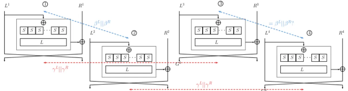
We start by illustrating our theory on the generic Feistel3cipher represented in Figure5: it is a balanced Feistel with two branches, that we denote L and R. The output of one round is given by F (L) ⊕ R||L, where the F function is defined by a round key addition, an S-layer and a linear layer L. Note that the details of the linear layers of F play no role in our discussion, and that the only important point is that F contains one S-layer made by the concatenation of t n-bit Sboxes.
βL||βR γL||γR = βL||βR? γL||γR L1 R1 L2 R2 L3 R3 R4 L4 G3 G4 S L S S S S S L S S S S S L S S S S S L S S S S · · · · · · · · · · · · 1 2 3 4
Figure 5: Boomerang switch over a generic Feistel round.
We are interested in the probability of the following 1-round boomerang switch: we have an input difference equal to βL||βR between state and1 , an output difference2 equal to γL||γR between state and1 , and3 and2 , and we want that the input4 difference between state and3 is equal to β4 L||βR.
Left part of the difference. We start by studying the cost of obtaining that the left
difference between state and3 has the desired value of β4 L.
Given the fact that the left branch is the one that is not modified through one round of Feistel we can easily conclude that the desired difference comes for free:
L3⊕ L4 = (L3⊕ L1) ⊕ (L1⊕ L2) ⊕ (L2⊕ L4)
= γR⊕ βL⊕ γR= βL.
Right part of the difference. We now focus on obtaining a difference of βR between the right part of state number and3 . By naming G4 3 and G4 the left output after one
round in state and3 (see Figure4 5), we obtain the following simplification:
R3⊕ R4 = F (L1⊕ γR) ⊕ G3⊕ F (L1⊕ γR⊕ βL) ⊕ G4
= F (L1⊕ γR) ⊕ F (L1) ⊕ R1⊕ γL⊕ F (L1⊕ γR⊕ βL) ⊕F (L1⊕ βL) ⊕ R1⊕ βR⊕ γL
= F (L1⊕ γR) ⊕ F (L1) ⊕ F (L1⊕ γR⊕ βL) ⊕F (L1⊕ βL) ⊕ βR.
For this difference to be equal to βRwe need that
F (L1) ⊕ F (L1⊕ γR) ⊕ F (L1⊕ βL) ⊕ F (L1⊕ γR⊕ βL) = 0.
We use the fact that the only non-linear function of F is an S-layer made by a concatenation of small Sboxes to rewrite this condition as a set of independent conditions on smaller parts of the states, and obtain t independent equations of the form:
S(x) ⊕ S(x ⊕ ∆i) ⊕ S(x ⊕ ∇o) ⊕ S(x ⊕ ∆i⊕ ∇o) = 0.
Where ∆iis the difference at the input of the considered Sbox between state and1 2
, deduced from βL, and ∇
ois the difference at the input of the considered Sbox between state and1 and3 and2 , deduced from γ4 R.
The resulting probability of the boomerang switch over one round is then the product of the probabilities for each Sbox, that are of the form
2−n× #{x ∈ Fn
2|S(x) ⊕ S(x ⊕ ∆i) ⊕ S(x ⊕ ∇o) ⊕ S(x ⊕ ∆i⊕ ∇o) = 0}. This discussion leads us to the introduction of the following definition:
Definition 2 (FBCT). Let S be a function from Fn
2 to Fm2 , and ∆i, ∇o ∈ Fn2. The FBCT
of S is given by a 2n× 2n table T , in which the entry for the (∆
i, ∇o) position is given by: FBCTS(∆i, ∇o) = #{x ∈ Fn2|S(x) ⊕ S(x ⊕ ∆i) ⊕ S(x ⊕ ∇o) ⊕ S(x ⊕ ∆i⊕ ∇o) = 0}.
Since we do not have to consider a bijective Sbox, we define FBCTS for any Sbox S from Fn
2 to Fm2 with possibly n 6= m. In the following we leave out the S index and simply
write FBCT when the Sbox we are referring to is clear from the context.
Once the table is built, the probability that a boomerang comes back over 1 round of a Feistel scheme is simply the product of the corresponding coefficients of the FBCT divided by 2n. An example of FBCT is provided in Table1in the case of the Sbox4S2 of LBlock.
It is easy to see that the formula of the FBCT corresponds to the number of times the order 2 derivative with respect to ∆i and ∇o of the vectorial Boolean function S cancels out. We formalize this and study its properties in Section4.
3.2
Evaluation of the 1-round Boomerang Switch of Liu et al.’s Attack
with the FBCT
We focus on the Sbox S2 of round 9 of the cipher. From E0, the input difference of Sbox
2 is 0x5, so following previous notation we have ∆i = 0x5. When referring to E1 and
taking into account the difference coming from the round key we have ∇o = 0x2. The
4
Note that the FBCT of the 10 Sboxes of LBlock are the same. This is not a direct implication of the fact that the Sboxes are affine equivalent (counter-examples to this can easily be found).
Table 1: FBCT of the Sbox S2of LBlock. 0 1 2 3 4 5 6 7 8 9 a b c d e f 0 16 16 16 16 16 16 16 16 16 16 16 16 16 16 16 16 1 16 16 0 0 0 0 0 0 0 0 8 8 0 0 0 0 2 16 0 16 0 0 0 0 0 0 8 0 8 0 0 0 0 3 16 0 0 16 8 8 8 8 0 0 0 0 0 0 0 0 4 16 0 0 8 16 0 0 8 0 0 0 0 0 0 0 0 5 16 0 0 8 0 16 8 0 0 0 0 0 0 0 0 0 6 16 0 0 8 0 8 16 0 0 0 0 0 0 0 0 0 7 16 0 0 8 8 0 0 16 0 0 0 0 0 0 0 0 8 16 0 0 0 0 0 0 0 16 0 0 0 0 0 0 0 9 16 0 8 0 0 0 0 0 0 16 0 8 0 0 0 0 a 16 8 0 0 0 0 0 0 0 0 16 8 0 0 0 0 b 16 8 8 0 0 0 0 0 0 8 8 16 0 0 0 0 c 16 0 0 0 0 0 0 0 0 0 0 0 16 0 0 0 d 16 0 0 0 0 0 0 0 0 0 0 0 0 16 0 0 e 16 0 0 0 0 0 0 0 0 0 0 0 0 0 16 0 f 16 0 0 0 0 0 0 0 0 0 0 0 0 0 0 16
FBCT coefficient we are interested in is then FBCTS2(0x5, 0x2). Referring to Table1, we see that the corresponding cell has a value equal to 0, meaning that the 1-round boomerang switch is impossible.
Note that this incompatibility is even more general than the one we discussed in
Sec-tion 2.3, as in Section 2.3 we fixed an additional parameter namely one Sbox output.
This vision corresponds to what we introduce in Section5.1 under the name of Feistel
Boomerang Difference Table (FBDT).
3.3
Relation Between the FBCT and the Feistel Switch
While the Feistel case is not covered by the Boomerang Connectivity Table, a first step in understanding the case of boomerang distinguishers for Feistel constructions has been made
by Wagner himself while analyzing Khufu [Wag99]. His observation was later referred
under the name of Feistel Switch, for instance in the related-key cryptanalysis of the
AES-192 and AES-256 by Biryukov and Khovratovich [BK09], in which one can read:
Surprisingly, a Feistel round with an arbitrary function (e.g., an S-box) can be passed for free in the boomerang attack (this was first observed in the attack on cipher Khufu in [Wag99]). Suppose the internal state (X, Y ) is transformed to (Z = X ⊕ f (Y ), Y ) at the end of E0. Suppose also that the E0 difference
before this transformation is (∆X, ∆Y ), and that the E1difference after this
transformation is (∆Z, ∆Y ). [. . .] Therefore, the decryption phase of the boomerang creates the difference ∆X in X at the end of E0“for free”.
By analyzing this setting in the way we did in Section3.1we can show that an internal state (X, Y ) allows the boomerang to come back if Y verifies:
f (Y ) ⊕ f (Y ⊕ ∆Y ) ⊕ f (Y ⊕ ∆Y ) ⊕ f (Y ⊕ ∆Y ⊕ ∆Y ) = 0,
(we have γR= βL = ∆Y with our previous notation) which is always true. Moreover if the Feistel round function is made of some linear operations and an S-layer, the previous setting means that for every Sbox we are looking at coefficients that are on the diagonal of the FBCT.
4
Properties of the FBCT
This section gives a review of the most important properties of the Feistel boomerang connectivity table. We start by listing the constants of the table and then investigate the properties of the FBCT of two crucial classes of vectorial function, namely APN functions and functions based on the inverse mapping. We also study if the so-called Feistel boomerang uniformity is constant for Sboxes belonging to the same equivalence classes, for various definitions of equivalence. We conclude this section by giving a comparison of the BCT and FBCT properties.
4.1
Basics on vectorial Boolean Functions
Let S : Fn2 −→ Fm2 be a vectorial Boolean function. The set of all vectorial Boolean
functions from Fn
2 to Fm2 is denoted B(n, m). The derivative of S ∈ B(n, m) at ∆i∈ Fn2 is
defined as
D∆iS(x) = S(x) ⊕ S(x ⊕ ∆i)
for all x ∈ Fn
2.
The first derivative is at the basis of the Difference Distribution Table (DDT) of a given vectorial function S, defined as:
DDTS(∆i, δ) = #{x ∈ Fn2 : S(x) ⊕ S(x ⊕ ∆i) = δ}.
The value of max∆i6=0,δ{DDTS(∆i, δ)} is called the (differential) uniformity of S. This definition is extended to higher-order derivatives as follows: let ∆1
i, ∆2i, . . . , ∆ k i be a basis of a k-dimensional subspace V of Fn2. The k-th derivative of S with respect to V ,
denoted by DVS, is defined as DVS(x) = D∆1 iD∆ 2 i· · · D∆kiS(x), for all x ∈ F n 2.
Given this definition, it is direct to see that for an n × m Sbox seen as an element of B(n, m), the value of FBCT(∆i, ∇o) corresponds to the number of zeroes of the function
D∆iD∇oS extended to the cases where ∆i and ∇o are not linearly independent.
4.2
Some Direct Properties of any FBCT
We start with a series of simple properties that are easily observable from the definition: Property 1. The coefficients of the FBCT of S ∈ B(n, m) verify the following:
1. Symmetry: for all 0 ≤ ∆i, ∇o≤ 2n− 1, FBCT(∆i, ∇o) = FBCT(∇o, ∆i). 2. Fixed values:
(a) First line: for all 0 ≤ ∇o≤ 2n− 1, FBCT(0, ∇o) = 2n (ladder switch), (b) First column: for all 0 ≤ ∆i≤ 2n− 1, FBCT(∆i, 0) = 2n (ladder switch),
(c) Diagonal: for all 0 ≤ ∆i≤ 2n− 1, FBCT(∆i, ∆i) = 2n (Feistel switch). 3. Multiplicity: for all 0 ≤ ∆i, ∇o≤ 2n− 1, FBCT(∆i, ∇o) ≡ 0 mod 4.
4. Equalities: for all 0 ≤ ∆i, ∇o≤ 2n− 1, FBCT(∆i, ∇o) = FBCT(∆i, ∆i⊕ ∇o).
Proof. All the properties are easily deduced from Definition 2:
(1) and (4) are proven by writing the expressions of the coefficients at play. Note that from symmetry we also have FBCT(∆i, ∆i⊕ ∇o) = FBCT(∇o, ∆i⊕ ∇o).
(2)a. and (2)b. correspond to the ladder switch proposed in [BK09] that works the same way for Feistel and SPN ciphers: if either ∆i or ∇o is zero, it means that two pairs
of messages inside the quartet share the same Sbox input, and the boomerang comes back with probability 1. This is formally shown as follows:
FBCT(0, ∇o) = #{x ∈ Fn2|S(x) ⊕ S(x) ⊕ S(x ⊕ ∇o) ⊕ S(x ⊕ ∇o) = 0} = 2n,
and similarly FBCT(∆i, 0) = 2n. The Feistel switch recalled in Section 3.3 is also easily proven: if ∆i = ∇o the FBCT coefficients correspond to the number of x ∈ Fn2 that are
solutions to S(x) ⊕ S(x ⊕ ∆i) ⊕ S(x ⊕ ∆i) ⊕ S(x) = 0. Since every value of x fulfills this, FBCT(∆i, ∆i) = 2n.
(3) The property is verified for the case ∆i = ∇o (since we can reasonably assume
n > 1), so we focus on the case where ∆i6= ∇o. If no x is solution the property is verified,
while if there is at least one x ∈ Fn
2 that is a solution then three more distinct values
x ⊕ ∆i, x ⊕ ∇o and x ⊕ ∆i⊕ ∇oalso are, which proves the multiplicity.
Given that the coefficients in the first line, first column and diagonal of the FBCT are always equal to the maximum that is 2n, we define the boomerang uniformity a bit differently from what has been done for the BCT5:
Definition 3 (F-Boomerang Uniformity). The F-Boomerang uniformity corresponds to
the highest value in the FBCT without considering the first row, the first column and the diagonal:
βF = max
∆i6=0,∇o6=0,∆i6=∇o.
FBCT(∆i, ∇o).
From the designer point of view, it is preferable to use an Sbox with a small F-boomerang uniformity. This goal can be reached by opting for an APN function, as we show below.
4.3
On the FBCT of APN Functions
A function S ∈ B(n, n) is called almost perfect nonlinear (APN) if for any ∆i, δ ∈ Fn2 with
∆i6= 0 the equation S(x) ⊕ S(x ⊕ ∆i) = δ has either 0 or 2 solutions. Alternatively, we know (refer for instance to [Car10], page 417) that S is APN if and only if for any non-zero ∆i, ∇o∈ Fn2 with ∆i 6= ∇o, D∆iD∇oS(x) 6= 0 for all x ∈ F
n
2. This directly implies the
following theorem:
Theorem 1. Let S ∈ B(n, n). S is an APN function if and only if its FBCT verifies
FBCT(∆i, ∇o) = 0 for all 1 ≤ ∆i6= ∇o≤ 2n− 1.
A direct implication of this theorem is that any non-APN function has a non-zero coefficient at a position that is not in the first row, first column or diagonal of its FBCT, so in particular a Feistel boomerang uniformity higher or equal to 4.
4.4
On the FBCT of Sboxes based on the Inverse Mapping
Another important and widely used set of Sboxes are the ones based on the inverse mapping, which include (among others) the 8-bit Sboxes of CAMELLIA [AIK+01], Clefia [SSA+07] and SMS4 [Dt08] and the 4-bit Sbox of Twine [SMMK13].
We know that Fn
2 and F2nare vector isomorphic over F2, i.e., with respect to a fixed basis
αi, 1 ≤ i ≤ n, of F2n, any element of x ∈ F2n can be uniquely written as x = ⊕ni=1xiαi,
where (x1, x2, . . . , xn) ∈ F2n. A mapping S : F2n→ F2n of the form S(x) = x2 n−2
is called an inverse mapping.
5Recall that for the BCT the boomerang uniformity of an Sbox is β = max
The importance of this family of functions comes from its very good cryptographic properties (that lead to it being selected to build the AES [AES01] Sbox for instance). Indeed, Nyberg [Nyb94] showed that if n is odd, then the inverse function over F2n is APN, and if n is even, then each row of its DDT has exactly one 4 and (2n−1− 2) occurrences of the number 2 (and in particular that the Sbox is differentially 4-uniform). Given that we already discussed the case of APN functions in Section4.3, we focus here on the case where n is even.
Property 2. In each row (except the first) of the FBCT of the inverse mapping over an even number of bits, the values 2n, 4 and 0 occur 2, 2 and 2n− 4 times, respectively. Proof. Using a reductio ad absurdum argument, we start by showing that the only possible
values in the FBCT of the inverse mapping over an even number of bits are 0, 4 and 2n. Since for every FBCT the coefficients in the first line, first column and diagonal are equal to 2n, we focus on the other positions.
Suppose that for given non-zero ∆iand ∇overifying ∆i6= ∇owe have FBCT(∆i, ∇o) > 4. Given that the coefficients of the FBCT are multiple of 4 this implies that we have at least 8 distinct values x, x ⊕ ∆i, x ⊕ ∇o, x ⊕ ∆i⊕ ∇o, y, y ⊕ ∆i, y ⊕ ∇o, y ⊕ ∆i⊕ ∇othat are solutions of:
S(x) ⊕ S(x ⊕ ∆i) ⊕ S(x ⊕ ∇o) ⊕ S(x ⊕ ∆i⊕ ∇o) = 0.
This can be rewritten as:
S(x) ⊕ S(x ⊕ ∆i) = S(x ⊕ ∇o) ⊕ S(x ⊕ ∆i⊕ ∇o) = δ1, (1)
S(y) ⊕ S(y ⊕ ∆i) = S(y ⊕ ∇o) ⊕ S(y ⊕ ∆i⊕ ∇o) = δ2. (2)
The first line indicates that the equation S(x) ⊕ S(x ⊕ ∆i) = δ1 has at least 4 distinct
solutions, that is DDT(∆i, δ1) ≥ 4. Similarly, the second line shows that DDT(∆i, δ2) ≥ 4.
There are two possibilities: if δ1 = δ2 we obtain that DDT(∆i, δ1) ≥ 8 which contradicts
that the differential uniformity of the considered Sbox is 4, while if δ16= δ2 we obtain that
there are two coefficients in the same line of the DDT with a coefficient higher or equal to 4. In both cases we obtain a contradiction, so we conclude that the only possible values in the FBCT are 0, 4 and 2n.
To conclude on the number of occurrences of each coefficient we need to prove that there are only 2 coefficients equal to 4 in each line. We consider ∆i, δ ∈ Fn2 so that
DDT(∆i, δ) = 4. There exist x, x ⊕ ∆i, y, y ⊕ ∆i∈ Fn2 with x 6= y and x 6= y ⊕ ∆i such that:
S(x) ⊕ S(x ⊕ ∆i) = δ = S(y) ⊕ S(y ⊕ ∆i)
i.e. S(x) ⊕ S(x ⊕ ∆i) ⊕ S(x ⊕ ∇o) ⊕ S(x ⊕ ∇o⊕ ∆i) = 0, where ∇o= x ⊕ y.
As a consequence, FBCT(∆i, ∇o) = FBCT(∆i, ∆i⊕ ∇o) = 4 so there are at least two ’4’ in each line of the FBCT. Suppose there is one more coefficient equal to 4 in this line, that is there exists c ∈ Fn
2 with c 6= ∇o and c 6= ∆i⊕ ∇o such that FBCT(∆i, c) = 4 and let
z ∈ {x ∈ Fn2|S(x) ⊕ S(x ⊕ ∆i) ⊕ S(x ⊕ c) ⊕ S(x ⊕ ∆i⊕ c) = 0}. We have:
S(z) ⊕ S(z ⊕ ∆i) ⊕ S(z ⊕ c) ⊕ S(z ⊕ ∆i⊕ c) = 0
i.e. S(z) ⊕ S(z ⊕ ∆i) = δ0 = S(w) ⊕ S(w ⊕ ∆i), where w = z ⊕ c.
FBCT(∆i, c) = 4 yields c 6= ∆i and c 6= 0 and thus DDT(∆i, δ0) = 4 = DDT(∆i, δ). Since each row of the considered Sbox DDT has exactly one entry that equals 4, it follows that
δ = δ0 and that z, w ∈ {x, x ⊕ ∆i, y, y ⊕ ∆i}, which leads to the contradiction that
4.5
On the FBCT of Equivalent Sboxes
Various notions of equivalence are frequently used when studying Sboxes, among which
linear, affine, extended-affine and CCZ equivalence [CCZ98]. These various concepts
play an important role to categorize sets of Sboxes since central cryptographic properties (differential, linear and sometimes algebraic degree) are constant for equivalent Sboxes. In this section we investigate if the F-boomerang uniformity is preserved under these various notions of equivalence.
Linear, Affine and Extended-Affine Equivalence. As their names suggest, the three
first flavors we start with are related as follows: linear equivalence is a sub-case of affine equivalence, and affine equivalence is a particular case of extended-affine equivalence. Definition 4 (Linear, Affine and Extended-Affine Equivalence). Two vectorial Boolean functions F, G ∈ B(n, m) are called extended-affine equivalent if there exist two nonsingular matrices A ∈ GL(n, F2), B ∈ GL(m, F2), (a, b) ∈ Fn2× Fm2 and an affine function C : Fn2 →
Fm2 such that for all x ∈ Fn2
G(x) = B(F (A(x) ⊕ a)) ⊕ C(x) ⊕ b,
where GL(n, F2) is the set of all nonsingular binary matrices of order n. If C = 0, then
F and G are affine equivalent, and if in addition a and b are equal to zero then they are
linear equivalent.
Theorem 2. The multi-set composed of all values in the FBCT is preserved under
extended-affine nonsingular transformation. Namely, we have that FBCTG(u, v) = FBCTF(u0, v0)
where u0= A(u) and v0= A(v).
Proof. Suppose that G(x) = B(F (A(x)⊕a))⊕C(x)⊕b for all x ∈ Fn
2, where A ∈ GL(n, F2),
B ∈ GL(m, F2), (a, b) ∈ Fn2 × F
m
2 and C ∈ B(n, m) is an affine function. Using the fact
that C(x) ⊕ C(x ⊕ u) ⊕ C(x ⊕ v) ⊕ C(x ⊕ u ⊕ v) = 0, for all x ∈ Fn2 and u, v ∈ F
n
2, we
obtain the following relations:
FBCTG(u, v) = #{x ∈ Fn2 : G(x) ⊕ G(x ⊕ u) ⊕ G(x ⊕ v) ⊕ G(x ⊕ u ⊕ v) = 0}
= #{x ∈ Fn2 : B(F (A(x) ⊕ a)) ⊕ B(F (A(x ⊕ u) ⊕ a)) ⊕ B(F (A(x ⊕ v) ⊕ a))
⊕ B(F (A(x ⊕ u ⊕ v) ⊕ a)) = 0}
= #{x ∈ Fn2 : B(F (A(x) ⊕ a) ⊕ F (A(x ⊕ u) ⊕ a) ⊕ F (A(x ⊕ v) ⊕ a)
⊕ F (A(x ⊕ u ⊕ v) ⊕ a)) = 0} = #{x ∈ Fn2 : F (A(x) ⊕ a) ⊕ F (A(x) ⊕ u 0⊕ a) ⊕ F (A(x) ⊕ v0⊕ a) ⊕ F (A(x) ⊕ u0⊕ v0⊕ a) = 0} = #{y ∈ Fn2 : F (y) ⊕ F (y ⊕ u0) ⊕ F (y ⊕ v0) ⊕ F (y ⊕ u0⊕ v0) = 0} = FBCTF(u0, v0),
where u0 = A(u), v0= A(v) and the new variable y corresponds to A(x) ⊕ a.
In particular, the F-boomerang uniformity is constant among Sboxes in the same linear, affine or extended-affine equivalence class.
CCZ Equivalence. The last equivalent relation we discuss here is the CCZ
equiva-lence [CCZ98]. Concluding on this case is rather easy: it is known that every permutation is CCZ-equivalent to its inverse, and we show in next subsection that Feistel boomerang uniformity is not necessarily the same for an Sbox and its inverse. Consequently, Sboxes that are CCZ equivalent might not share the same boomerang uniformity.
4.6
FBCT and Inversion
In the case of the BCT, it has been shown that the boomerang uniformity of S and its inverse are the same [BC18]. Before studying the case of the FBCT, let us recall that since
we are looking at Feistel constructions the Sboxes at play do not have to be invertible (the most famous example in this category being the DES [DES77]).
For an invertible Sbox, we can find some special cases for which the property is preserved, for instance for APN functions (since the inverse is also APN). Still, in the general case this property does not hold, and one example of this is for instance the 4-bit Sbox SS0used in CLEFIA [SSA+07]:
SS0= [0xe, 0x6, 0xc, 0xa, 0x8, 0x7, 0x2, 0xf, 0xb, 0x1, 0x4, 0x0, 0x5, 0x9, 0xd, 0x3].
The F-boomerang uniformity of SS0is equal to 8, while the one of its inverse is 4.
4.7
Set-based Formulation of the FBCT
In this section, we identify the set6χFBCT(∆i, ∇o) = {x ∈ Fn2|S(x) ⊕ S(x ⊕ ∆i) ⊕ S(x ⊕ ∇o) ⊕ S(x ⊕ ∆i⊕ ∇o) = 0} with the union for all δ ∈ Fn2of the intersection of χDDT(∆i, δ) and its coset χDDT(∆i, δ)⊕ ∇o.
First, we recall the definition of χDDT(∆i, δ), a notion that has been introduced in [CLN+17] and used in the context of boomerang attacks in [SQH19] and that corresponds
to the set of all x ∈ Fn
2 that make a given Sbox transition possible:
χDDT(∆i, δ) = {x ∈ Fn2|S(x) ⊕ S(x ⊕ ∆i) = δ}.
The alternative formulation is given in the following theorem:
Theorem 3. For any ∆i, ∇o∈ Fn2 and S ∈ B(n, n),
χFBCT(∆i, ∇o) =
[
δ∈Fn 2
(χDDT(∆i, δ) ∩ (χDDT(∆i, δ) ⊕ ∇o))
Proof. For any ∆i, ∇o∈ Fn2,
χFBCT(∆i, ∇o) = {x ∈ Fn2 : S(x) ⊕ S(x ⊕ ∆i) ⊕ S(x ⊕ ∇o) ⊕ S(x ⊕ ∆i⊕ ∇o) = 0} = {x ∈ Fn2 : S(x) ⊕ S(x ⊕ ∆i) = S(x ⊕ ∇o) ⊕ S(x ⊕ ∆i⊕ ∇o)} = [ δ∈Fn 2 {x ∈ Fn2 : S(x) ⊕ S(x ⊕ ∆i) = S(x ⊕ ∇o) ⊕ S(x ⊕ ∆i⊕ ∇o) = δ} = [ δ∈Fn 2 {x ∈ Fn 2 : S(x) ⊕ S(x ⊕ ∆i) = δ} ∩ {x ∈ Fn2 : S(x ⊕ ∇o) ⊕ S(x ⊕ ∆i⊕ ∇o) = δ} = [ δ∈Fn 2 χDDT(∆i, δ) ∩ {∇o⊕ x ∈ Fn2 : S(x) ⊕ S(x ⊕ ∆i) = δ} = [ δ∈Fn 2 χDDT(∆i, δ) ∩ (χDDT(∆i, δ) ⊕ ∇o).
Note here that for any fixed ∆i the equality {x, x ⊕ ∆i} = ∇o⊕ {x, x ⊕ ∆i} is satisfied for any x if and only if ∇o= 0 or ∆i= ∇o.
This reformulation leads to the following rewriting of the FBCT coefficient: 6We have #χ
Corollary 1. FBCT(∆i, ∇o) = X δ∈Fn 2 #(χDDT(∆i, δ)) ∩ (χDDT(∆i, δ) ⊕ ∇o)
Proof. This comes directly from the previous theorem by remarking that once ∆i is fixed
we have χDDT(∆i, δ) ∩ χDDT(∆i, δ0) = ∅ for all δ 6= δ0, which justifies that the unions in
Theorem3are disjoint and hence that we have a sum.
Let us again stress the parallel with a similar reformulation of the BCT:
Corollary 2 ([BC18]). Let S ∈ B(n, n). We define YDDT as the set of all Sbox outputs that
make a given transition possible, that is: YDDT(∆i, δ) = {S(x) ∈ Fn2|S(x)⊕S(x⊕∆i) = δ}.
The expression of the BCT coefficient becomes:
BCT (∆i, ∇o) =
X
δ∈Fn 2
#(YDDT(∆i, δ)) ∩ (YDDT(∆i, δ) ⊕ ∇o)
4.8
Comparison of the properties of the BCT and of the FBCT
We conclude this section by comparing in Table2the main properties explored by Boura and Canteaut [BC18] regarding the BCT with what we proved in the case of the FBCT.
Table 2: Comparison of the properties of the BCT and of the FBCT of n-bit functions.
Property BCT FBCT
Boomerang uniformity preserved under affine equivalence yes yes
Boomerang uniformity preserved under extended-affine equivalence no yes
Boomerang uniformity preserved under CCZ equivalence no no
Boomerang uniformity preserved under inversion yes no
Value of the boomerang uniformity of an APN function 2 0
Value of the boomerang uniformity of the inverse mapping (n even) 4 or 6 4
Note that another family of Sboxes was studied by Boura and Canteaut, namely the set of quadratic permutations. In the case of the FBCT this instance is rather easy to solve: for any non-zero ∆i, ∇o ∈ Fn2 with ∆i 6= ∇o, D∆iD∇oS is constant. If this constant is not equal to zero we have that FBCT(∆i, ∇o) = 0, otherwise FBCT(∆i, ∇o) = 2n. We can conclude that either the quadratic permutation is APN and then its Feistel boomerang uniformity is equal to 0, or the quadratic permutation is not APN (this is the case of all the quadratic permutations on an even number of variables) and then its Feistel boomerang uniformity is equal to 2n.
In AppendixD, we provide a (rather intricate) formula linking the FBCT and the recently
introduced Differential-Linear Connectivity Table (DLCT) [BDKW19]. We expect that
other relations can be obtained.
5
Extending our Analysis to Two Rounds
Similarly to what has been done in [WP19,SQH19] for SPN constructions, this section discusses the probability of a boomerang switch Emthat covers two rounds.
5.1
The Feistel counterpart of the BDT
When studying how to extend the BCT theory to boomerang switches on more rounds,
Wang and Peyrin [WP19] introduced the BDT (standing for Boomerang Difference Table),
a variant of the BCT with one supplementary variable fixed, namely the Sbox output difference:
Definition 5 (Boomerang Difference Table [WP19]). Let S be an invertible function in
Fn2, and (∆i, δ, ∇o) be elements of (Fn2)3. The boomerang difference table (BDT) of S is a
three-dimensional table, in which the entry for (∆i, δ, ∇o) is computed by:
BDT (∆i, δ, ∇o) = #{x ∈ Fn2|S−1(S(x) ⊕ ∇o) ⊕ S−1(S(x ⊕ ∆i) ⊕ ∇o) = ∆i,
S(x) ⊕ S(x ⊕ ∆i) = δ}.
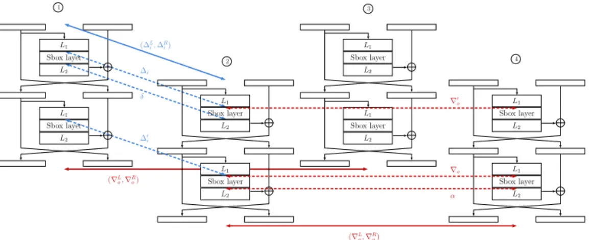
As we show next, the counterpart of this table for the Feistel case turns out to be useful to study a switch over two rounds. Following the idea of [WP19], we define it as follows (it can be visualized in Figure6):
Definition 6 (FBDT). Let S be a function from Fn
2 to itself, and (∆i, δ, ∇o) be elements of (Fn
2)3. The Feistel boomerang difference table (FBDT) of S is a three-dimensional table,
in which the entry for (∆i, δ, ∇o) is computed by:
FBDT(∆i, δ, ∇o) = #{x ∈ Fn2|S(x) ⊕ S(x ⊕ ∆i) ⊕ S(x ⊕ ∇o) ⊕ S(x ⊕ ∆i⊕ ∇o) = 0, S(x) ⊕ S(x ⊕ ∆i) = δ}. ∆i ∇o L1 R1 L2 R2 L3 R3 R4 L4 S L S S S S S L S S S S S L S S S S S L S S S S · · · · · · · · · · · · 1 2 3 4 δ x ∇o
Figure 6: View of the parameters of the FBDT: ∆i is the input difference and δ is the
output difference of S when looking at the difference between state and1 . ∇2 o is the input difference of the same Sbox S when looking at the difference between state and1
3
(which is the same as the one between state and2 ).4
Given the discussion made in Section4.7, we can rewrite the FBDT as:
FBDT(∆i, δ, ∇o) = #{(χDDT(∆i, δ)) ∩ (χDDT(∆i, δ) ⊕ ∇o)}.
This is rather straightforward to see that the FBDT follows similar relations as the BDT does, namely:
Property 3 (Relations between the DDT, FBCT and FBDT).
1. DDT (∆i, δ) = FBDT(∆i, δ, 0) = FBDT(∆i, δ, ∆i) and in the general case DDT (∆i, δ) ≥ FBDT(∆i, δ, ∇o).
2. FBCT(∆i, ∇o) =P2
n−1
δ=0 FBDT(∆i, δ, ∇o). 3. FBDT(0, 0, ∇o) = 2n.
5.2
Probability of a 2-round Boomerang Switch
The theorem we discuss next gives the probability that a boomerang comes back over 2 rounds of a classic Feistel cipher, that is a balanced one with 2 branches. We consider that the input difference between state and1 is (∆2 Li, ∆R
i ), that the output difference between state and2 and4 and1 is equal to (∇3 L
o, ∇ R
o), and we want that the input difference between state and3 is again (∆4 L
i, ∆ R i).
Again, we consider a very generic case where the round function is composed of one Sbox layer made of t parallel n-bit Sboxes and of some linear or affine operations, which implies in particular that if the input difference of one round is known together with the output difference of the Sbox layer, then the difference at the input of the next round Sbox layer can be computed. To keep our explanation as generic as possible we introduce the following notations, that can be visualized in Figure7:
• ∆i represents the difference at the input of the first round Sbox layer, between state 1
and . It is fixed to a certain value since it can be deduced from the first round2 input difference ∆L
i.
• δ denotes the corresponding output difference of this Sbox layer, but is not specified. • ∆0
i corresponds to the difference at the input of the second Sbox layer (again with respect to state and1 ). Its value is deduced from δ and from ∆2 Ri .
• In a similar way, the difference at the input of the second round Sbox layer, between state and2 is set to a certain value denoted ∇4 o, deduced from ∇Ro.
• The corresponding output difference is denoted α, but again is not fixed.
• ∇0o represents the input difference of the first round Sbox layer for these states, and
is computed from ∇L o and α. (∆L i, ∆Ri) (∇Lo,∇Ro) α 1 2 3 4 L1 Sbox layer L2 ∆i δ ∆′ i (∇Lo,∇Ro) ∇o ∇′o L1 Sbox layer L2 L1 Sbox layer L2 L1 Sbox layer L2 L1 Sbox layer L2 L1 Sbox layer L2 L1 Sbox layer L2 L1 Sbox layer L2
Figure 7: Boomerang Switch over two rounds of a balanced Feistel with two branches. The differences denoted with straight lines are imposed and fixed.
Given this notation we can find a formula for the probability of a 2-round boomerang switch over a Feistel, see Theorem 4. Note that to simplify its writing we extended the definition of the FBDT to the case of the Sbox layer (instead of one Sbox only). Naturally, this simply corresponds to the product of the FBDT of each Sbox that composes the Sbox layer.
Theorem 4 (Probability of a 2-round Switch). With the previous notation, the probability
that a boomerang comes back over 2 rounds is equal to:
2−2tn× X
0≤δ,α<2n
FBDT(∆i, δ, ∇0o) × FBDT(∇o, α, ∆0i). (3)
Proof. In order to cover most constructions, in what follows we consider a Feistel cipher
as depicted in Figure 7, that is with a round function made of one linear (or affine) layer
L1, followed by one Sbox layer of t n-bit Sboxes and again a linear (or affine) layer L2.
We start by observing that if the second round Sbox layer output difference between state and2 is equal to a given value α then the same difference is required between4 state and1 for the boomerang to return.3
Denote by α0 the second Sbox layer output difference between state and1 . Given3 that the output difference between and1 and3 and2 is equal to (∇4 L
o, ∇Ro) we deduce that the input difference in the left branch between states and1 and3 and2 4 are respectively equal to ∇Lo ⊕ L2(α0) and ∇Lo ⊕ L2(α). The input difference between the
left branches of state and1 is equal to ∆2 L
i so we deduce that the left branch difference between state and3 is equal to: ∆4 L
i ⊕∇Lo⊕L2(α0)⊕∇Lo⊕L2(α) = ∆Li ⊕L2(α0)⊕L2(α).
For the boomerang to return this has to be equal to ∆L
i, which proves that we must have
α0= α.
We now demonstrate the formula by first looking at the case where the values of α and
δ are fixed. The theorem is deduced by summing over all their possible values.
We focus on the second round of the switch, and more precisely on the difference between state and2 . To obtain the required output difference, the Sbox layer must4 transition from ∇o= L1(∇Ro) to α, an event that is of probability7:
2−nt× DDT(∇o, α).
If we denote by X the input value of the second round Sbox layer of state , We know2 that the corresponding value of state has to be equal to X ⊕ ∆1 0i, value that should also allow the transition from ∇o to α according to the previous discussion. The probability that it is the case is:
#χDDT(∇o, α) ∩ (χDDT(∇o, α) ⊕ ∆0i)
#χDDT(∇o, α)
.
Assuming that the previous conditions are fulfilled, the boomerang returns in the first round if the Sbox layer transitions from ∆i to δ given that the input difference of this Sbox layer between state and2 and4 and1 is equal to ∇3 0
o. The probability of this event is FBDT(∆i, δ, ∇0o) × 2−nt.
Putting things together, we obtain
2−2tn× X
0≤δ,α<2n
FBDT(∆i, δ, ∇0o) × DDT(∇o, α) ×
#χDDT(∇o, α) ∩ (χDDT(∇o, α) ⊕ ∆0i)
#χDDT(∇o, α)
Given that DDT(∇o, α) = #χDDT(∇o, α) and that #(χDDT(∇o, α) ∩ (χDDT(∇o, α) ⊕ ∆0i)) = FBDT(∇o, α, ∆0i), we obtain the required expression.
Note that our formula is very reminiscent of what is used in the SPN case, as Wang
and Peyrin [WP19] proposed to use the product of the BDT and BDT’ coefficients to
cover the case of a 2-round switch where the same Sbox is active with respect to E0 and
E1. As a side note, we also remark here that the somewhat more intricate formulation
proposed by Song et al. can be rewritten as the product of the BDT and BDT’ in the case of 2 rounds, as in particular the DBCT coefficient of [SQH19] is in fact equal to the BDT’ coefficient.
We show a concrete example of application of this 2-round formula on LBlock in Ap-pendixE.
6
Generic Formula for a Feistel Boomerang Switch over
Multiple Rounds
To obtain an accurate estimation of the probability of a boomerang distinguisher, an attacker has to correctly evaluate the size of Em, that is the number of middle rounds for which there exists a dependency between the characteristic on E0 and the one on E1.
Once this is done, the formula introduced with the sandwich attack theory [DKS10] can be applied and the value of p2q2r (where r is the probability of Em, p the one of E0and q
the one of E1) gives a good estimate (under the usual assumptions).
The problem of evaluating the size of Emhas already been discussed in two papers in the case of SPN ciphers: by Song et al. in [SQH19] and by Wang and Peyrin in [WP19]. The algorithm proposed in [SQH19] (that we recall in Appendix F) is rather natural: additional rounds are added to Em as long as the probability of the newly added round is higher than the probability that would have been obtained if they were no dependencies. Since this technique directly applies to boomerang distinguishers on Feistel constructions we do not elaborate more on this.
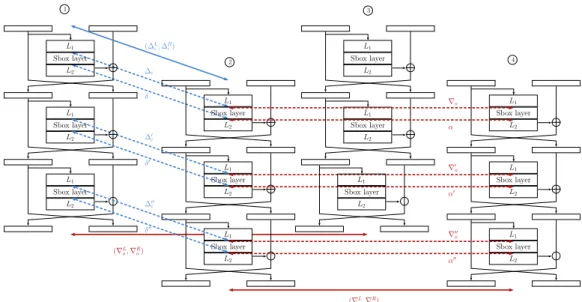
The remaining problem in the case of Feistel ciphers is to compute the probability of a boomerang switch over more than 2 rounds. We address this now, with a setting and notation given in Figure 8and that is a direct generalization of the one in Figure7.
(∆L i, ∆Ri) (∇Lo,∇Ro) α′ 1 2 3 4 L1 Sbox layer L2 ∆i δ ∆′i (∇Lo,∇Ro) ∇′ o ∇o L1 Sbox layer L2 L1 Sbox layer L2 L1 Sbox layer L2 L1 Sbox layer L2 L1 Sbox layer L2 L1 Sbox layer L2 L1 Sbox layer L2 Sbox layer L1 L2 Sbox layer L1 L2 Sbox layer L1 L2 Sbox layer L1 L2 δ′ ∆′′ i δ′′ α′′ ∇′′ o α
Figure 8: Setting for a boomerang Switch over more than two rounds of a balanced Feistel with two branches. The differences denoted with straight lines are imposed and fixed.
As depicted in the figure, we introduce new variables to represent all the intermediate differences. As we did when discussing the 2-round switch, the idea will be to iterate over all the possible values for these, to compute the probability of the obtained settings and
finally to sum together the probabilities.
We introduce a coefficient that corresponds to the situation where an active Sbox in
E0 is in front of an active Sbox in E1, and for which both Sbox outputs (when looking at
state and1 and state2 and2 ) are fixed. We obtain the following formula:4
Definition 7 (FBET). Let S be a function from Fn2, and (∆i, δ, ∇o, α) be elements of (Fn2)4.
The Feistel boomerang extended table (FBET) of S is a four-dimensional table, in which the entry for (∆i, δ, ∇o, α) is computed by:
FBET(∆i, δ, ∇o, α) = #{x ∈ Fn2|S(x) ⊕ S(x ⊕ ∆i) ⊕ S(x ⊕ ∇o) ⊕ S(x ⊕ ∆i⊕ ∇o) = 0,
S(x) ⊕ S(x ⊕ ∆i) = δ,
S(x ⊕ ∆i) ⊕ S(x ⊕ ∆i⊕ ∇o) = α}.
The probability of a switch is then estimated to be8 the sum over all the possible
intermediate differences of the product of the FBET coefficient (divided by 2n) of each Sbox. For instance, the probability of the 3-round boomerang switch depicted in Figure7can be approximated by: 2−3tn X 0≤δ,α,δ0,α0,δ00,α00<2n FBET(∆i, δ, ∇o, α) × FBET(∆0i, δ 0, ∇0 o, α 0 ) × FBET(∆00i, δ 00, ∇00 o, α 00)
where again by abuse of notation the FBET coefficient is the one of the full S-layer, but should be replaced by the ones of the individual Sboxes. Note that ∆i and ∇00o are determined by (∆Li, ∆Ri ) and (∇Lo, ∇Ro), the input and output differences of the switch. Also, the values of ∆0i, ∆00i, ∇o and ∇0oare deduced from the other parameters on which we iterate (for instance ∆0i = L1(L2(δ) ⊕ ∆Ri )).
As we show in the following property, the obtained formula can be simplified when we sum coefficients over all the possible values of some variables. Further simplifications are obtained with Property 3.
Property 4 (Relations between the FBET and the previous tables). X 0≤δ<2n FBET(∆i, δ, ∇o, α) = FBDT(∇o, α, ∆i). X 0≤α<2n FBET(∆i, δ, ∇o, α) = FBDT(∆i, δ, ∇o). FBET(0, 0, ∇o, α) = FBET(∇o, α, 0, 0) = DDT(∇o, α).
It is rather easy to show that the FBET view covers the previous formula for the 2-round switch (given in Theorem 4): we use the notation of Figure7 and additionally denote by
δ0 the output difference between state and1 of the second-round S-layer, and by α2 0 the output difference between state and2 of the first-round S-layer. The sum we have4 to compute is: 2−2tn X 0≤δ,α0,δ0,α<2n FBET(∆i, δ, ∇0o, α 0 ) × FBET(∆0i, δ 0, ∇ o, α).
8Note that this approximation considers that the same characteristic is followed between state 1 and 2
and between state 3 and 4 . For 3 rounds and more it is not apparent that this is always the only possible case.
Since α0 and δ0 have no impact on the other values we can rewrite the previous sum as: 2−2tn X 0≤δ,α0,α<2n (FBET(∆i, δ, ∇0o, α0) × X 0≤δ0<2n FBET(∆0i, δ0, ∇o, α)) = 2−2tn X 0≤δ,α0,α<2n (FBET(∆i, δ, ∇0o, α 0 ) × FBDT(∇o, α, ∆0i)) = 2−2tn X 0≤δ,α<2n (FBDT(∇o, α, ∆0i) × X 0≤α0<2n FBET(∆i, δ, ∇0o, α 0)) = 2−2tn X 0≤δ,α<2n (FBDT(∇o, α, ∆0i) × FBDT(∆i, δ, ∇0o)).
In a similar way, if we focus on one round only, we have to compute
2−tn X
0≤δ,α<2n
FBET(∆i, δ, ∇o, α).
Since both δ and α have no impact on the other variables it can be rewritten as:
2−tn X
0≤δ<2n
FBDT(∆i, δ, ∇o) = 2−tnFBCT(∆i, ∇o).
So the FBET coefficient allows to recover our previous formulas.
Note that when looking at a switch covering many rounds the application of this formula may require too much time if many Sboxes are involved, so it might be preferable to evaluate the probability of Em experimentally.
Short Discussion on the SPN Case. While we focused on the Feistel case, it seems that
a similar technique can be used to get the probability of a multiple-round boomerang switch on an SPN cipher. In particular, the counterpart of the FBET would be:
BET (∆i, δ, ∇o, α) = #{x ∈ Fn2|S−1(S(x) ⊕ ∇o) ⊕ S−1(S(x ⊕ ∆i) ⊕ ∇o) = ∆i,
S(x) ⊕ S(x ⊕ ∆i) = δ,
x ⊕ S−1(S(x) ⊕ ∇o) = α}.
and we have the following direct properties:
Property 5 (Relation between the BET and the previous tables). X 0≤α<2n BET (∆i, δ, ∇o, α) = BDT (∆i, δ, ∇o), X 0≤δ<2n BET (∆i, δ, ∇o, α) = BDT0(∇o, α, ∆i) = DBCT(∆i, ∇o, α) X 0≤α,δ<2n BET (∆i, δ, ∇o, α) = BCT (∆i, ∇o)
Our bet is that it provides a generic formula covering the previous particular cases discussed in [SQH19] and [WP19].
7
Application to LBlock-s
We propose here to study the case of LBlock-s, the Feistel cipher used in LAC, in order to illustrate the way our formula can be used to estimate the probability of a boomerang distinguisher.
LAC was a first-round candidate to the CAESAR competition submitted by Lei Zhang et al. [ZWW+14]. It is a lightweight authenticated encryption scheme that relies on a
modified version of LBlock called LBlock-s. In this version, the 10 different 4-bit Sboxes
are replaced with one unique Sbox, which corresponds to the one called S0 in LBlock.
The block cipher also includes a modified key schedule algorithm that we do not detail here since it plays no role in the following discussion. The LAC algorithm uses both full 32-round LBlock-s as well as a round-reduced LBlock-s iterating 16 rounds.
In this section, we evaluate with the p2q2r formula the probability of a 16-round
boomerang distinguisher on LBlock-s when the size of Em varies from 2 to 8 rounds.
We found out that when Em covers 8 rounds the expected probability of the resulting
distinguisher is 2−56.14.
This value is higher than the probability of the distinguisher that was proposed by Leurent in [Leu15]. In this paper, the author showed the existence of collections of differential characteristics with probability as high as 2−61.52. Still, our distinguisher cannot be used for forgery contrary to what is done in [Leu15].
7.1
Finding the Best 7-round Differential Characteristics for E
0and E
1As a starting point, we look at the setting where Emcovers 2 rounds and search the best characteristics over 7 rounds for E0 and E1. To find these, we use the two-step strategy
described in [GLMS18]:
• In the first step, we abstract all the nibble differences by Boolean variables (if a nibble is active then its associated Boolean value is 1, else it is 0) and we look for the truncated differentials with the minimum number of active Sboxes. We implement this step using a high-level modeling language called MiniZinc [NSB+07]. MiniZinc models are translated into a simple subset of MiniZinc called FlatZinc, using a compiler provided by MiniZinc. Most existing constraint programming solvers (including SAT solvers and MILP solvers) have developed FlatZinc interfaces (there are currently fifteen solvers with FlatZinc interfaces). Using the PICAT SAT solver we found 8 possible optimal truncated differential characteristics that are valid for both E0 and E1.
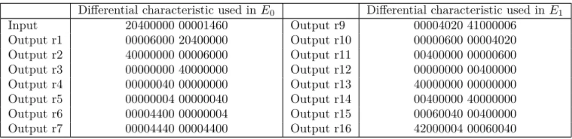
• In the second step, we look for the best differential characteristics (in terms of probability) that follow the previous truncated differential paths. To do so, we use the constraint programming language Choco [PFL16]. For each possible truncated differential characteristics on 7 rounds we obtain 2766 solutions with an optimal probability equal to 2−16. We tried several combinations and picked the one that gave the best probability for the 2-round Em. We present it in Table3.
7.2
Choosing a Switch E
mTo obtain an accurate evaluation of the boomerang distinguisher, we evaluate the size and probability of Emwith the algorithm recalled in AppendixF. When Emcovers few rounds we were able to apply our formulas to compute its probability but we then switched to experiments to avoid intricate expressions with many parameters. As detailed in Table4, we were able to apply the algorithm for an Em covering up to 8 rounds, thus obtaining an estimation of the probability of the distinguisher of 2−56.14. Our observation is that Em
Table 3: The two differential characteristics on 7 rounds of E0 and of E1in hexadecimal
notations.
Differential characteristic used in E0 Differential characteristic used in E1
Input 20400000 00001460 Output r9 00004020 41000006 Output r1 00006000 20400000 Output r10 00000600 00004020 Output r2 40000000 00006000 Output r11 00400000 00000600 Output r3 00000000 40000000 Output r12 00000000 00400000 Output r4 00000040 00000000 Output r13 40000000 00000000 Output r5 00000004 00000040 Output r14 00400000 40000000 Output r6 00004400 00000004 Output r15 00060040 00400000 Output r7 00004440 00004400 Output r16 42000004 00060040
covers more than 8 rounds, but we were limited by computational power to get its exact size.
Table 4: Theoretical and practical values of r for various sizes of Em and corresponding
probability of the 16-round distinguisher when applying the p2q2r formula. We detail the
theoretical computation for 3 rounds in Appendix G.
Em α δ theoretical r practical r p2q2r 0 rounds - - - - 2−88 2 rounds (0x00004440, 0x00004400) (0x00004020, 0x41000006) 2−3.09 2−3.09 2−67.09 3 rounds (0x00004440, 0x00004400) (0x00000600, 0x00004020) 2−6.80 2−6.80 2−62.8 4 rounds (0x00004400, 0x00000004) (0x00000600, 0x00004020) n/a 2−14.10 2−62.1 6 rounds (0x00000004, 0x00000040) (0x00400000, 0x00000600) n/a 2−19.04 2−59.04 8 rounds (0x00000040, 0x00000000) (0x00000000, 0x00400000) n/a 2−24.14 2−56.14
7.3
Deriving a Boomerang Distinguisher
The previous discussion indicates that the 16-round boomerang distinguisher we are looking at has a probability higher than 2−56.14. It can be used as follows:
The attacker randomly chooses M1
i (0 ≤ i < m) and compute Mi2 = Mi1⊕ α with α = (20400000, 00001460). She encrypts these plaintexts over 16 rounds of LBlock-s to
obtain the ciphertexts C1
i and Ci2 from which she deduces Ci3= Ci1⊕ δ and Ci4= Ci2⊕ δ
with δ = (0x42000004, 0x00060040) and asks for their corresponding plaintexts M3
i and Mi4. Finally she checks if the boomerang comes back by testing if Mi3⊕ M4
i = α.
Given our estimate, m = 256.14 quartets are sufficient to expect one boomerang to
return (using 258.14 ciphering/deciphering operations).
8
Conclusion
Starting from an observation similar to the one made by Murphy in 2011, we develop a new theory that explains the behavior of boomerang switches for Feistel ciphers. We introduce the adequate notion of FBCT and give its main properties and relations with other well-known cryptographic tables. Taking things further, we provide a rather simple expression of the probability of a boomerang switch over two rounds, and a (more intricate) general expression of the one over multiple rounds.
Acknowledgments
This work has been partly funded by the French Direction Générale des Entreprises (DGE) under grant FUI 23 PACLIDO and by the ANR under grant Decrypt ANR-18-CE39-0007.

![Figure 3: Middle rounds of the boomerang distinguisher proposed in [LGW12].](https://thumb-eu.123doks.com/thumbv2/123doknet/14248349.487837/5.892.155.734.696.991/figure-middle-rounds-boomerang-distinguisher-proposed-lgw.webp)