Challenges in Recommender Systems: Scalability,
Privacy, and Structured Recommendations
by
Yu Xin
Submitted to the Department of Electrical Engineering and Computer
Science
in partial fulfillment of the requirements for the degree of
Doctor of Philosophy in Computer Science and Engineering
at the
MASSACHUSETTS INSTITUTE OF TECHNOLOGY
June 2015
c
○ Massachusetts Institute of Technology 2015. All rights reserved.
Author . . . .
Department of Electrical Engineering and Computer Science
Mar 16, 2015
Certified by . . . .
Tommi Jaakkola
Professor
Thesis Supervisor
Accepted by . . . .
Professor Leslie A. Kolodziejski
Chairman, Department Committee on Graduate Theses
Challenges in Recommender Systems: Scalability, Privacy,
and Structured Recommendations
by
Yu Xin
Submitted to the Department of Electrical Engineering and Computer Science on Mar 16, 2015, in partial fulfillment of the
requirements for the degree of
Doctor of Philosophy in Computer Science and Engineering
Abstract
In this thesis, we tackle three challenges in recommender systems (RS): scalability, privacy and structured recommendations.
We first develop a scalable primal dual algorithm for matrix completion based on trace norm regularization. The regularization problem is solved via a constraint generation method that explicitly maintains a sparse dual and the corresponding low rank primal solution. We provide a new dual block coordinate descent algorithm for solving the dual problem with a few spectral constraints. Empirical results illustrate the effectiveness of our method in comparison to recently proposed alternatives. In addition, we extend the method to non-negative matrix factorization (NMF) and dictionary learning for sparse coding.
Privacy is another important issue in RS. Indeed, there is an inherent trade-off be-tween accuracy of recommendations and the extent to which users are willing to re-lease information about their preferences. We explore a two-tiered notion of privacy where there is a small set of public users who are willing to share their preferences openly, and a large set of private users who require privacy guarantees. We show theoretically, and demonstrate empirically, that a moderate number of public users with no access to private user information already suffices for reasonable accuracy. Moreover, we introduce a new privacy concept for gleaning relational information from private users while maintaining a first order deniability. We demonstrate gains from controlled access to private user preferences.
We further extend matrix completion to high-order tensors. We illustrate the prob-lem of recommending a set of items to users as a tensor completion probprob-lem. We develop methods for directly controlling tensor factorizations in terms of the degree of nonlinearity (the number of non-uniform modes in rank-1 components) as well as the overall number of rank-1 components.
Finally, we develop a tensor factorization for dependency parsing. Instead of manually selecting features, we use tensors to map high-dimensional sparse features into low dimensional (dense) features. Our parser achieves state of the art results across multiple languages.
Thesis Supervisor: Tommi Jaakkola Title: Professor
Acknowledgments
First and foremost, I would like to thank my advisor Prof. Tommi Jaakkola for his continuous support throughout my graduate years. He has been a great advisor and one of the smartest people I know. Whenever I encountered a problem in my research, Tommi would show me not just one, but a few different ways to solve the problem. I hope to one day gain the insight he has in this field.
I would also like to thank my committee members Alan Willsky and Leslie Kaelbling for their guidance on my thesis.
Next, I would like to thank the many smart and interesting people I met at MIT. I benefited a lot from discussions with my collaborators Tao Lei, Yuan Zhang and Yuan Luo. I also had a lot of fun with my officemates Andreea Gane, Paresh Malalur and David Reshef who made the office enjoyable. I am very grateful to Wujie Huang for his friendship over 10 years. The two of us were undergrads at Tsinghua, are currently attending MIT and will be joining the same company afterwards. I hope we will always be friends.
Finally, my biggest thanks go to my parents Xiaozhu Wang and Ziliang Xin for their infinite support, continuous encouragement and unconditional love they have always given me .
Contents
1 Introduction 15 1.1 Challenges . . . 17 1.1.1 Scalability . . . 18 1.1.2 Privacy . . . 19 1.1.3 Structured recommendations . . . 20 1.2 Summary of contributions . . . 21 2 Background 23 2.1 Matrix Factorization . . . 24 2.2 Optimization algorithms . . . 26 2.2.1 Proximal gradient . . . 27 2.2.2 Semi-definite programming . . . 28 2.3 (Differential) privacy . . . 29 2.4 Tensor factorization . . . 323.1 Derivation of the dual . . . 37
3.2 Solving the dual . . . 40
3.3 Constraints and convergence . . . 43
3.4 Non-negative matrix factorization . . . 44
3.5 Sparse matrix factorization . . . 48
3.6 Independent Component Analysis . . . 52
3.7 Experiments . . . 54
3.7.1 Primal-dual algorithm for matrix completion . . . 54
3.7.2 Non-negative matrix factorization . . . 57
3.7.3 Sparse matrix factorization . . . 60
4 Privacy mechanism 63 4.1 Problem formulation and summary of results . . . 64
4.2 Analysis . . . 68
4.2.1 Statistical Consistency of ^Σ . . . 68
4.2.2 Prediction accuracy . . . 70
4.3 Controlled privacy for private users . . . 71
4.4 Experiments . . . 75
4.5 Conclusion . . . 79
5 Tensor factorization for set evaluation 81 5.1 Notation . . . 82
5.2 Convex regularization . . . 84
5.3 Consistency guarantee . . . 89
5.4 Alternating optimization algorithm . . . 93
5.5 Experimental results . . . 96
5.6 Conclusion . . . 99
6 Extension to dependency parsing 101 6.1 Low-rank dependency parsing . . . 101
6.2 learning . . . 103
6.3 Experimental Setup . . . 105
6.4 Results . . . 108
List of Figures
1-1 Examples of Recommendation Systems . . . 17
2-1 Illustration of a statistical database . . . 29
2-2 Illustration of a statistical database . . . 31
2-3 Example of a 3-dimensional tensor . . . 32
2-4 CP decomposition (Kolda and Bader, 2009) . . . 33
3-1 test RMSE comparison of JS and PD . . . 56
3-2 Optimization progress of JS and PD . . . 56
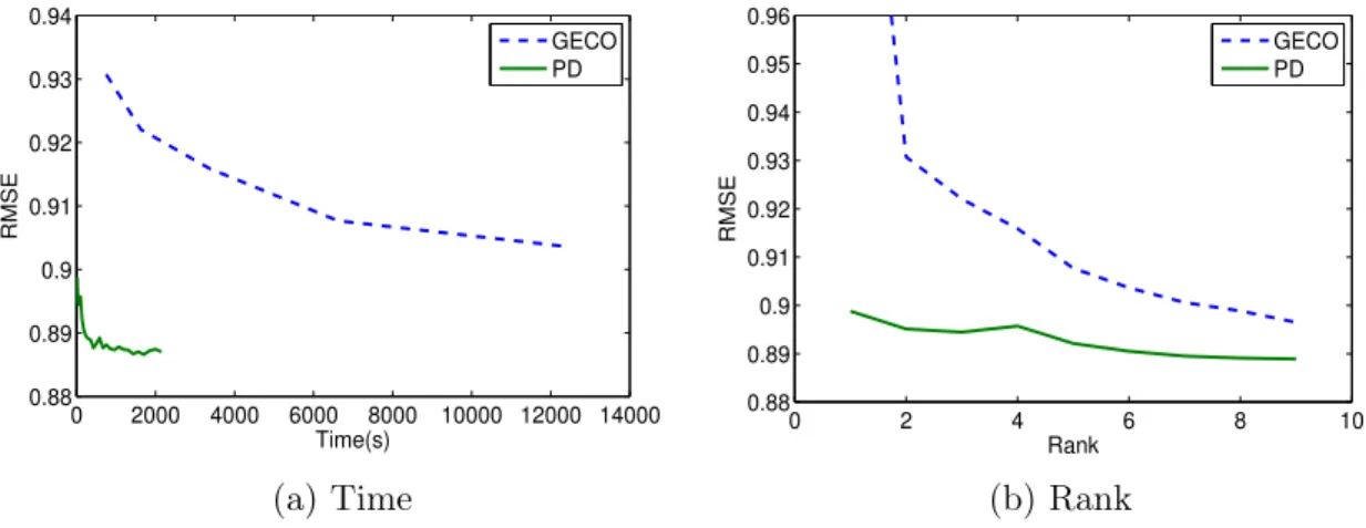
3-3 test RMSE comparison of GECO and PD . . . 57
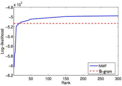
3-4 Log-likelihood comparison of NMF and Bigram for different document groups . . . 60
3-5 Left: Log-likelihood of NMF as a function of time; Right: Time as a function of rank. . . 60
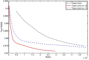
3-6 test RMSE comparison of Trace norm, Trace norm w. 𝐿0, Trace norm w. 𝐿1 regularization . . . 61
4-2 Summary of operations on both sides . . . 67 4-3 Example of ℳ(𝑟) . . . 74 4-4 Test RMSE as a function of users and ratings . . . 76 4-5 Test RMSE as a function of private user numbers. PMC: the privacy
mechanism for continuous values; PMD: the privacy mechanism for discrete values; Lap eps=1: DP with Laplace noise, 𝜖 = 1; Lap eps=5: same as before except 𝜖 = 5; SSLP eps=5: sampling strategy described in (Duchi et al., 2013) with DP parameter 𝜖 = 5; Exact 2nd order: with exact second order statistics from private users (not a valid privacy mechanism); Full EM: EM without any privacy protection. . 77
5-1 Test RMSE compared to linear regression, nonlinear regression model with second order monomials and PARAFAC tensor factorization method. The tensor completion approach with d=2 consistently performs bet-ter than the three methods with improvement (10−2): 2.66 ± 0.26, 1.77 ± 0.33 and 3.55 ± 0.86 . . . 99 5-2 Test RMSE as a function of regularization for various 𝑑 . . . 99
6-1 Average UAS on CoNLL testsets after different epochs. Our full model consistently performs better than NT-1st (its variation without tensor component) under different choices of the hyper-parameter 𝛾. . . 109
List of Tables
1.1 Example of collaborative filtering . . . 18
6.1 Word feature templates used by our model. pos, form, lemma and morph stand for the fine POS tag, word form, word lemma and the morphology feature (provided in CoNLL format file) of the current word. There is a bias term that is always active for any word. The suffixes -p and -n refer to the left and right of the current word respec-tively. For example, pos-p means the POS tag to the left of the current word in the sentence. . . 103
6.2 First-order parsing (left) and high-order parsing (right) results on CoNLL-2006 datasets and the English dataset of CoNLL-2008. For our model, the experiments are ran with rank 𝑟 = 50 and hyper-parameter 𝛾 = 0.3. To remove the tensor in our model, we ran experiments with 𝛾 = 1, corresponding to columns NT-1st and NT-3rd. The last column shows results of most accurate parsers among (Nivre et al., 2006; McDonald et al., 2006; Martins et al., 2010, 2011, 2013; Koo et al., 2010; Rush and Petrov, 2012; Zhang and McDonald, 2012; Zhang et al., 2013) . . 106
6.3 Results of adding unsupervised word vectors to the tensor. Adding this information yields consistent improvement for all languages. . . . 109
6.4 The first three columns show parsing results when models are trained without POS tags. The last column gives the upper-bound, i.e. the performance of a parser trained with 12 Core POS tags. The low-rank model outperforms NT-1st by a large margin. Adding word vector features further improves performance. . . 109 6.5 Five closest neighbors of the queried words (shown in bold). The upper
part shows our learned embeddings group words with similar syntactic behavior. The two bottom parts of the table demonstrate how the projections change depending on the syntactic context of the word. . 110 6.6 Comparison of training times across three typical datasets. The second
column is the number of tokens in each data set. The third column shows the average sentence length. Both first-order models are imple-mented in Java and run as a single process. . . 111
Chapter 1
Introduction
Personalization has become one of the key features of on-line content. For instance, Amazon frequently recommends items to customers based on their previous purchase history. Similarly, Facebook ranks and displays news feeds as to match personal inter-ests of their users. The engines behind personalization are known as recommendation systems (RS). These systems analyze the behavioral patterns of users in an attempt to infer user preferences over artifacts of interest. Figure 1-1 gives two examples of recommender systems (RS).
Most algorithms underlying RS can be seen as focusing on either content-based filter-ing (CB), collaborative filterfilter-ing (CF), or some combination of the two. CB assumes that each item to be recommended has an associated feature vector that can be used for prediction either directly or by means of evaluating similar other items. To be successful, similarity based methods require additional control of diversity to avoid overwhelming users with many items that they are already familiar with (Adomavicius and Tuzhilin, 2005).
CF in its pure form treats both users and items as symbols without assuming any additional feature representations. Nevertheless, CF methods can be used to complete the limited information about a particular user by borrowing purchase/rating histories
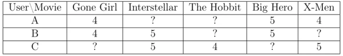
of other similar users. In this sense recommendations are based on like-minded other users rather than direct similarities between items. As a preprocessing step, user histories are first transformed into numerical values or ratings that represent users’ evaluations of items. For instance, the ratings can be the number of stars users give to movies at IMDB. They can also be binary values indicating if users select “like” or “dislike” for a Youtube video. In general, the task is to make accurate predictions of unknown ratings in the user-item table. Table 1.1 gives a simple example of movie recommendation with user provided ratings on the scale of zero to five. The question mark represents an unknown rating. In the example, users A and B have similar past ratings, giving us the means to recommend movie “Interstellar” to A by borrowing the rating from user B.
Various criteria have been proposed for evaluating RS performance. Traditional mea-sures such as mean absolute error (MAE) or root mean squared error (RMSE) are among the most commonly used, primarily due to their simplicity. Ranking measures that evaluate the order of recommended items better match the actual task since the predicted items are displayed as ordered lists (Herlocker et al., 2004; Balakrishnan and Chopra, 2012). Besides the accuracy of predicting ratings, or their rank, another important factor is diversity(Zhou et al., 2010). Methods that only highlight popu-lar, easily found items are not useful. The real value of RS comes from finding items that users would like yet be difficult to find otherwise. While important, we will not consider diversity in this thesis.
The main statistical difficulty in RS comes from the fact that observations are sparse in the sense that each user has rated only a small portion of the items. In the extreme case, a newly joined user has no previous ratings. To provide useful predictions even for new users, Melville et al. (2002) propose a hybrid method of CF and CB where items have additional attributes (beyond their ids) that can be relied upon. Ma et al. (2011) use data from social network to impose additional regularization on CF. Our focus in this thesis on CF alone, without access to additional features.
Most basic CF algorithms assume that users’ interests are static and therefore increas-ingly recoverably with additional observation. Of course, in practice, user interests change with time(Koychev and Schwab, 2000). Classical time-window approaches do not work well to offset this problem since the data are already sparse. Koren (2010) propose a method that separates transient effects from long term patterns, i.e., ex-plicitly modeling time dependent behavior of users. As we focus on the optimization and theoretical results, we will adopt the static user assumption in this thesis.
Figure 1-1: Examples of Recommendation Systems
1.1
Challenges
While RS have been widely adopted and studied for over a decade, a few key challenges remain. The focus of this thesis is on three of these challenges: scalability, privacy,
User\Movie Gone Girl Interstellar The Hobbit Big Hero X-Men
A 4 ? ? 5 4
B 4 5 ? 5 ?
C ? 5 4 ? 5
Table 1.1: Example of collaborative filtering
and structured recommendations.
1.1.1
Scalability
The amount of data used as input to RS is growing quickly as more users and items are added. For a popular website, for example, the size of stored user behavior data can easily reach TBs per day. Despite the large amount of data, most RS aspire to respond interactively in less than a second in order to keep users engaged. A key challenge here is to design efficient learning algorithms that can handle such large scale datasets.
CF algorithms cannot operate on users independently. Instead, the algorithms have to learn jointly from the experience of all users; this is time consuming with large numbers of users. For example, 𝑘 − 𝑁 𝑁 method (Resnick et al., 1994) first finds a neighborhood for each user by thresholding similarity scores or finding k most similar users. It then generates predictions by calculating weighted average of the neighboring users’ ratings. Because similarities among all pairs of users are computed, the running time of the method is quadratic in the number of users.
Several approaches have been proposed to deal with the scalability issue. Das et al. (2007) use an online learning algorithm that processes each user and updates param-eters sequentially. The online learning algorithm is generally more efficient than the batch method as it incorporates updates immediately instead of waiting to process the cumulative batch of data from all users at once . Gemulla et al. (2011) propose a distributed algorithm in which most of the computations could be conducted on multiple machines in parallel.
Most RS can be modeled as a matrix completion problem with rows being users, columns being items and entries being ratings (Koren et al., 2009; Srebro et al., 2003). The goal is to complete the matrix given partially observed entries. In this thesis, we focus on a particular method for matrix completion that uses trace norm regularization (Jaggi and Sulovsk, 2010; Xin and Jaakkola, 2012; Yang and Yuan, 2013; Ji and Ye, 2009). The model is desired because the optimization problem associated with it is convex. The convexity guarantees that any local minimum is also a global minimum, and therefore the final result does not depend on the initialization and its convergence property can be theoretically analyzed. However, the associated convexity creates a difficulty in optimization. Many proposed algorithms only work for small data sets. We propose a new primal dual algorithm that improves the efficiency for large data sets significantly.
1.1.2
Privacy
With an understanding of the value of user data, most websites are collecting as much user data as possible. This approach raises privacy concerns because the data may contain sensitive information that the users wish to keep private, e.g. users’ addresses and payment history. Although occasionally users are presented with privacy policies concerning the usage of data, they usually have no explicit control over the data. Most research on privacy protection focuses on the task of publishing data from a central database such as medical records collected by hospitals. The privacy mech-anisms can be separated into two types: interactive and non-interactive. In the non-interactive setting, a “sanitized” version of the data are published. All following operations will be conducted on the sanitized version. Methods in this setting involve data permutation and removing identifier information such as names and addresses (Sweeney, 2002; Machanavajjhala et al., 2007). However, without specified utilities of the data, general sanitization methods may not obtain satisfying results (Chawla et al., 2005). In addition, the sanitized data could still be used to identify users when
side information is provided. For example, Netflix released user rating data for their recommendation competition by removing all identifiers. Barbaro et al. (2006) show that the Netflix users can still be identified by referencing public IMDB user data due to the fact that it is rare for two different users to share a very similar taste in movies.
In contrast, interactive setting allows users to pose queries about the data and receive (possibly noisy) data. A commonly used concept in this setting is Differential Privacy (DP). DP guarantees that in the query response, it is difficult to determine if a user is in the database or not. Unlike the anonymity approach, privacy is guaranteed even if an adversarial user has additional background information. The most popular method of implementing DP is by adding noise to the query response. The level of noise depends on the sensitivity of the query function to a single data record. For statistical queries such as finding the mean or maximum, it has been proven that simply adding Laplace noise will suffice.
Despite the nice theoretical results, setting up a secure central database for RS that holds all user data is difficult. In particular, it requires users to release their own data to a trusted system that operates in a restricted manner. Considering the potential business interests that are involved and the complexity of restrictions applied to the system, the setting can be unrealistic. In this thesis, we consider a distributed setting. Each user protects his data in a personal computer. They only share limited information to a central server. Thus privacy can be preserved. We will specify the privacy notation and mechanisms in chapter 4.
1.1.3
Structured recommendations
Current RS predict individual items that users may want. An interesting extension is to predict preferences for sets of items. For instance, if the system figures out that a user is going skiing for the first time, it can recommend a pair of boots, goggles, helmet and ski pants that have matching colors and price levels. In this way, a user
can obtain everything that he or she needs for skiing with a single purchase.
There are two challenges in structured recommendations. First, the number of pos-sible sets grows exponentially with the group size. Considering that the number of items is already very large, the efficiency of learning algorithms could be an issue. Second, unlike individual items, it is unclear how to select the right score function for sets. For instance, a simple approach for approximating the scoring of a set is to find the average of the score of items in the set. Then the problem reduces to learning a score for each individual item and thus can be solved efficiently. However, this approach is weak because it ignores interactions between items.
To incorporate higher order interactions in score function for sets, one can use a tensor regularization framework. Tensors are generalizations of vectors and can be represented as multi-dimensional arrays. By definition, a first order tensor is a vector, a second order tensor is a matrix, and so on. Each axis in a tensor is called a mode. Common matrix concepts such as rank and maximum eigenvalue are also defined for tensors. Tensors are more powerful than matrices because they permit one to model high order interactions among its modes. However unlike matrices, computing these values are usually NP-hard (Hillar and heng Lim, 2009). In chapter 5, we propose a new convex regularizer for tensor that allows us to explicitly control the order of interactions among items in sets.
1.2
Summary of contributions
We summarize here the main contributions of this thesis addressing many of the key challenges raised in the previous section.
1. We propose an efficient primal dual algorithm for CF with trace norm regularization.
explicitly maintains a sparse dual and the corresponding low rank primal solution. We provide a new block coordinate descent algorithm for solving the dual problem with few spectral constraints. Empirical results illustrate the effectiveness of our method in comparison to recently proposed alternatives. We also extend the method to non-negative matrix factorization, sparse coding and independent component analysis. 2. We develop a new privacy mechanism for RS
We explore a two-tiered notion of privacy where there is a small set of “public” users who are willing to share their preferences openly, and a large set of “private” users who require guaranteed privacy. We show theoretically and demonstrate empirically that a moderate number of public users with no access to private user information suffices for reasonable accuracy. Moreover, we introduce a new privacy concept for gleaning additional information from private users while maintaining a first order deniability. We demonstrate gains from controlled access to private user data.
3. We build a tensor model for set recommendations
We formulate the scores of sets via tensors. With a new convex regularizer of tensors, we can explicitly control the order of interactions modeled in the score function. We develop an efficient algorithm for estimating the tensor efficiently that iteratively adds low rank-1 tensors. We analyze statistical consistency of the estimation problem and apply the method to set recommendations.
We apply tensors to dependency parsing. By constraining tensors to have low rank, we obtain low dimensional embeddings that are tailored to the syntactic context of words. Our parser consistently outperforms the Turbo and MST parsers across 14 languages. We also obtain the best published unlabeled attachment scores (UAS) results on 5 languages.
Chapter 2
Background
Observations in RS consist of user ID, item ID and rating value. The rating value indicates the user’s preference about the item. The observation data can be repre-sented in a matrix format with rows being users, columns being items, entries being the corresponding rating values. As was discussed in the previous section, each user has only a few ratings, so the matrix is sparsely filled. For instance, in Netflix rec-ommendation challenge dataset, the averaged user rated around 200 movies within 17770 total movies. Mathematically, the goal is to predict and fill in the missing entries based on the observed entries. The recommended items are those with the highest predicted ratings.
In general, prediction accuracy relates to the number of observed ratings. Since in many RS the ratio of observed ratings can be well below 1%, strong regularization is required during estimation. In the following, we discuss in detail most commonly used assumptions and regularizations for RS.
2.1
Matrix Factorization
Consider RS with 𝑛 users and 𝑚 items. The underlying complete rating matrix to be recovered is ˚𝑋 ∈ R𝑛×𝑚. We assume that entries are observed with noise. Specifically,
𝑌𝑖,𝑗 = ˚𝑋𝑖,𝑗+ 𝜖𝑖,𝑗, (𝑖, 𝑗) ∈ Ω (2.1)
where Ω is the set of observed ratings and noise is 𝑖.𝑖.𝑑 and follows a zero-mean sub-Gaussian distribution with parameter ‖𝜖‖𝜓2 = 𝜎. We refer to the noise distribution as
𝑆𝑢𝑏(𝜎2) (see (Vershynin, 2010)). For each observed rating, we have a loss term that is a penalty based on the difference of the observed rating to the predicted rating. To predict missing ratings, additional assumptions are required.
A typical assumption in RS is that only a few underlying factors affect users’ prefer-ences. Mathematically, the assumption suggests that matrix ˚𝑋 can be divided into a product of two smaller dimensional matrices, 𝑈 𝑉𝑇, where 𝑈 ∈ R𝑛×𝑑 and 𝑉 ∈ R𝑚×𝑑 with 𝑑 ≪ 𝑚, 𝑛 (Fazel et al., 2001; Srebro et al., 2005). 𝑈 is the user factor matrix and 𝑈𝑖 is a 𝑑-dimensional feature column vector for user 𝑖. Correspondingly, 𝑉𝑗 is the
𝑑-dimensional feature vector for item 𝑗. Their inner product 𝑈𝑖𝑉𝑗𝑇 is then user 𝑖’s
rating value for item 𝑗.
It is usually beneficial to add additional regularizations to 𝑈 and 𝑉 in order to avoid over-fitting. The optimization problem is then given by,
min 𝑈 ∈R𝑛×𝑑,𝑉 ∈R𝑚×𝑑 ∑︁ (𝑖,𝑗)∈Ω Loss(𝑌𝑖,𝑗, 𝑈𝑖𝑉𝑗𝑇) + 𝜆‖𝑈 ‖ 2 𝐹 + 𝜆‖𝑉 ‖ 2 𝐹 (2.2)
The loss function is typically convex and becomes zero when 𝑌𝑖,𝑗 = 𝑈𝑖𝑉𝑗𝑇. The most
popular choice is the squared loss, which corresponds to assuming that the noise is Gaussian (Srebro et al., 2003). Other loss functions such as hinge loss and absolute error have also been used (Srebro et al., 2005).
referred to as the low rank assumption. The factorization assumption has a few clear advantages. First, 𝑈 and 𝑉 are more efficient representation than the full matrix ˚𝑋. Second, the associated optimization problem is easier due to a smaller quantity of variables. Finally, computation of the prediction 𝑈𝑇
𝑖 𝑉𝑗 is efficient which only takes
𝑂(𝑑) operations.
The optimization problem in (2.2) can be solved approximately by an alternating minimization algorithm. In each iteration, 𝑉 is fixed and minimizing 𝑈𝑖 reduces
to a simple linear regression. Then 𝑈 is fixed and 𝑉 is minimized. The algorithm continues until 𝑈 and 𝑉 converge. It can be shown that the objective decreases in each iteration and that the algorithm is guaranteed to converge. However, the objective is not convex in 𝑈 and 𝑉 jointly. Consequently, the algorithm is only guaranteed to find a local optimum while finding a global optimum is hard (Srebro et al., 2003). The resulting local optimum depends on the initialization. As initialization is typically random, the results vary. Additionally, it is also difficult to theoretically analyze the performance of the algorithm. Non-convexity arises from the low rank constraint. Its convex relaxation is a trace norm (a.k.a nuclear norm) that is a 1-norm penalty on the singular values of the matrix (Srebro et al., 2004b)
‖𝑋‖* =
∑︁
𝑖
𝑠𝑖(𝑋) (2.3)
where 𝑠𝑖(𝑥) is the 𝑖𝑡ℎ singular value of 𝑋. With sufficient regularization, trace norm
leads to a low rank solution. A trace norm is also associated with the factorizations since it can be shown that
2‖𝑋‖* = min 𝑈,𝑉 ‖𝑈 ‖ 2 𝐹 + ‖𝑉 ‖ 2 𝐹, s.t. 𝑈 𝑉 𝑇 = 𝑋 (2.4)
Notice that the minimization does not constrain the dimensionality of 𝑈 and 𝑉 , therefore the regularization term in (2.2) is an upper bound on ‖𝑋‖*. Replacing the
regularization term of 𝑈 and 𝑉 with a trace norm, we get min 𝑋∈R𝑛×𝑚 ∑︁ (𝑖,𝑗)∈Ω Loss(𝑌𝑖,𝑗, 𝑋𝑖,𝑗) + 𝜆‖𝑋‖* (2.5)
The optimization is now convex, thus all local optima are also global optima.
2.2
Optimization algorithms
One key difficulty with the trace norm regularization approach is that while the resulting optimization problem is convex, it is not differentiable. A number of ap-proaches have been suggested to deal with this problem (e.g. Beck and Teboulle, 2009). In particular, many variants of proximal gradient methods (e.g. Ji and Ye, 2009) are effective as they are able to fold the non-smooth regularization penalty into a simple proximal update that makes use of a singular value decomposition. An alternative strategy would be to cast the trace-norm itself as a minimization problem over weighted Frobenius norms that are both convex and smooth.
Another key difficulty arises from the sheer size of the full rating matrix, even if the observations are sparse. This is a problem with all convex optimization approaches (e.g., proximal gradient methods) that explicitly maintain the predicted rating matrix (rank constraint would destroy convexity). The scaling problem can be remedied by switching to the dual regularization problem in which dual variables are associated with the few observed entries (Srebro et al., 2005). The standard dual approach would, however, require us to solve an additional reconstruction problem (using complemen-tary slackness) to realize the actual rating matrix. Next, we discuss two algorithms that are particularly designed for this optimization problem.
2.2.1
Proximal gradient
Non-smooth objectives frequently occur in sparse regularization problems such as Lasso and group Lasso (Tibshirani, 1996; Meier et al., 2008). A general method that uses proximal gradient (Parikh and Boyd, 2013), a substitute of gradient, has shown promising results across a variety of problems. The method assumes the objective can be split into two components:
min
𝑥 𝑔(𝑥) + ℎ(𝑥) (2.6)
where 𝑔(𝑥) is convex and differentiable, and ℎ(𝑥) is convex and possibly non-differentiable. The proximal mapping of ℎ(𝑥) is
proxℎ(𝑥) = argmin𝑢 (︂ ℎ(𝑢) + 1 2‖𝑢 − 𝑥‖ 2 2 )︂ (2.7)
Then the proximal gradient algorithm updates 𝑥𝑘 in the 𝑘-th iteration as
𝑥𝑘= prox𝑡 𝑘ℎ(︀𝑥 𝑘−1− 𝑡 𝑘∇𝑔(𝑥𝑘−1) )︀ (2.8)
where 𝑡𝑘 > 0 is the step size determined by line search. It is easier to interpret the
algorithm by expanding the proximal operator,
𝑥𝑘 = argmin𝑢 (︂ ℎ(𝑢) + 𝑔(𝑥𝑘−1) + ∇𝑔(𝑥𝑘−1)𝑇(𝑢 − 𝑥𝑘−1) + 1 2𝑡‖𝑢 − 𝑥 𝑘−1‖2 2 )︂ (2.9)
Indeed the algorithm finds 𝑥𝑘, and minimizes a quadratic approximation to the
orig-inal objective around 𝑥𝑘−1. The analysis of proximal gradient method is similar to that of the traditional gradient method. With appropriate step size 𝑡𝑘, the algorithm
is guaranteed to coverge to the global optimum. A typical choice for 𝑡𝑘is the Lipschitz
constant of the gradient of 𝑔(𝑥) (Parikh and Boyd, 2013).
The proximal gradient method requires that the proximal mapping can be computed efficiently. Let 𝑋 ∈ R𝑛×𝑛 be a matrix with singular vector decomposition (SVD)
𝑋 = 𝑃 𝑆𝑄𝑇 with 𝑆 = diag(𝑠
1, ..., 𝑠𝑛 ), 𝑃 and 𝑄 being unitary, we have
prox𝑡‖𝑋‖*(𝑋) = 𝑃 diag(𝜂𝑡(𝑠1), . . . , 𝜂𝑡(𝑠𝑛))𝑄𝑇 (2.10)
where 𝜂𝑡(𝑠) = max(𝑠 − 𝑡, 0) is the soft-thresholding operator (Toh and Yun, 2010).
The operator removes all the singular values that are less than 𝑡, thus generating a low rank solution. Despite the simplicity of the algorithm, the key step in SVD takes 𝑂(𝑛3) computations. Although a few improvements have been proposed that consider the intermediate solution 𝑋𝑘 has low rank, the algorithm remains slow for large 𝑛.
2.2.2
Semi-definite programming
Another method is to transform the original problem (2.5) into a semi-definite pro-gram (SDP) (Jaggi et al., 2010). Assuming 𝑋 = 𝑈 𝑉𝑇, by introducing 𝑍 =
⎛ ⎝ 𝑈 𝑉 ⎞ ⎠ (︁ 𝑈𝑇 𝑉𝑇 )︁ such that tr(𝑍) = ‖𝑈 ‖2 𝐹 + ‖𝑉 ‖2𝐹, a constrained version of (2.5) is min 𝑍∈S(𝑛+𝑚)×(𝑛+𝑚), 𝑍⪰0, tr(𝑍)=𝑡 ∑︁ (𝑖,𝑗)∈Ω Loss(𝑌𝑖,𝑗, 𝑍𝑖,𝑗+𝑛) (2.11)
Where S is the set of symmetric matrices and 𝑍 ⪰ 0 means 𝑍 is positive semi-definite. The advantage of this transformation is that many SDP algorithms can be applied (Srebro et al., 2004b). In particular, the algorithm proposed in (Hazan, 2008) is suitable for the trace constraint. In each iteration, the gradient of the objective 𝐺(𝑍) is computed. 𝐺(𝑍) is a symmetric matrix of the same size as 𝑍 with dominant eigenvector 𝑣. Instead of updating 𝑍 along 𝐺(𝑍), the algorithm updates along 𝑣𝑣𝑇,
𝑍𝑘 = 𝑍𝑘−1+ 𝛼(𝑡𝑣𝑣𝑇 − 𝑍𝑘−1) (2.12)
where 𝛼 is the step size that can be fixed or optimized. It is easy to show that the update satisfies the trace constraint tr(𝑍𝑘) = 𝑡.
Compared to the proximal gradient approach, the major step is finding the maximum eigenvector 𝑣, which can be solved efficiently by the power method. Therefore the algorithm is suitable for large scale RS. However, the algorithm is designed for SDP and not specifically tailored to trace norm regularization. In the next chapter, we will describe a novel primal dual algorithm that shows significant improvements, both theoretically and empirically.
2.3
(Differential) privacy
Besides scalability, privacy in RS has recently become a key research question. The concepts originate from the need to ensure guarantees when releasing data for a centralized database, such that no original records can be revealed. One of the most popular frameworks in the privacy literature is Differential Privacy (DP) (Dwork et al., 2006; Dwork, 2006; Alvim et al., 2012; Duchi et al., 2012).
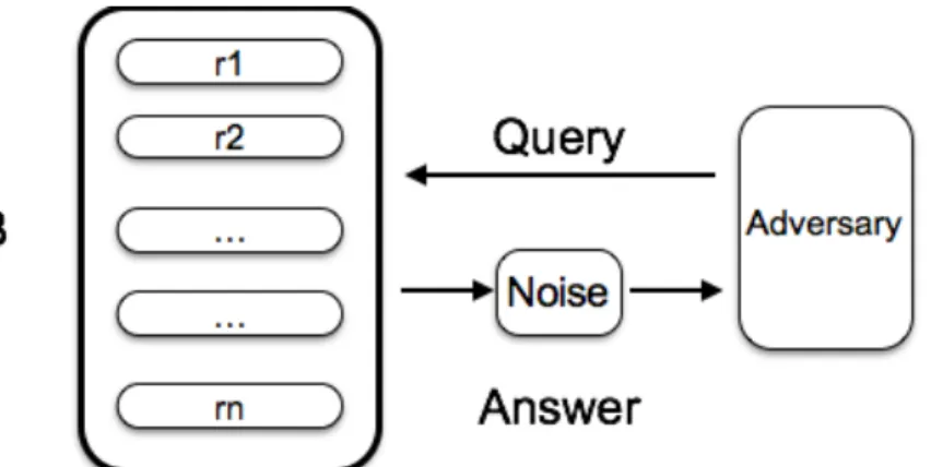
DP assumes a database that users send statistical queries to and receive answers from as illustrated in figure 2-1. The queries can be, for example, finding the maximum or mean of a particular column in the database. Assuming some of the users are adversarial, the privacy goal in this setting is to prevent adversaries from inferring any of the original records based on answers they receive.
A precise answer to a query could potentially reveal original records. For instance, assuming there are only two records in the DB, and user already knows one but not the other. By asking the mean of the two records, the user can easily infer the value of the other record. To protect privacy, the answers have to be masked with noise in this setting.
One guarantee that has been proposed to achieve privacy is 𝑘-anonymity (Sweeney, 2002). Assuming each record in the database contains information about a different person, 𝑘-anonymity requires that a person cannot be distinguished from another 𝑘 − 1 individuals in the database. The indistinguishableness gives deniability to each persona thus protecting privacy to a certain extent. However, the approach does not work for a high dimensional database because an unacceptably high amount of information would be lost (Aggarwal, 2005).
DP offers the privacy guarantee that it is difficult to differentiate if a record is con-tained in the database or not . Mathematically, let 𝐴 be the answer to a query, 𝑟𝑖 be
the 𝑖-th record, then
exp−𝜖 ≤ Pr(𝐴 = 𝛼|𝑟𝑖 ∈ DB)
Pr(𝐴 = 𝛼|𝑟𝑖 ∈ DB)/
≤ exp𝜖, ∀𝑖, ∀𝛼 (2.13)
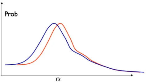
where 𝜖 is a small constant that controls the degree of privacy preservation. The difference of the two conditional distributions in (2.13) is illustrated in Figure 2-2. The blue and red lines indicate the distributions of query answers of two databases that differ by one record. Notice that the constraint is required to hold for all records and all 𝛼.
It turns out that for most queries, DP can be achieved by simply adding Laplace noise to the exact answers (Dwork et al., 2006). Let ˚𝛼 and ˚𝛼−𝑖 be the exact answers
with and without record i, and let 𝑏 be the sensitivity of the query function defined as the maximum absolute change of the function by varying one record in the database.
Figure 2-2: Illustration of a statistical database
Then the noisy answer is
𝐴 = ˚𝛼 + 𝜖, 𝜖 ∼ Lap(0,𝑏
𝜖) (2.14)
To see the the noisy answer satisfies DP, Pr(𝐴 = 𝛼|𝑟𝑖 ∈ DB)
Pr(𝐴 = 𝛼|𝑟𝑖 ∈ DB)/
= Pr(𝜖 = 𝛼 − ˚𝛼) Pr(𝜖 = 𝛼 − ˚𝛼−𝑖))
≤ exp𝜖|˚𝛼−˚𝑏𝛼−𝑖| ≤ exp𝜖 (2.15)
The other direction can be proved similarly. The result can be easily extended to multiple queries by computing the posterior distribution. For 𝑘 queries, the DP parameter is 𝑘𝜖. Therefore, the more amount of queries an adversary can make, the larger amount of noise has to be added.
DP is a very strict requirement. The amount of noise it requires may be so large such that the answer does not contain any useful information, especially if the database is small. In chapter 4, we introduce another privacy mechanism whose guarantees better fits RS.
2.4
Tensor factorization
In RS, access to side information such as time, user demographics or item descrip-tion often improves predicdescrip-tion accuracy. For instance, season is usually important for recommending clothes. One way to use side information is to build a comple-mentary model solely based on the side information, then combine this model with collaborative filtering. However, interactions of side information with user or item are ignored.
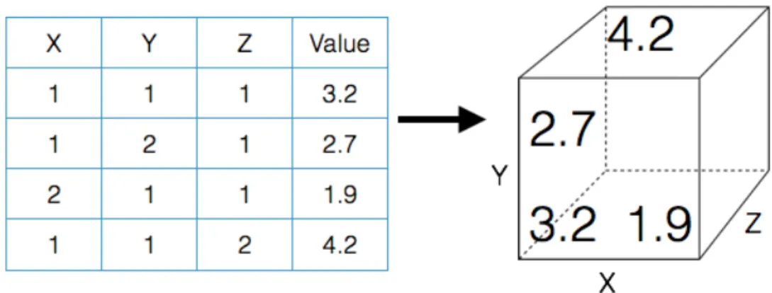
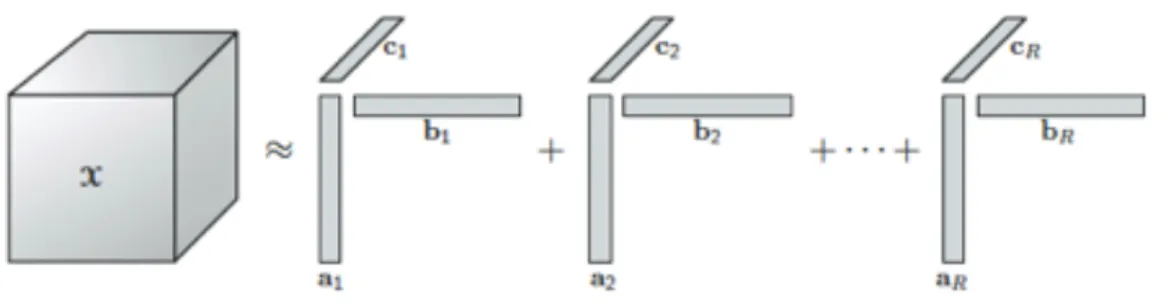
Another approach is to treat side information equally along with user and item ids. In the example of recommending clothes, the data are tuples [𝑢𝑠𝑒𝑟, 𝑖𝑡𝑒𝑚, 𝑠𝑒𝑎𝑠𝑜𝑛, 𝑟𝑎𝑡𝑖𝑛𝑔]. We can arrange such data into a multi-dimensional array, also called a tensor. Figure 2-3 shows an example of a 3-dimensional tensor. Each dimension is referred to as a mode.
Figure 2-3: Example of a 3-dimensional tensor
One way to construct a tensor is using the Kronecker product, denoted as ⊗, that is an extension of the outer product. For example, a rank one matrix 𝑇 = 𝑎𝑏𝑇 can
also be represented as 𝑇 = 𝑎 ⊗ 𝑏. Similarly, a tensor that is composed of a Kronecker product of only vectors has rank one. Any tensor 𝑇 can be decomposed into a sum of rank-1 tensors. Assume 𝑇 has 3-modes, then
𝑇 =∑︁
𝑖
To represent a tensor efficiently, we may approximate it as a sum of at most R rank-1 tensors as illustrated in Figure 2-4. If we use 𝐿2 error to measure the approximation
error, the approach is called CP-decomposition and is considered an extension of SVD for a matrix (Kolda and Bader, 2009).
Figure 2-4: CP decomposition (Kolda and Bader, 2009)
Low rank constraint is commonly used as a regularization in optimization problems (Karatzoglou et al., 2010; Rendle and Schmidt-Thieme, 2010b). Although the ob-jective with an explicit rank constraint is non-convex, a local optimum is easy to find. In Chapter 5, we introduce a new regularizer that is a convex relaxation to the rank constraint. We then apply the regularizer to set recommendation problems. In Chapter 6, we use low rank tensor for dependency parsing and obtain the state of the arts results.
Chapter 3
Primal dual algorithm
Matrix completion aims to make predictions on the missing entries of a rating matrix based on its sparsely observed entries. Since only limited information is available about each user, strong regularity assumptions are needed about the underlying rat-ing matrix. For example, we may assume that the ratrat-ing matrix has low rank, or introduce a trace norm as a convex regularizer (1-norm over the singular values of the matrix)Fazel et al. (2001); Srebro et al. (2004a). A number of algorithms have been developed for solving such, convex, regularization problems (e.g., Srebro et al. (2004a); Ji and Ye (2009); Jaggi and Sulovsk (2010); Xin and Jaakkola (2012)). The assertion of low rank assumption has been applied beyond regular matrix comple-tion. One such example is Non-negative Matrix Factorization (NMF) which intends to factorize a matrix into a product of two low dimensional non-negative matrices (Lee and Seung, 1999, 2001). It comes from the observation that most data is inherently non-negative and some data also requires additive property of different components. NMF is widely used in face recognition (Lee and Seung, 1999; Hoyer, 2004), doc-ument clustering (Xu et al., 2003; Shabnaz et al., 2006), and gene expression data analysis (Gao and Church, 2005; Kim and Park, 2007). Ding et al. (2008) have shown that NMF is closely related to Probabilistic Latent Semantic Indexing (PLSI) with a particular loss function.
The objective function of NMF is non-convex and therefore local optima exist. The optimization problem can be solved by an alternating minimization algorithm that iteratively optimizes each factor, followed by projecting to non-negative space (Kim and Park, 2007). Lee and Seung (2001) propose a different method that involves multiplicative updates that decreases the objective function while preserving non-negativity at the same time. In general, because of non-convexity of the objective function, solving NMF exactly is NP-hard (Vavasis, 2009). A side effect of NMF is that its resulting factors are usually sparse. This is because during optimization, many variables reach the boundary of constraints are automatically set to zeros. Hoyer (2004) shows that by adding an additional minimum limit on entry values, we can explicitly control the sparsity of resulting factors for easy interpretation.
Another variety of matrix factorization is dictionary learning for sparse coding which imposes a sparsity regularization constraint on one of the factors (Lee et al., 2007; Mairal et al., 2010a). Recently, it has been applied to image de-noising (Mairal et al., 2008), image classification (Mairal et al., 2009; Yang et al., 2009) and audio processing (Zibulevsky and Pearlmutter, 2001). The dictionary serves as a set of bases for reconstruction, and the corresponding coding is sparse such that only a few bases are active. The model was originally used to understand neural coding from sensor signals (Olshausen and Field, 1996) . It enjoys a few desirable properties including providing high dimensional and nonlinear representations and allowing over-complete bases.
The major optimization difficulty of sparse coding comes from 𝐿1 regularization. A
number of efficient algorithms have been suggested to solve the problem. Lee et al. (2007) propose an alternating optimization approach that updates the coding by first identifying an active set of features and then optimizing only on that set. The running time of each iteration is linear to the number of instances, therefore could be slow for large scale problems. Mairal et al. (2010a) suggested an online learning algorithm that updates the dictionary by processing instances in sequence. Their empirical results show a significant running time decrease.
We introduce here a new primal-dual approach for matrix completion that scales well to large and especially sparse matrices. Empirical results illustrate the effectiveness of our method in comparison to recently proposed alternatives. We then extend the approach to NMF and dictionary learning for sparse coding. Both of the two problems suffer non-convex objective functions. Following the trace norm, we introduce new norms of matrices that implicitly induce non-negativity, sparsity or both. By com-bining the norms with loss functions, we derive the new optimization problems that are convex relaxations to the original. The primal-dual approach can be applied to solve these problems with slightly different subproblems of finding the most violated constraints.
3.1
Derivation of the dual
It can be shown that the trace norm of matrix 𝑋 with factorization 𝑋 = 𝑈 𝑉𝑇 is equivalent to (e.g. Srebro et al., 2005)
‖𝑋‖* = min 𝑈 𝑉𝑇=𝑋 1 2(‖𝑈 ‖ 2 𝐹 + ‖𝑉 ‖ 2 𝐹) (3.1)
where 𝑈 and 𝑉 need not be low rank so that the factorization always exists. Consider then an extended symmetric matrix
𝑊 = ⎛ ⎝ 𝑈 𝑈𝑇 𝑈 𝑉𝑇 𝑉 𝑈𝑇 𝑉 𝑉𝑇 ⎞ ⎠ (3.2)
whose upper right and lower left components equal 𝑋 and 𝑋𝑇, respectively. As a result, ‖𝑋‖* = min𝑊𝑈 𝑅=𝑋tr(𝑊 )/2 where 𝑊𝑈 𝑅 is the upper right part of 𝑊 . By
We can also expand the observations into a symmetric matrix 𝑍 = ⎛ ⎝ 0 𝑌 𝑌𝑇 0 ⎞ ⎠ (3.3)
and use Ω as the index set to identify observed entries in the upper right and lower left components of 𝑍. Formally, Ω = {(𝑖, 𝑗)|1 ≤ 𝑖, 𝑗 ≤ 𝑚+𝑛, (𝑖, 𝑗−𝑛) 𝑜𝑟 (𝑖−𝑛, 𝑗) ∈ 𝐷}. With these definitions, the primal trace norm regularization problem is equivalent to the extended problem
min
𝑊 ∈𝑆
∑︁
(𝑖,𝑗)∈Ω
Loss(𝑍𝑖,𝑗− 𝑊𝑖,𝑗) + 𝜆tr(𝑊 ) (3.4)
where 𝑆 is the cone of positive semi-definite matrices in R(𝑚+𝑛)×(𝑚+𝑛).
We introduce dual variables for each observed entry in 𝑍 via Legendre conjugate transformations of the loss functions.
Loss(𝑧) = max
𝑞 {𝑞𝑧 − Loss *
(𝑞)} (3.5)
The Lagrangian involving both primal and dual variables is then given by
ℒ(𝐴, 𝑋, 𝑍) = ∑︁ (𝑖,𝑗)∈Ω [︂ 𝐴𝑖,𝑗(𝑍𝑖,𝑗− 𝑋𝑖,𝑗) − Loss*(𝐴𝑖,𝑗) ]︂ + 𝜆𝑡𝑟(𝑋) (3.6)
where 𝐴 can be written as
𝐴 = ⎛ ⎝ 0 𝑄 𝑄𝑇 0 ⎞ ⎠ (3.7)
and 𝑄 is sparse such that 𝑄𝑖,𝑗 = 0 is (𝑖, 𝑗) /∈ 𝐷. To introduce the dual variables for
as
𝑆* = {𝐸 ∈ R(𝑚+𝑛)×(𝑚+𝑛), tr(𝐸𝑇𝑀 ) ≥ 0, ∀𝑀 ∈ 𝑆} (3.8)
𝑆 is self-dual so that 𝑆* = 𝑆. The Lagrangian is then
ℒ(𝐴, 𝐸, 𝑋, 𝑍) = ∑︁ (𝑖,𝑗)∈Ω [︂ 𝐴𝑖,𝑗(𝑍𝑖,𝑗− 𝑋𝑖,𝑗) − Loss*(𝐴𝑖,𝑗) ]︂ +𝜆𝑡𝑟(𝑋) − tr(𝐸𝑇𝑋) (3.9)
To solve for 𝑋, we set 𝑑/𝑋 ℒ(𝐴, 𝐸, 𝑋, 𝑍) = 0, and get
𝜆𝐼 − 𝐴 = 𝐸 ∈ 𝑆 (3.10)
Inserting the solution back into the Lagrangian, we obtain
𝐿(𝐴) = ∑︁
(𝑖,𝑗)∈Ω
𝐴𝑖,𝑗𝑍𝑖,𝑗− Loss*(𝐴𝑖,𝑗) (3.11)
Since 𝐸 does not show up in the Lagrangian, we can replace the equation (3.10) with a constraint 𝜆𝐼 − 𝐴 ∈ 𝑆. The formulation can be simplified by considering the original 𝑄 and 𝑌 which correspond to the upper right components of 𝐴 and 𝑍. The dual problem in these variables is then
maximize 𝑡𝑟(𝑄𝑇𝑌 ) −∑︀
(𝑖,𝑗)∈𝐷Loss *
(𝑄𝑖,𝑗)
3.2
Solving the dual
There are three challenges with the dual. The first one is the separation problem, i.e., finding vectors 𝑏, ‖𝑏‖ = 1, such that ‖𝑄𝑏‖2 > 𝜆2, where 𝑄 refers to the current
solution. Each such 𝑏 can be found efficiently, precisely because 𝑄 is sparse. The second challenge is effectively solving the dual under a few spectral constraints. For this, we derive a new block coordinate descent approach (cf. Tseng, 1993). The third challenge concerns the problem of reconstructing the primal matrix 𝑊 from the dual solution. By including only a few spectral constraints in the dual, we obtain a low-rank primal solution. We can thus explicitly maintain a primal-dual pair of the relaxed problem with fewer constraints throughout the optimization.
The separation problem. We will iteratively add constraints represented by 𝑏. The separation problem we must solve is then: given the current solution 𝑄, find 𝑏 for which ‖𝑄𝑏‖2 > 𝜆2. This is easily solved by finding the eigenvector of 𝑄𝑇𝑄 with the largest eigenvalue. For example, the power method
𝑏 = randn(𝑚, 1). Iterate 𝑏 ← 𝑄𝑇𝑄𝑏, 𝑏 ← 𝑏/‖𝑏‖ (3.13)
is particularly effective with sparse matrices. If ‖𝑄𝑏‖2 > 𝜆2 for the resulting 𝑏, then
we add a single constraint ‖𝑄𝑏‖2 ≤ 𝜆2 into the dual. Note that 𝑏 does not have to be
solved exactly; any 𝑏 provides a valid constraint albeit not necessarily the tightest. An existing constraint can be easily tightened later on with a few iterations of the power method, starting with the current 𝑏. We can fold this tightening together with the block coordinate optimization discussed below.
Primal-dual block coordinate descent. The second problem is to solve the dual subject to ‖𝑄𝑏𝑙‖2 ≤ 𝜆2, 𝑙 = 1, . . . , 𝑘, instead of the full set of constraints 𝑄𝑇𝑄 ≤ 𝜆2𝐼.
This partially constrained dual problem can be written as
𝑡𝑟(𝑄𝑇𝑌 ) − ∑︁ (𝑖,𝑗)∈𝐷 Loss*(𝑄𝑖,𝑗) − 𝑘 ∑︁ 𝑙=1 ℎ(‖𝑄𝑏𝑙‖2− 𝜆2) (3.14)
where ℎ(𝑧) = ∞ if 𝑧 > 0 and ℎ(𝑧) = 0 otherwise. The advantage of this form is that each ℎ(‖𝑄𝑏‖2− 𝜆2) term is a convex function of 𝑄 (a convex non-decreasing function
of a convex quadratic function of 𝑄, and therefore itself convex). We can thus obtain its conjugate dual as
ℎ(‖𝑄𝑏‖2− 𝜆2) = sup 𝜉≥0 {𝜉(‖𝑄𝑏‖2− 𝜆2)/2} = sup 𝜉≥0,𝑣 {𝑣𝑇𝑄𝑏 − ‖𝑣‖2/(2𝜉) − 𝜉𝜆2/2}
where the latter form is jointly concave in (𝜉, 𝑣) where 𝑏 is assumed fixed. This step lies at the core of our algorithm. By relaxing the supremum over (𝜉, 𝑣), we obtain a linear, not quadratic, function of 𝑄. The new Lagrangian is given by
ℒ(𝑄, 𝑉, 𝜉) = 𝑡𝑟(𝑄𝑇𝑌 ) − ∑︁ (𝑖,𝑗)∈𝐷 Loss*(𝑄𝑖,𝑗) − 𝑘 ∑︁ 𝑙=1 [︂ (𝑣𝑙)𝑇𝑄𝑏𝑙− ‖𝑣𝑙‖2/(2𝜉𝑙) − 𝜉𝑙𝜆2/2 ]︂ = 𝑡𝑟(𝑄𝑇(𝑌 −∑︁ 𝑙 𝑣𝑙(𝑏𝑙)𝑇)) − ∑︁ (𝑖,𝑗)∈𝐷 Loss*(𝑄𝑖,𝑗) + 𝑘 ∑︁ 𝑙=1 [︂ ‖𝑣𝑙‖2 2𝜉𝑙 + 𝜉𝑙𝜆2 2 ]︂
which can be maximized with respect to 𝑄 for fixed (𝜉𝑙, 𝑣𝑙), 𝑙 = 1, . . . , 𝑘. Functionally, our primal-dual algorithm seeks to iteratively minimize ℒ(𝑉, 𝜉) = max𝑄ℒ(𝑄, 𝑉, 𝜉)
while explicitly maintaining 𝑄 = 𝑄(𝑉, 𝜉). Note also that by maximizing over 𝑄, we reconstitute the loss terms tr(𝑄𝑇(𝑌 − 𝑋)) −∑︀
(𝑖,𝑗)∈𝐷Loss *
(𝑄𝑖,𝑗). The predicted
rank 𝑘 matrix 𝑊 is therefore obtained explicitly as 𝑋 = ∑︀
𝑙𝑣
𝑙(𝑏𝑙)𝑇. By allowing 𝑘
constraints in the dual, we search over rank 𝑘 predictions.
The iterative algorithm proceeds by selecting one 𝑙, fixing (𝜉𝑗, 𝑣𝑗), 𝑗 ̸= 𝑙, and
optimiz-ing ℒ(𝑉, 𝜉) with respect to (𝜉𝑙, 𝑣𝑙). As a result, ℒ(𝑉, 𝜉) is monotonically decreasing. Let ˜𝑋 = ∑︀
𝑗̸=𝑙𝑣
𝑗(𝑏𝑗)𝑇, where only the observed entries need to be evaluated. We
Method 1: When the loss function is not strictly convex, we first solve 𝜉𝑙 as function of 𝑣𝑙 resulting in 𝜉𝑙 = ‖𝑣𝑙‖/𝜆. Recall that ℒ(𝑉, 𝜉) involves a maximization over 𝑄
that recreates the loss terms with a predicted matrix 𝑋 = ˜𝑋 + 𝑣𝑙(𝑏𝑙)𝑇. By dropping
terms not depending on 𝑣𝑙, the relevant part of min
𝜉𝑙ℒ(𝑉, 𝜉) is given by ∑︁ (𝑖,𝑗)∈𝐷 Loss(𝑌𝑖,𝑗− ˜𝑋𝑖,𝑗− 𝑣𝑙𝑢𝑏 𝑙 𝑖) + 𝜆‖𝑣 𝑙‖ (3.15)
which is a simple primal group Lasso minimization problem over 𝑣𝑙. Since 𝑏𝑙 is fixed,
the problem is convex and can be solved by standard methods.
Method 2: When the loss function is strictly convex, we can first solve 𝑣𝑙 = 𝜉𝑙𝑄𝑏𝑙 and explicitly maintain the maximization 𝑄 = 𝑄(𝜉𝑙). The minimization problem over
𝜉𝑙≥ 0 is max 𝑄 {︂ 𝑡𝑟(𝑄𝑇(𝑌 − ˜𝑋)) − ∑︁ (𝑖,𝑗)∈𝐷 Loss*(𝑄𝑖,𝑗) −𝜉𝑙(‖𝑄𝑏𝑙‖2− 𝜆2)/2 }︂ (3.16)
where we have dropped all the terms that remain constant during the iterative step. The optimization is decomposable for each row of Q,
max 𝑄𝑢,ℐ𝑢 {︂ 𝑄𝑢,ℐ𝑢(𝑌𝑢,ℐ𝑢− 𝑋𝑢,ℐ𝑢) 𝑇 −∑︁ 𝑖∈ℐ𝑢 Loss*(𝑄𝑖,𝑗) − 𝜉𝑙𝑄𝑢,ℐ𝑢𝑏 𝑙(𝑏𝑙)𝑇𝑄𝑇 𝑢,ℐ𝑢 }︂ (3.17)
where ℐ𝑢 = {𝑖 : (𝑖, 𝑗) ∈ 𝐷} is the index set of observed elements for a row (user) 𝑢.
For example, the squared loss, 𝑄(𝜉𝑙) is obtained in closed form:
𝑄𝑢,ℐ𝑢(𝜉 𝑙) = (𝑌 𝑢,ℐ𝑢− ˜𝑋𝑢,ℐ𝑢) (︂ 1 − 𝜉 𝑙𝑏𝑙 ℐ𝑢(𝑏 𝑙 ℐ𝑢) 𝑇 1 + 𝜉𝑙‖𝑏𝑙 ℐ𝑢‖ 2 )︂ , (3.18)
In general, an iterative solution is required. Subsequently, the optimal value 𝜉𝑙 ≥ 0
is set as follows. If ‖𝑄(0)𝑏𝑙‖2 ≤ 𝜆2, then 𝜉𝑙 = 0. Otherwise, since ‖𝑄(𝜉𝑙)𝑏𝑙‖2 is
that ‖𝑄(𝜉𝑙)𝑏𝑙‖2 = 𝜆2.
3.3
Constraints and convergence
The algorithm described earlier monotonically decreases ℒ(𝑉, 𝜉) for any fixed set of constraints corresponding to 𝑏𝑙, 𝑙 = 1, . . . , 𝑘. Any additional constraint further decreases this function. We consider here how quickly the solution approaches the dual optimum as new constraints are added. To this end, we write our algorithm more generally as minimizing
𝐹 (𝐵) = max 𝑄 {︀tr(𝑄 𝑇𝑌 ) − Loss* (𝑄𝑖,𝑗) + 1/2tr((𝜆2𝐼 − 𝑄𝑇𝑄)𝐵)}︀ (3.19)
where 𝐵 is a positive semi-definite 𝑚 × 𝑚 matrix. The solution of the maximization problem is denoted as 𝑄(𝐵). For any fixed set of constraints, our algorithm minimizes 𝐹 (𝐵) over the cone 𝐵 = ∑︀𝑘
𝑙=1𝜉
𝑙𝑏𝑙(𝑏𝑙)𝑇 that corresponds to constraints tr((𝜆2𝐼 −
𝑄𝑇𝑄)𝑏𝑙(𝑏𝑙)𝑇) > 0, ∀𝑙. 𝐹 (𝐵) is clearly convex as a point-wise supremum of linear
functions of 𝐵. We further constrain tr(𝐵) ≤ 𝐶.
Lemma 3.3.1. Assume the loss function Loss(𝑧) is strictly convex with a Lipschitz continuous derivative (e.g., the squared loss), and |𝑑(Loss(𝑧))| → ∞ only if |𝑧| → ∞, then 𝐹 (𝐵) has a Lipschitz continuous derivative. (see Appendix for proof )
We denote 𝐵𝑟 as the cone created by the constraints from the primal dual algorithm at step 𝑟 and 𝐵* as the minimizer of 𝐹 (𝐵). The objective is monotonic decreasing because we add one constraint at each iteration. For the convergence rate, we have the following theorem.
Theorem 3.3.2. Under the assumptions discussed above, 𝐹 (𝐵𝑟) − 𝐹 (𝐵*) = 𝑂(1/𝑟). (see Appendix for proof )
3.4
Non-negative matrix factorization
Non-negative matrix factorization (NMF) separates a matrix into a product of two non-negative matrices. The problem is typically written as
min
𝑈,𝑉
∑︁
(𝑖,𝑗)∈𝐷
(𝑌𝑖,𝑗− (𝑈 𝑉𝑇)𝑖,𝑗)2 (3.20)
where 𝑈 ∈ R𝑛×𝑘 and 𝑉 ∈ R𝑚×𝑘 are both matrices with nonnegative entries. In gen-eral, the optimization problem defined in this way is non-convex and NP-hard(Vavasis, 2009). Lee and Seung (2001) describes a multiplicative update method that revises the decomposition into 𝑈 and 𝑉 iteratively while keeping 𝑈 and 𝑉 nonnegative,
𝑉𝑖,𝑎= 𝑉𝑖,𝑎 (𝑌𝑇𝑈 ) 𝑖,𝑎 (𝑉 𝑈𝑇𝑈 ) 𝑖,𝑎 , 𝑈𝑢,𝑎 = 𝑈𝑢,𝑎 (𝑌 𝑉 )𝑢,𝑎 (𝑈 𝑉𝑇𝑉 ) 𝑢,𝑎 (3.21)
The updates monotonically decrease the objective and thus are guaranteed to con-verge. Another method for solving NMF is a projected gradient algorithm (Berry et al., 2006). It updates in the negative of the gradient direction, and projects the solution back to non-negative space,
𝑈 = proj(𝑈 − 𝜖𝑢𝜕𝑓 /𝜕𝑈 ), 𝑉 = proj(𝑉 − 𝜖𝑣𝜕𝑓 /𝜕𝑉 ) (3.22)
where 𝑓 is the objective function, 𝜖𝑢 and 𝜖𝑣are the step sizes. The projection operation
is basically proj(𝑥) = max(0, 𝑥).
The algorithms above are guaranteed to converge, however due to non-convexity of objective, it may converge to a local optimum. A variety of NMF with different constraints have been studied. Ding et al. (2010) proposed Semi-NMF that relaxes the non-negativity constraint for one of the factor matrices, and Covex-NMF that further constrained a factor matrix to be a convex combination of input data. These variations create more structure in the problem and achieve better results than NMF in some situations. However, despite the variations of constraints, there is still the
possibility of multiple local optima.
As before, we look for convex relaxations of this problem via trace norm regularization. However, this step requires some care. The set of matrices 𝑈 𝑉𝑇, where 𝑈 and 𝑉 are
negative and of rank 𝑘, is not the same as the set of rank 𝑘 matrices with non-negative elements. The difference is well-known even if not fully characterized. Let us first introduce some basic concepts such as completely positive and co-positive matrices. A matrix 𝑊 is completely positive if there exists a nonnegative matrix 𝐵 such that 𝑊 = 𝐵𝐵𝑇. It can be seen from the definition that each completely positive
matrix is also positive semi-definite. A matrix 𝐶 is co-positive if for any 𝑣 ≥ 0, i.e., a vector with non-negative entries, 𝑣𝑇𝐶𝑣 ≥ 0. Unlike completely positive matrices,
co-positive matrices may be indefinite. We will denote the set of completely positive symmetric matrices and co-positive matrices as 𝒮+ and 𝒞+, respectively. 𝒞+ is the
dual cone of 𝒮+, i.e., (𝒮+)* = 𝒞+. (the dimensions of these cones are clear from
context).
Following the derivation of the dual in section 3, we consider expanded symmetric matrices 𝑊 and 𝑍 in R(𝑚+𝑛)×(𝑚+𝑛), defined as before. Instead of requiring 𝑊 to be
positive semi-definite, for NMF we constrain 𝑊 to be a completely positive matrix, i.e., in 𝒮+. The primal optimization problem can be given as
min
𝑊 ∈𝒮+
∑︁
(𝑖,𝑗)∈Ω
Loss(𝑍𝑖,𝑗− 𝑊𝑖,𝑗) + 𝜆tr(𝑊 ) (3.23)
Notice that the primal problem involves infinite constraints corresponding to 𝑊 ∈ 𝒮+ and is difficult to solve directly.
We start with the Lagrangian involving primal and dual variables:
ℒ(𝐴, 𝐶, 𝑊, 𝑍) = ∑︁ (𝑖,𝑗)∈Ω [︂ 𝐴𝑖,𝑗(𝑍𝑖,𝑗− 𝑊𝑖,𝑗) − Loss*(𝐴𝑖,𝑗) ]︂ + 𝜆𝑡𝑟(𝑊 ) − tr(𝐶𝑇𝑊 ) (3.24)
where 𝐶 ∈ 𝒞+ and 𝐴 = [0, 𝑄; 𝑄𝑇, 0] as before. By setting 𝑑/𝑊 ℒ(𝐴, 𝐸, 𝑊, 𝑍) = 0, we get
𝜆𝐼 − 𝐴 = 𝐶 ∈ 𝒞+ (3.25)
Substituting the result back into the Lagrangian, the dual problem becomes
maximize 𝑡𝑟(𝐴𝑇𝑍) −∑︀
(𝑖,𝑗)∈ΩLoss *
(𝐴) (3.26)
subject to 𝜆𝐼 − 𝐴 ∈ 𝒞+
where 𝐴 is a sparse matrix in the sense that 𝐴𝑖,𝑗 = 0 if (𝑖, 𝑗) /∈ Ω. The co-positivity
constraint is equivalent to 𝑣𝑇(𝜆𝐼 − 𝐴)𝑣 ≥ 0, ∀𝑣 ≥ 0.
Similarly to the primal dual algorithm, in each iteration 𝑣𝑙= [𝑎𝑙; 𝑏𝑙] is selected as the
vector that violates the constraint the most. This vector can be found by solving
max
𝑣≥0,‖𝑣‖≤1𝑣
𝑇𝐴𝑣 = max
𝑎,𝑏≥0,‖𝑎‖2+‖𝑏‖2≤1𝑎
𝑇𝑄𝑏 (3.27)
where 𝑄 is the matrix of dual variables (before expansion), and 𝑎 ∈ R𝑚, 𝑏 ∈ R𝑛.
While the sub-problem of finding the most violating constraint is NP-hard in general, it is unnecessary to find the global optimum. Any non-negative 𝑣 that violates the constraint 𝑣𝑇(𝜆𝐼 − 𝐴)𝑣 ≥ 0 can be used to improve the current solution. At the optimum, ‖𝑎‖2 = ‖𝑏‖2 = 1/2, and thus it is equivalent to solve
max
𝑎,𝑏≥0,‖𝑎‖2=‖𝑏‖2=1/2𝑎
𝑇
𝑄𝑏 (3.28)
A local optimum can be found by alternatingly optimizing 𝑎 and 𝑏 according to
𝑎 = ℎ(𝑄𝑏)/(√2‖ℎ(𝑄𝑏)‖)
where ℎ(𝑥) = max(0, 𝑥) is the element-wise non-negative projection. The running time across the two operations is directly proportional to the number of observed en-tries. The stationary point 𝑣𝑠 = [𝑎𝑠; 𝑏𝑠] satisfies ‖𝑣𝑠‖ = 1 and 𝐴𝑣𝑠+ max(0, −𝐴𝑣𝑠) +
‖ℎ(𝐴𝑣𝑠)‖𝑣𝑠 = 0 which are necessary (but not sufficient) optimality conditions for
(3.27). As a result, many elements in 𝑎 and 𝑏 are exactly zero so that the decompo-sition is not only non-negative but sparse.
Given 𝑣𝑙, 𝑙 = 1, . . . , 𝑘, the Lagrangian is then
𝐿(𝐴, 𝜉) = 𝑡𝑟(𝐴𝑇𝑍) − ∑︁ (𝑖,𝑗)∈Ω Loss*(𝐴) − ∑︁ 𝑙 𝜉𝑙((𝑣𝑙)𝑇𝐴𝑣𝑙− 𝜆) where 𝜉𝑙 ≥ 0 and ∑︀𝑘 𝑙=1𝜉𝑙𝑣𝑙(𝑣𝑙)𝑇 ∈ 𝒮+.
To update 𝜉𝑙, we fix 𝜉𝑗 (𝑗 ̸= 𝑙) and optimize the objective with respect to 𝐴 and 𝜉𝑙,
max 𝐴,𝜉𝑙≥0 𝑡𝑟(𝐴 𝑇(𝑍 −∑︀ 𝑗̸=𝑙𝜉 𝑗𝑣𝑗(𝑣𝑗)𝑇)) −∑︀ (𝑖,𝑗)∈ΩLoss * (𝐴) − 𝜉𝑙((𝑣𝑙)𝑇𝐴𝑣𝑙− 𝜆)
It can be seen from the above formulation that our primal solution without the 𝑙𝑡ℎ constraint can be reconstructed from the dual as ˜𝑋 = ∑︀
𝑗̸=𝑙𝜉
𝑗𝑣𝑗(𝑣𝑗)𝑇 ∈ 𝒮+. Only
a small fraction of entries of this matrix (those corresponding to observations) need to be evaluated. If the loss function is the squared loss, then the variables 𝐴 and 𝜉𝑙
have closed form expressions. Specifically, for a fixed 𝜉𝑙,
𝐴(𝜉𝑙)𝑖,𝑗 = 𝑍𝑖,𝑗− ˜𝑊𝑖,𝑗− 𝜉𝑙𝑣𝑙𝑢𝑣 𝑙
𝑖 (3.30)
If (𝑣𝑙)𝑇𝐴(0)𝑣𝑙≤ 𝜆, then the optimum ^𝜉𝑙= 0. Otherwise
^ 𝜉𝑙 = ∑︀ (𝑖,𝑗)∈Ω(𝑍𝑖,𝑗− ˜𝑊𝑖,𝑗)𝑣𝑙𝑢𝑣𝑖𝑙− 𝜆 ∑︀ (𝑖,𝑗)∈Ω(𝑣𝑙𝑢𝑣𝑖𝑙)2 (3.31)
Notice that the updates for NMF are different from general MF in section 3. In order to preserve non-negativity, we fix 𝑣𝑙 = [𝑎𝑙, 𝑏𝑙] as constant while previously only 𝑏𝑙 is
fixed and 𝑎𝑙 is optimized to get a tighter constraint. If we consider the semi-NMF variation such that only one factor is required to be non-negative, then the same update rules as before can be applied by fixing only the non-negative component and optimizing the other.
The update of 𝐴 and 𝜉𝑙 takes linear time in the number of observed elements. If
we update all 𝜉𝑙 (𝑙 = 1, . . . , 𝑘) in each iteration, then the running time is 𝑘 times longer that is the same as the update time in multiplicative update methods (Lee and Seung, 2001) that aim to directly solve the optimization problem (3.20). Because the objective is non-convex, the algorithm gets frequently trapped in locally optimal solutions. It is also likely to convergence slowly, and often requires a proper initializa-tion scheme (Boutsidis and Gallopoulos, 2008). In contrast, the primal-dual method discussed here solves a convex optimization problem. With a large enough 𝜆, only a few constraints are necessary, resulting in a low rank solution. The key difficulty in our approach is identifying a violating constraint. The simple iterative method may fail even though a violating constraint exists. This is where randomization is helpful in our approach. We initialize 𝑎 and 𝑏 randomly and run the separation algorithm several times so as to get a reasonable guarantee for finding a violated constraints when they exist.
3.5
Sparse matrix factorization
Dictionary learning for sparse coding seeks to factorize a matrix into a normalized matrix (dictionary) and a sparse matrix (coding) (Mairal et al., 2010b; Lee et al., 2007). The problem is given by:
min
𝑈,𝑉 Loss(𝑌 − 𝑈 𝑉 𝑇
) + 𝜆|𝑉 |1
where 𝑌 ∈ R𝑚×𝑛, 𝑈 ∈ R𝑚×𝑑and 𝑉 ∈ R𝑛×𝑑. The problem is non-convex and therefore has a local optimum issue. To obtain a convex relaxation to sparse coding, we first define a matrix norm
‖𝑋‖𝑓 = min
𝑈 ∈R𝑛×∞,𝑐∈R𝑚×∞|𝑊 |1
𝑠.𝑡. 𝑋 = 𝑈 𝑉𝑇, ‖𝑈:,𝑖‖2 ≤ 1, ∀𝑖
The fact that ‖𝑋‖𝑓 is a norm can be shown by ‖0‖𝑓 = 0, ‖𝑐𝑋‖𝑓 = |𝑐|‖𝑋‖𝑓, and
triangle inequality ‖𝑋 + 𝑌 ‖𝑓 ≤ ‖𝑋‖𝑓 + ‖𝑌 ‖𝑓. Given ‖𝑋‖𝑓, we can relax the rank
constraint in sparse coding, and obtain a convex formulation
min
𝑋 Loss(𝑌 − 𝑋) + 𝜆‖𝑋‖𝑓 (3.32)
Solving the primal optimization problem directly is difficult. Instead, we consider the dual problem. The dual of ‖𝑋‖𝑓 is given by
‖𝐸‖*𝑓 = max(tr(𝐸𝑇𝑋), 𝑠.𝑡. ‖𝐸‖𝑓 = 1)
= max(tr(𝐸𝑇(𝑢𝑇𝑣)), 𝑠.𝑡. ‖𝑢‖2 ≤ 1, |𝑣|1 = 1)
= max((𝑣𝑇𝐸𝑇𝐸𝑣)1/2, 𝑠.𝑡. |𝑣| = 1)
In our formulation, the dual variables arise from a Legendre conjugate transformation of a loss function:
Loss(𝑌 − 𝑋) = max
𝑄 (tr(𝑄
𝑇(𝑌 − 𝑋)) − Loss*
(𝑄)) (3.33)
The Lagrangian is then given by
ℒ(𝑄, 𝐸, 𝑋) = tr(𝑄𝑇(𝑌 − 𝑋)) − Loss*
To solve for 𝑋, we set 𝑑/𝑋ℒ(𝑄, 𝑍, 𝑋) = 0, and get 𝑄 = 𝜆𝑍. Substituting the solution back, we obtain the dual
max 𝑄 tr(𝑄 𝑇𝑌 ) − Loss* (𝑄) 𝑠.𝑡. ‖𝑄‖*𝑓 ≤ 𝜆 (3.35) or equivalently, max 𝑄 tr(𝑄 𝑇𝑌 ) − Loss* (𝑄) 𝑠.𝑡. 𝑣𝑇𝑄𝑇𝑄𝑣 ≤ 𝜆2, ∀|𝑣|1 ≤ 1 (3.36)
It turns out that the constraint is decomposable such that
max
|𝑣|≤1𝑣
𝑇𝑄𝑇𝑄𝑣 = max
𝑖 ‖𝑄(:, 𝑖)‖
2 (3.37)
The matrix norm ‖𝑋‖𝑓 is equivalent to
‖𝑋‖𝑓 = (‖𝑋‖*𝑓) * = 𝑛 ∑︁ 𝑖=1 ‖𝑋(𝑖, :)‖2 = ‖𝑋‖2,1 (3.38)
The primal reduces to a group lasso problem and each row of 𝑋 can be learned independently. The optimum solution of the codeword matrix 𝑉 is simply an indicator matrix, i.e. 𝑉𝑖,𝑗 = 0 if 𝑖 ̸= 𝑗. Clearly, the rank constraint in original sparse coding
problem plays an essential rule in making instances interplay.
To control the rank of solution, we introduce additional regularization similar to trace norm in the dual.
‖𝐸‖*𝑓 (𝛽) = max(‖𝐸𝑣‖, 𝑠.𝑡. |𝑣| + 𝛽‖𝑣‖ = 1) (3.39)
The 𝐿2 norm ‖𝑣‖ is a group sparsity penalization that favors 𝑣 to be a zero vector,