HAL Id: hal-03111016
https://hal-normandie-univ.archives-ouvertes.fr/hal-03111016
Submitted on 15 Jan 2021
HAL is a multi-disciplinary open access
archive for the deposit and dissemination of
sci-entific research documents, whether they are
pub-lished or not. The documents may come from
teaching and research institutions in France or
abroad, or from public or private research centers.
L’archive ouverte pluridisciplinaire HAL, est
destinée au dépôt et à la diffusion de documents
scientifiques de niveau recherche, publiés ou non,
émanant des établissements d’enseignement et de
recherche français ou étrangers, des laboratoires
publics ou privés.
To cite this version:
Linlin Jia, Benoit Gaüzère, Paul Honeine. graphkit-learn: A Python Library for Graph Kernels Based
on Linear Patterns. Pattern Recognition Letters, Elsevier, 2021, 143. �hal-03111016�
graphkit-learn: A Python Library for Graph Kernels Based on Linear Patterns
LinlinJiaa,∗∗, BenoitGaüzèrea, PaulHoneinebaLITIS, INSA Rouen Normandie, Rouen, France bLITIS, Université de Rouen Normandie, Rouen, France
ABSTRACT
This paper presents graphkit-learn, the first Python library for efficient computation of graph ker-nels based on linear patterns, able to address various types of graphs. Graph kerker-nels based on linear patterns are thoroughly implemented, each with specific computing methods, as well as two well– known graph kernels based on non-linear patterns for comparative analysis. Since computational complexity is an Achilles’ heel of graph kernels, we provide several strategies to address this crit-ical issue, including parallelization, the trie data structure, and the FCSP method that we extend to other kernels and edge comparison. All proposed strategies save orders of magnitudes of computing time and memory usage. Moreover, all the graph kernels can be simply computed with a single Python statement, thus are appealing to researchers and practitioners. For the convenience of use, an advanced model selection procedure is provided for both regression and classification problems. Experiments on synthesized datasets and 11 real-world benchmark datasets show the relevance of the proposed library.
1. Introduction
Graph kernels have become a powerful tool in bridging the gap between machine learning and graph representations. Graph kernels can be constructed by explicit feature maps or implicit ones using the kernel trick (Kriege et al., 2019). Many graph kernels have been proposed by manipulating measure-ments of different sub-structures of graphs (Ghosh et al., 2018; Gaüzère et al., 2015a). Of particular interest are graph kernels based on linear patterns, since they have acceptable accuracy on many benchmark datasets with competitive computational complexity compared to kernels based on non-linear patterns. Moreover, they have been serving as a baseline for designing new kernels. These kernels have been constructed using either walk patterns (i.e., based on alternating sequences of vertices and edges) or path patterns (i.e., walks without repeated ver-tices), including the common walk kernel (Gärtner et al., 2003), the marginalized kernel (Kashima et al., 2003), the generalized random walk kernel (Vishwanathan et al., 2010), the shortest path kernel (Borgwardt and Kriegel, 2005), the structural short-est path kernel (Ralaivola et al., 2005) and the path kernel up to length h (Suard et al., 2007).
∗∗Corresponding author:
e-mail: [email protected] (Linlin Jia)
Although several open-source libraries for graph kernels have been published, only parts of the aforementioned ker-nels have been implemented so far and only limited types of graphs were tackled. In this paper, we present the new open-source Python library graphkit-learn, implementing all the kernels based on linear patterns and a wide selection of graph datasets. Table 1 compares our library with other li-braries that implement graph kernels based on linear patterns, showing the completeness of our library. For comparison, two graph kernels based on non-linear patterns are also im-plemented, namely the Weisfeiler-Lehman (WL) subtree ker-nel (Shervashidze et al., 2011; Morris et al., 2017) and the treelet kernel (Gaüzère et al., 2015b; Bougleux et al., 2012; Gaüzère et al., 2012). Additionally, we propose several com-puting methods and tricks to improve specific kernels, as well as auxiliary functions to preprocess datasets and perform model selection. The library is publicly available to the community on GitHub: https://github.com/jajupmochi/graphkit-learn, and can be installed by pip: pip install graphkit-learn.
The remainder of this paper is organized as follows: tion 2 introduces the graphkit-learn library in detail. Sec-tion 3 presents three strategies applied in the library to reduce the computational complexity of graph kernels. Experiments and analyses are shown in Section 4. Finally, Section 5 con-cludes the paper.
graphkit-learnf(this paper)3 3 3 3 3 3 3 3 3 Python
a: https://github.com/ysig/GraKeL b: https://github.com/gmum/pykernels c: https://github.com/bgauzere/ChemoKernel
d: https://github.com/BorgwardtLab/GraphKernels e: https://github.com/BorgwardtLab/graph-kernels f: https://github.com/jajupmochi/graphkit-learn
2. The graphkit-learn Library
The graphkit-learn library is written in Python. Fig. 1 shows the overall architecture of the library in 3 main parts:
• Methods to load graph datasets from various formats and to process them before computing graph kernels, which are implemented respectively by the function loadDataset in the module utils.graphfiles and the function get_dataset_attributes in the module utils.graphdataset.
• Implementations of 9 graph kernels based on linear pat-terns and 2 on non-linear patpat-terns in the module kernels, which are the major contributions of the library.
• Methods to perform model selection with cross-validation (i.e., hyper-parameter tuning), which are implemented in the module model_selection_precomputed.
The remainder of this section describes these contents in detail. 2.1. Graph Data Processing
In graphkit-learn, the NetworkX package is applied to handle graphs (Hagberg et al., 2008), which sup-ports rather comprehensive graph attributes, including sym-bolic and non-symsym-bolic labels on vertices and edges, edge weights, directness, etc. A dataset in graphkit-learn is represented as a list of graphs, where each graph is represented by a networkx.Graph class if undirected or a networkx.DiGraph class if directed. Located in the gklearn.utils module, graphfiles.loadDataset loads raw data from several widely-used graph dataset formats and transforms the data into NetworkX graphs. The graphdataset.get_dataset_attributes extracts the properties of a dataset, such as its size, the average vertex num-ber and edge numnum-ber, the average vertex degree, whether the graphs are directed, labeled symbolically and non-symbolically on their vertices and edges, etc. These attributes are useful to graph kernels, because the kernels may utilize different com-puting methods according to them.
2.2. Implementations of Graph Kernels
The main contribution of graphkit-learn is the implemen-tations of graph kernels, within the module gklearn.kernels. Our implementations provide the ability to address various types of graphs, including unlabeled graphs, vertex-labeled graphs, edge-labeled and fully-labeled graphs, directed and
gklearn kernels Based on walks commonwalkkernel marginalizedkernel randomwalkkernel Sylveter equation conjugate gradient fixed-point iterations spectral decomposition Based on paths spkernel structuralspkernel untilhpathkernel Based on non-linear patterns
treeletkernel weisfeilerlehmankernel utils graphfiles.loadDataset graphdataset.get_dataset_attributes model_selection_precomputed model_selection_for_precomputed_kernel kernels
Fig. 1. The overall architecture of graphkit-learn library.
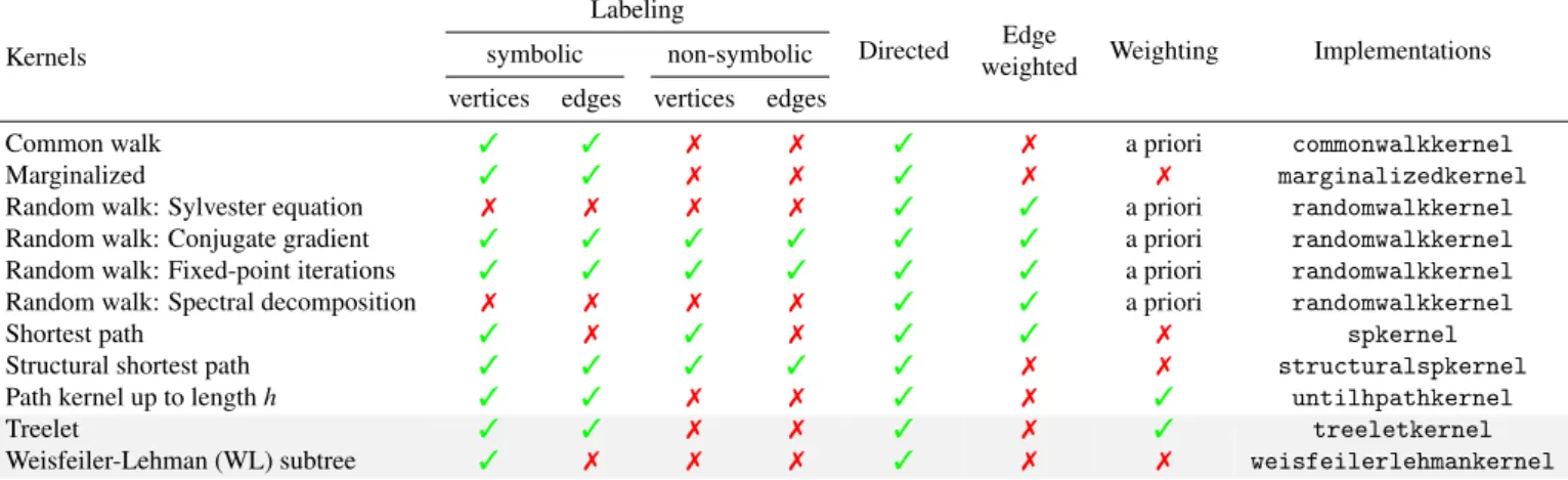
undirected graphs, and edge-weighted graphs. Only parts of these types have been tackled by other available libraries. Ta-ble 2 shows the types of graphs that each kernel can process.
Each kernel method takes a list of NetworkX graph objects as the input, and returns a Gram matrix whose entries are the evaluations of the kernel on pairs of graphs from the list. Other arguments can be chosen by the users to specify the computing methods and to serve as the tunable hyper-parameters of the kernel, according to the definition of the kernel. The compu-tation is then carried out with a single Python statement. The specific implementation of each graph kernel is described next. commonwalkkernel implements the common walk kernel. Two computing methods are provided based on exponential
se-Table 2. Comparison of graph kernels.
Kernels
Labeling
Directed Edge
weighted Weighting Implementations symbolic non-symbolic
vertices edges vertices edges
Common walk 3 3 7 7 3 7 a priori commonwalkkernel Marginalized 3 3 7 7 3 7 7 marginalizedkernel Random walk: Sylvester equation 7 7 7 7 3 3 a priori randomwalkkernel Random walk: Conjugate gradient 3 3 3 3 3 3 a priori randomwalkkernel Random walk: Fixed-point iterations 3 3 3 3 3 3 a priori randomwalkkernel Random walk: Spectral decomposition 7 7 7 7 3 3 a priori randomwalkkernel
Shortest path 3 7 3 7 3 3 7 spkernel
Structural shortest path 3 3 3 3 3 7 7 structuralspkernel Path kernel up to length h 3 3 7 7 3 7 3 untilhpathkernel
Treelet 3 3 7 7 3 7 3 treeletkernel
Weisfeiler-Lehman (WL) subtree 3 7 7 7 3 7 7 weisfeilerlehmankernel
“Weighting” indicates whether the substructures can be weighted in order to obtain a similarity measure adapted to a particular prediction task.
ries and geometric series as introduced by Gärtner et al. (2003). The direct product of labeled graphs is implemented for the convenience of computation.
marginalizedkernel computes the marginalized kernel with the recursion algorithm (Kashima et al., 2003). The users can set the argument remove_totters=True to remove totter-ing with the method introduced by Mahé et al. (2004).
The generalized random walk kernel is implemented by randomwalkkernel. Four possible computing methods are provided: Sylvester equation, conjugate gradient, fixed-point iterations, and spectral decomposition, as introduced by Vish-wanathan et al. (2010). The argument compute_method allows to select one of the four methods. For conjugate gradient and fixed-point iterations, the labels of vertices at the two ends of an edge are added to both sides of the corresponding edge labels.
The shortest path kernel is computed by spkernel. The Floyd-Warshall’s algorithm (Floyd, 1962) is employed to trans-form the original graphs into shortest-paths graphs (Borg-wardt and Kriegel, 2005). structuralspkernel computes the structural shortest path kernel introduced by Ralaivola et al. (2005). The Fast Computation of Shortest Path Kernel (FCSP) method is applied for both kernels. See Section 3.1 for details.
untilhpathkernel computes the path kernel up to length h. Two normalization kernels can be chosen, the Tanimoto ker-nel and the MinMax kerker-nel, studied by Suard et al. (2007). It is recommended to choose the trie data structure to store paths ac-cording to h and structure properties of graphs (see Section 3.3). Two graph kernels based on non-linear patterns are imple-mented: treeletkernel for the treelet kernel (Gaüzère et al., 2015b) and weisfeilerlehmankernel for the Weisfeiler-Lehman (WL) subtree kernel (Shervashidze et al., 2011).
Besides, user-defined vertex kernels and/or edge kernels of labeled graphs are supported in the shortest path kernels, the structural shortest path kernel, and the generalized random walk kernel computed by conjugate gradient and fixed-point it-erations methods. These kernels allow using simultaneously symbolic and non-symbolic labels in graph kernels, which en-ables graph kernels to tackle more types of graph datasets. The module utils.kernels contains several pre-defined ker-nels between labels of vertices or edges, in which the function
deltakernel computes the Kronecker delta function between symbolic labels, the function gaussiankernel computes the Gaussian kernel between non-symbolic labels, the function kernelsum and kernelproduct are respectively the sum and product of kernels between symbolic and non-symbolic labels. Moreover, edge weights can be included in the shortest path kernel, the structural shortest path kernel, and the generalized random walk kernel computed by Sylvester equation and spec-tral decomposition methods.
2.3. Model Selection and Evaluation
For the convenience of use, a complete model se-lection and evaluation procedure is implemented in the module gklearn.utils.model_selection_precomputed, in which all work is carried out by model_selection _for_precomputed_kernel. This method first preprocesses the input dataset, then computes Gram matrices and performs the model evaluation with machine learning methods from the scikit-learn library (Pedregosa et al., 2011). Support Vector Machines (SVM) are applied for classification tasks and kernel ridge regression for regression (Schölkopf and Smola, 2002). A two-layer nested cross-validation (CV) is applied to select and evaluate models, where the outer CV randomly splits the dataset into 10 folds with 9 as validation set, and the inner CV then ran-domly splits the validation set to 10 folds with 9 as training set. The whole procedure is performed 30 times, and the average performance is computed over these trails. The kernel param-eters are tuned within this procedure. This design allows the users to perform model selection in a single Python statement. Demos to use the library are provided in the notebooks folder.
3. Strategies to Reduce the Computation Complexity The computational complexity limits the practicability and scalability of graph kernels. In this section, we consider 3 strategies to reduce the computing time and memory usage to compute graph kernels: the Fast Computation of Shortest Path Kernel method, parallelization, and the trie structure. Datasets and environment settings applied in this section are described in Section 4.2.
are at most n1shortest paths in G1and n2shortest paths in G2,
thus n21n22comparisons between shortest paths and 2n21n22 com-parisons between vertices are required to compute the kernel. Each pair of vertices is compared 2n1n2times on average.
The Fast Computation of Shortest Path Kernel (FCSP) re-duces this redundancy (Xu et al., 2014). Instead of compar-ing vertices durcompar-ing the procedure of comparcompar-ing shortest paths, FCSP first compares all pairs of vertices between 2 graphs, and then stores the comparison results in an n1× n2matrix named
shortest path adjacency matrix; finally when comparing short-est paths, comparison results of corresponding vertices are re-trieved from the matrix. This method reduces vertex compar-isons to at most n1n2times, with an additional memory usage
of size O(n1n2). In practice, FCSP can reduce the time
com-plexity up to several orders of magnitudes.
In our implementation, we apply this vertex comparing method to the shortest path kernel, as recommended by Xu et al. (2014). Moreover, we also extend this strategy and apply it to the structural shortest path kernel, which allows reducing more redundancy since this kernel requires comparisons between all vertices on each pair of shortest paths. If the average length of the shortest paths in G1and G2is h, the new method is at most
n1n2htimes faster than direct comparison.
We further extend this strategy to edge comparison when computing the structural shortest kernel. If G1 has m1 edges
and G2has m2edges, then it requires m1m2times of edge label
comparisons, compared to n21n22htimes by the original method. 3.2. Parallelization
Parallelization may significantly reduce the computational complexity. The basic concept of parallelization is to split a set of computation tasks into several pieces, and then carry them out separately on multiple computation units such as CPUs or GPUs. We implement parallelization with Python’s multiprocessing.Pool module in two aspects: In cross-validation, parallelization is carried out over the set of trials; parallelization is performed on pairs of graphs when comput-ing Gram matrices of graph kernels (except for the WL subtree kernel due to the special structure of the kernel).
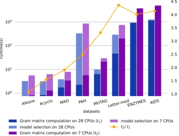
Many factors may influence the efficiency of parallelization, such as the number of computation cores, the transmission bandwidth between these cores, the method to split the data, the computational complexity to tackle one piece of data, etc. Fig. 2 reveals the influence of parallelization and CPU core numbers (7 versus 28), on runtime to compute Gram matrices and to perform model selections for the shortest path kernel on 8 datasets. Moreover, we present the ratio between runtimes to compute the Gram matrices on 28 and 7 cores. The values of this ratio for large-scale datasets are around 4, which turns out to be the inverse ratio of the number of CPU cores (28/7). It is
Alkane Acyclic MAO PAH MUTAGLetter-medENZYMES AIDS
datasets 100 101 1.0 1.5 2.0
Gram matrix computation on 28 CPUs (t1)
model selection on 28 CPUs Gram matrix computation on 7 CPUs (t2)
model selection on 7 CPUs t2/ t1
Fig. 2. Left y-axis: Runtimes (in seconds) to compute Gram matrices (bot-tom of each pillar) and perform model selections (top of each pillar) for the shortest path kernel on each dataset on 28 CPU cores (blue pillar) and 7 CPU cores (magenta pillar) with parallelization. Right y-axis: The or-ange dots are the ratios between the runtimes to compute Gram matrices of each dataset on 28 and 7 cores.
100 101 102 103 104 105 parallel chunksize 10−5 10−4 10−3 10−2 10−1 run tim e( s ) p er pa ir o f g rap hs Alkane
Acyclic MAOPAH MUTAGLetter-med ENZYMESAIDS
Fig. 3. Runtimes to compute the Gram matrices of the shortest path kernel on each dataset on 28 CPU cores with different chunksize values.
worth noting that the Letter-med dataset has the largest number of graphs (but with relatively “small” graphs), and Enzymes has the “average-largest” graphs (the second one being PAH).
Ideally, parallelization is more efficient when more compu-tation cores are applied. However, this efficiency may be sup-pressed by the parallel procedure required to distribute data to computation cores and collect returned results. Parallelizing relatively small graphs to a large number of computation cores may be more time consuming than non-parallel computation. For instance, Fig. 2 shows that it takes almost the same time to compute the Gram matrix of the small dataset Alkane on 28 and 7 CPU cores, indicating that the time efficiency raised by applying more CPU cores is nearly neutralized by the cost to allocate these cores. To tackle this problem, it is essential to choose an appropriate chunksize, which describes how many data are grouped together as one piece to be distributed to a single computation core.
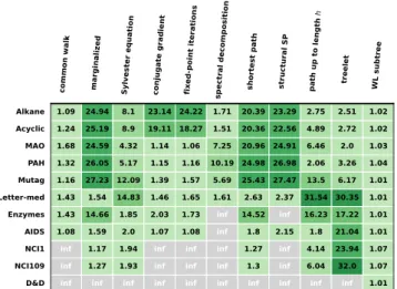
common walk marg inalize d Sylve ster e quati on conjug ate gr adien t fixed-p oint i te ration s sp ectra l dec omp ositi on sh orte st pa th struc tu ral S P pa th up to len gth h treele t WL su btree Alkane 1.09 24.94 8.1 23.14 24.22 1.71 20.39 23.29 2.75 2.51 1.02 Acyclic 1.24 25.19 8.9 19.11 18.27 1.51 20.36 22.56 4.89 2.72 1.02 MAO 1.68 24.59 4.32 1.14 1.06 7.25 20.96 24.91 6.46 2.0 1.03 PAH 1.32 26.05 5.17 1.15 1.16 10.19 24.98 26.98 2.06 3.26 1.04 Mutag 1.16 27.23 12.09 1.39 1.57 5.69 25.43 27.47 13.5 6.17 1.01 Letter-med 1.43 1.54 14.83 1.46 1.65 1.61 2.63 2.37 31.54 30.35 1.01 Enzymes 1.43 14.66 1.85 2.03 1.73 inf 14.52 inf 16.23 17.22 1.01 AIDS 1.08 1.59 2.0 1.07 1.08 inf 1.8 2.15 1.8 21.04 1.01 NCI1 inf 1.17 1.94 inf inf inf 1.27 inf 4.14 23.94 1.07 NCI109 inf 1.27 1.93 inf inf inf 1.3 inf 6.04 32.0 1.07 D&D inf inf inf inf inf inf inf inf inf inf 1.01 Fig. 4. The ratio between runtimes of the worse and the best chunksize settings for each graph kernel on each dataset. Darker color indicates a better result. Gray cells with the “inf” marker indicate that the compu-tation of the graph kernel on the dataset is omitted due to much higher consumption of computational resources than other kernels.
In Fig. 3, runtimes to compute the Gram matrices of the shortest path kernel with different chunksize values are com-pared on 28 CPU cores. When chunksizes are too small, the runtimes become slightly high, as the parallel procedure costs too much time; as chunksizes become bigger, the runtimes turn smaller, and then reach the minima; after that, the run-times may become much bigger as chunksizes continue grow-ing, due to the waste of computational resources. The mini-mum runtime of each dataset (shown with the vertical dot lines) varies due to the time and memory consumed to compute Gram matrices. Computations with wise chunksize choices could be more than 20 times faster than the worst choices. In our experiments, for convenience of implementations and compar-isons, the chunksize to compute an N × N Gram matrix on n♥
CPU cores is set to 100 if N2 > 100n
♥; and N2/n♥ otherwise.
The value 100 is chosen since the corresponding runtimes are close enough to their minima on all the datasets.
The ratio between runtimes of the worse and the best chunksize settings for each graph kernel on each dataset is shown in Fig. 4. On all available settings, the proper choices of the chunksizes speed up the computation. Some are more than 30 times faster than the worse chunksize settings (i.e., the path kernel up to length h and the treelet kernel on Letter-med). 3.3. The trie Structure
In some graph kernels that require comparison of paths (i.e., the path kernel up to h), the paths are pre-computed for the sake of time complexity. However, for large datasets, when the max-imum limits of the lengths of paths are high, storing these paths becomes memory consuming. Ralaivola et al. (2005) proposed a suffix tree data structure for fast computation of path kernels. Inspired by that, we employ the trie data structure (Fredkin, 1960) to store paths in order to tackle the memory problem.
The trie combines the common prefixes of paths together to reduce space complexity. Take the path kernel up to h for ex-ample. Let n be the average vertex number of each graph, d be
1 2 3 4 5 6 7 8 9 10 maximum length of paths h
102 103 104 105 106 107 me mo ry usa ge (K B) Alkane PAH ENZYMES NCI1 NCI109
Fig. 5. Memory usages to store paths in all graphs in each dataset under different maximum length of paths h. Dot lines represent explicit storage of paths, and solid lines represent storage using the trie structure. Note that lines of datasets NCI1 and NCI109 overlap.
Table 3. Experimental settings.
Environments Settings
CPU Intel(R) Xeon(R) E5-2680 v4 @ 2.40GHz
# CPU cores 28
Memory (in total) 252 GB
Operating system CentOS Linux release 7.3.1611, 64 bit
Python version 3.5.2
the average vertex degree, and l the different vertex labels in to-tal (for conciseness, only symbolic vertex labels are considered here). When paths are stored explicitly in memory (i.e., using the Python list object), the space complexity to store paths in one graph is in O(n(1+ d + · · · + dh)); The trie reduces it to
O(l(1+ l + · · · + lh)), making it very efficient for large datasets
and graphs, and when h is high. See Fig. 5 for a comparison. Although saving paths to the trie structure and retrieving paths from it require extra computing time, less memory us-age may avoid possible swapping between memory and hard disk, which may save more time in practice. As a result, the users should use trie structure according to the limits of their computing resources. In graphkit-learn, the trie structure is implemented for the path kernel up to h.
4. Experiments
To show the effectiveness and the practicability of the graphkit-learn library, we tested the library on synthesized graphs and several real-world datasets. A two-layer nested CV is applied to select and evaluate models, which is described in detail in Section 2.3. Table 3 summarizes the settings used in the experiments.
4.1. Performance on Synthesized Graphs
In this section, the performance and properties of each graph kernel are studied using synthesized graphs, with runtimes esti-mated on the Gram matrix computations.
First, we study the scalability of the kernels by increasing the number of graphs in the dataset (from 100 to 1000), where the
0.0 0.2 0.4 0.6 0.8 1.0 0.0 0.2 0.4 0.6 # of graphs # of vertices 2 4 6 8 10 degrees 100 101 102 103 104 105 run tim e( s ) (c) degrees 5 10 15 20 # of alphabets 100 101 102 run tim e( s )
(d) alphabet size of vertex labels
10 20 30 40 # of alphabets 5 10 15 20 25 run tim e( s )
(e) alphabet size of edge labels
datasets 0 20 40 60 80 100 ac cu rac y(% ) (f) degree dis%ribu%i ns en%r py ≈ 0.4 en%r py ≈ 2.2 c mm n (alk marginalized Sylves%er equa%i n c njuga%e gradien%
fi)ed-p in% i%era%i ns Spec%ral dec mp si%i n sh r%es% pa%h s%ruc%ural sp
pa%h up % leng%h h %reele% WL sub%ree
Fig. 6. Performance of all graph kernels on synthesized graphs.
generated unlabeled graphs consist of 20 vertices and 40 edges randomly assigned to pairs of vertices. Fig. 6(a) shows the run-times for all kernels. Since all the lines are linear with the y-axis being in square root scale, this indicates that the runtimes are quadratic in the number of graphs.
The scalability is also analyzed by increasing the number of vertices (from 10 to 100), where 10 datasets of 100 unlabeled graphs each were generated. The average degree of all gener-ated graphs is equal to 2 and the edges are randomly assigned to pairs of vertices. Fig. 6(b) shows the runtimes increasing in the numbers of vertices, for all kernel. The path kernel up to length hkernel and the WL subtree kernel have the best scalability.
To study the scalability of the kernels w.r.t. the average vertex degree, we generated unlabeled graphs consisting of 20 vertices with increasing degrees (from 1 to 10). The edges are randomly assigned to pairs of vertices. For each of the 10 degree values, we generated 100 graphs. Fig. 6(c) shows that most kernels have good scalability to the degrees, the worst being the treelet kernel, as the number of treelets in each graph increases rapidly with the degree.
To study the scalability of the kernels w.r.t. the alphabet sizes of symbolic vertex labels, we generated unlabeled graphs of 20 vertices and 40 edges randomly assigned to pairs of vertices. The vertices are symbolically labeled with increasing alpha-bet sizes, and the edges are unlabeled. For each alphaalpha-bet size
et al., 2003)), and the latter is caused by the reduced comparison between vertex labels through the shortest paths.
The scalability of the kernels w.r.t. the alphabet sizes of edge labels is studied in the same way, except that the edges are sym-bolically labeled with increasing alphabet sizes, and the vertices are unlabeled. For each alphabet size (0, 4, 8, . . . , 40), we gen-erated 100 graphs. According to Fig. 6(e), the runtimes of the path kernel up to path h increase with the alphabet sizes, caused by the aforementioned reason concerning the trie structures. In general, the influence of the alphabet size on the runtime is small for all kernels.
Finally, we studied the classification performances of the ker-nels on graphs with different amounts of entropy on degree dis-tributions. For this reason, we generated two sets of 200 graphs with 40 vertices. Graphs of the first set have low entropy on degree distributions, while graphs of the second set have high entropy (0.4 versus 2.2 on average). Each set has two classes, one consisting of half of the graphs with one label on vertices and the other class another label. A classification task is per-formed on each set using the SVM classifier, and the accuracy is evaluated. Fig. 6(f) shows that all graph kernels achieve equiv-alent accuracy on the both degree distributions. Except for the generalized random walk kernels computed by either Sylvester equation or spectral decomposition that cannot deal with labels, all graph kernels achieve high accuracy. It indicates that these graph kernels are suitable for various degree distributions.
As a conclusion, the dataset size and the number of vertices have the most significant effect on the computation runtimes of the aforementioned graph kernels. For the treelet kernel, the vertex degree is also important. These effects should be exam-ined carefully before using the kernels.
4.2. Real-world Datasets
In the following experiments, 11 well-known real-world datasets are considered for regression and classification tasks. These datasets come from different fields: Alkane (Cherqaoui and Villemin, 1994), Acyclic (Cherqaoui et al., 1994), MAO (Brun, 2018), PAH (Brun, 2018), Mutag (Debnath et al., 1991), Enzymes (Schomburg et al., 2004; Borgwardt et al., 2005), AIDS (Riesen and Bunke, 2008), NCI1 (Wale et al., 2008), NCI109(Wale et al., 2008) and D&D (Dobson and Doig, 2003) are chemical compounds and proteins from the bio /chemo-informatics fields; Letter-med (Riesen and Bunke, 2008) in-volves graphs of distorted letter drawings, within the category of image recognition. Alkane and Acyclic are concerned with the determination of the boiling point using regression. The other datasets are related to classification tasks. These datasets have a wide range of graph properties, by including labeled and unlabeled graphs, symbolic and non-symbolic attributes, di ffer-ent average vertex numbers, linear and non-linear patterns, etc.
common walk marg inaliz ed Sylve ster e quati on conjug ate gr adien t fixed-p oint i te ration s sp ectra l dec omp ositi on sh orte st pa th struc tu ral S P pa th up to len gth h treele t WL su btree Alkane 15.52 43.75 8.97 11.13 12.78 12.95 7.81 8.65 9.0 2.53 26.42 Acyclic 12.93 18.77 32.5 13.15 14.2 33.05 9.03 13.1 6.66 5.99 19.8 MAO 93.0 85.62 84.52 88.57 73.71 77.67 87.81 91.62 85.43 91.19 93.05 PAH 71.8 57.67 71.5 73.93 58.33 70.73 69.4 74.5 75.27 66.3 75.93 Mutag 85.96 76.11 82.77 86.18 86.58 84.05 81.84 86.26 88.47 90.79 87.18 Letter-med 36.16 5.2 37.27 93.12 91.3 36.38 93.72 94.88 43.83 inf 36.13 Enzymes 42.81 45.92 23.24 60.89 63.11 23.68 70.09 inf 57.49 52.23 50.76 AIDS 94.71 inf 92.42 98.93 98.57 87.21 99.26 98.84 99.65 99.54 98.63 NCI1 inf inf 59.76 71.34 inf inf inf 79.88 84.84 64.84 84.63 NCI109 inf inf 60.62 67.6 67.25 inf inf 79.04 83.94 63.46 85.47 D&D inf inf inf inf inf inf inf inf 81.4 inf 77.3 Fig. 7. Accuracy achieved by graph kernels, in terms of regression error (the upper table) and classification rate (the lower table). Red color in-dicates the worse results and dark green the best ones. Gray cells with the “inf” marker indicate that the computation of the graph kernel on the dataset is omitted due to much higher consumption of computational re-sources than other kernels.
The diversity of these particularities allows to explore the be-havior of the graph kernels on different types of graphs and the coverage of graphs that graphkit-learn is able to manage. See (Kersting et al., 2016) for details on these datasets. 4.3. Performance on the Real-world Datasets
Fig. 7 shows the accuracy achieved by the aforementioned graph kernels. Each row corresponds to a dataset and each column to a graph kernel. All kernels achieve better results compared with random assignment, where kernels based on paths and non-linear patterns outperform those based on walks on most datasets. Kernels based on paths achieve equivalent or even better results than those on non-linear patterns, where the path kernel up to length h dominates on most datasets with symbolic labels; while when non-symbolic labeled graphs are given, kernels based on shortest paths achieve the best results (such as Letter-med and Enzymes).
These results confirm graphkit-learn’s ability to tackle various types of graphs, which are labeled or unlabeled, with symbolic and/or symbolic attributes, linear and/or non-linear patterns, and have a wide range of average vertex num-bers from 4 (Letter-med) to 284 (D&D). Kernels based on linear patterns achieve competitive accuracies on graphs with non-linear patterns compared to kernels based on non-non-linear pat-terns. Along with the preceding analyses, these facts prove that these kernels can serve as reliable methods for classification and regression problems on graphs, as well as qualified benchmark kernels for future graph kernels design.
Besides accuracy, we furthermore examined the computa-tional complexity of each kernel. Fig. 8 displays the time con-sumed to compute the Gram matrix of each kernel on each dataset. The results are consistent with the computational com-plexities of graph kernels. In most cases, the computation is
common walk marg inalize d Sy lveste r equ ation conjug ate gr adien t fixed-p oint i teration s spec tral d ecomp os ition shor test path struc tura l SP path up to length h treele t WL su btree Alkane 0.48 0.51 -0.42 -0.18 -0.22 -0.19 -0.12 0.02 -0.29 -0.3 0.16 Acyclic 0.36 0.62 -0.18 -0.04 -0.11 -0.1 -0.08 0.24 -0.3 -0.31 0.34 MAO 0.81 0.69 -0.47 -0.11 -0.03 0.14 0.25 0.88 -0.14 -0.28 -0.25 PAH 1.56 1.05 -0.42 0.14 0.25 0.37 0.36 1.32 -0.28 -0.24 -0.03 Mutag 1.28 1.36 -0.3 0.44 0.53 0.77 0.69 1.84 -0.07 -0.24 0.19 Letter-med 2.01 2.08 1.13 1.97 1.85 1.78 1.57 1.62 1.08 inf 2.02 Enzymes 3.9 3.18 0.72 2.62 2.79 3.4 2.85 inf 2.16 2.08 1.41 AIDS 2.83 inf 1.37 2.91 3.03 3.74 2.95 3.9 1.59 0.87 2.22
NCI1 inf inf 2.3 3.96 inf inf inf 5.12 2.04 1.48 3.02
NCI109 inf inf 2.3 4.37 4.38 inf inf 5.13 2.05 1.48 1.48 D&D inf inf inf inf inf inf inf inf 2.67 inf 2.95 Fig. 8. Computational time to compute Gram matrices of graph kernels (in log10of seconds). Same color legends as Fig. 7 are used.
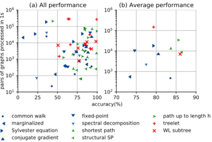
0.0 0.2 0.4 0.6 0.8 1.0 accuracy(%) 0.0 0.2 0.4 0.6 0.8 1.0 pa irs of gra ph s p roc esse d i n 1 s 0 25 50 75 100 101 102 103 104 105
106
(a) All performance
70 75 80 85 90 102 103 104 105 106
(b) Average performance
common walk marginalized Sylvester equation conjugate gradient fixed-point spectral decomposition shortest path structural SP path up to length h treelet WL subtreeFig. 9. Comparison of computational complexity versus accuracy of all graph kernels on all datasets (a), as well as the average performance of each kernel over all datasets (b). Markers correspond to different kernels; Colors blue, green and red depict graph kernels based on walks, paths and non-linear patterns, respectively.
efficient and it takes seconds or minutes to compute the whole Gram matrix. On the largest dataset (i.e., D&D, which contains 1178 graphs with 284 vertices and 715 edges per graph aver-age), two graph kernels can still be computed in tolerable time. For example, the path kernel up to length h can be computed within 8 minutes on D&D, which benefits from not only its rel-atively lower computational complexity, but also the trie struc-ture applied to it (see Section 3.3). Notice that it takes too much time to compute some graph kernels on some large datasets. For instance, the computational complexity of the common walk kernel is in O(n6) per pair of graphs. To this end, it is irrational
to apply this kernel on graphs with large amounts of vertices. In conclusion, these analyses illustrate the practicability of the graphkit-learn library.
The joint performance of the computational complexity and accuracy of each graph kernel on each dataset is shown in
5. Conclusion and Future Work
In this paper, we presented the Python library
graphkit-learn for graph kernel computations. It is the first library that provides a thorough coverage of graph kernels based on linear patterns (9 kernels based on linear patterns and 2 on non-linear patterns for comparison). We provided 3 strategies to reduce the computational complexity, including the extension of the FCSP method for other kernels and edge comparison. Experiments showed that it is easy to take advantage of the proposed library to compute graph kernels, in conjunction with the well-known scikit-learn library for Machine Learning. Future work includes imple-mentations of other non-linear kernels, a more thorough test of graph kernels on a wider range of benchmark datasets, a C++ implementation bound to Python interface for faster computation, and integrating more machine learning tools for graphs in the library, such as graph edit distance methods and tools to solve the graph pre-image problem. Meanwhile, we encourage interested users and authors of graph kernels to commit their implementations to the library.
Acknowledgments
This research was supported by CSC (China Scholarship Council) and the French national research agency (ANR) un-der the grant APi (ANR-18-CE23-0014). The authors would like to thank the CRIANN (Centre Régional Informatique et d’Applications Numériques de Normandie) for providing com-putational resources.
References
Borgwardt, K.M., Kriegel, H.P., 2005. Shortest-path kernels on graphs, in: Data Mining, Fifth IEEE International Conference on, IEEE. pp. 8–pp. Borgwardt, K.M., Ong, C.S., Schönauer, S., Vishwanathan, S., Smola, A.J.,
Kriegel, H.P., 2005. Protein function prediction via graph kernels. Bioinfor-matics 21, i47–i56.
Bougleux, S., Dupé, F.X., Brun, L., Mokhtari, M., 2012. Shape similarity based on a treelet kernel with edition, in: Gimel’farb, G., et al. (Eds.), Structural, Syntactic, and Statistical Pattern Recognition, Springer Berlin Heidelberg, Berlin, Heidelberg. pp. 199–207.
Brun, L., 2018. Greyc chemistry dataset. URL: https://brunl01.users. greyc.fr/CHEMISTRY/index.html. accessed October 30, 2018. Cherqaoui, D., Villemin, D., 1994. Use of a neural network to determine the
boiling point of alkanes. Journal of the Chemical Society, Faraday Transac-tions 90, 97–102.
Cherqaoui, D., Villemin, D., Mesbah, A., Cense, J.M., Kvasnicka, V., 1994. Use of a neural network to determine the normal boiling points of acyclic ethers, peroxides, acetals and their sulfur analogues. Journal of the Chemical Society, Faraday Transactions 90, 2015–2019.
Gärtner, T., Flach, P., Wrobel, S., 2003. On graph kernels: Hardness results and efficient alternatives. Learning Theory and Kernel Machines , 129–143. Gaüzère, B., Brun, L., Villemin, D., 2012. Two new graphs kernels in
chemoin-formatics. Pattern Recognition Letters 33, 2038–2047.
Gaüzère, B., Brun, L., Villemin, D., 2015a. Graph kernels in chemoinformatics, in: Dehmer, M., Emmert-Streib, F. (Eds.), Quantitative Graph Theory Math-ematical Foundations and Applications. CRC Press, pp. 425–470. URL: https://hal.archives-ouvertes.fr/hal-01201933.
Gaüzère, B., Grenier, P.A., Brun, L., Villemin, D., 2015b. Treelet kernel incor-porating cyclic, stereo and inter pattern information in chemoinformatics. Pattern Recognition 48, 356 – 367.
Ghosh, S., Das, N., Gonçalves, T., Quaresma, P., Kundu, M., 2018. The journey of graph kernels through two decades. Computer Science Review 27, 88– 111.
Hagberg, A., Swart, P., S Chult, D., 2008. Exploring network structure, dynam-ics, and function using NetworkX. Technical Report. Los Alamos National Lab.(LANL), Los Alamos, NM (United States).
Kashima, H., Tsuda, K., Inokuchi, A., 2003. Marginalized kernels between labeled graphs, in: Proceedings of the 20th international conference on ma-chine learning (ICML-03), pp. 321–328.
Kersting, K., Kriege, N.M., Morris, C., Mutzel, P., Neumann, M., 2016. Benchmark data sets for graph kernels. URL: http://graphkernels. cs.tu-dortmund.de.
Kriege, N.M., Neumann, M., Morris, C., Kersting, K., Mutzel, P., 2019. A unifying view of explicit and implicit feature maps of graph kernels. Data Mining and Knowledge Discovery 33, 1505–1547.
Mahé, P., Ueda, N., Akutsu, T., Perret, J.L., Vert, J.P., 2004. Extensions of marginalized graph kernels, in: Proceedings of the twenty-first international conference on Machine learning, ACM. p. 70.
Morris, C., Kersting, K., Mutzel, P., 2017. Glocalized weisfeiler-lehman graph kernels: Global-local feature maps of graphs, in: 2017 IEEE International Conference on Data Mining (ICDM), pp. 327–336.
Pedregosa, F., Varoquaux, G., Gramfort, A., Michel, V., Thirion, B., Grisel, O., Blondel, M., Prettenhofer, P., Weiss, R., Dubourg, V., Vanderplas, J., Passos, A., Cournapeau, D., Brucher, M., Perrot, M., Duchesnay, E., 2011. Scikit-learn: Machine learning in Python. Journal of Machine Learning Research 12, 2825–2830.
Ralaivola, L., Swamidass, S.J., Saigo, H., Baldi, P., 2005. Graph kernels for chemical informatics. Neural networks 18, 1093–1110.
Riesen, K., Bunke, H., 2008. Iam graph database repository for graph based pat-tern recognition and machine learning, in: Joint IAPR Inpat-ternational Work-shops on Statistical Techniques in Pattern Recognition and Structural and Syntactic Pattern Recognition, Springer. pp. 287–297.
Schölkopf, B., Smola, A.J., 2002. Learning with kernels: support vector ma-chines, regularization, optimization, and beyond. MIT press.
Schomburg, I., Chang, A., Ebeling, C., Gremse, M., Heldt, C., Huhn, G., Schomburg, D., 2004. Brenda, the enzyme database: updates and major new developments. Nucleic acids research 32, D431–D433.
Shervashidze, N., Schweitzer, P., Leeuwen, E.J.v., Mehlhorn, K., Borgwardt, K.M., 2011. Weisfeiler-lehman graph kernels. Journal of Machine Learning Research 12, 2539–2561.
Suard, F., Rakotomamonjy, A., Bensrhair, A., 2007. Kernel on bag of paths for measuring similarity of shapes., in: ESANN, pp. 355–360.
Vishwanathan, S.V.N., Schraudolph, N.N., Kondor, R., Borgwardt, K.M., 2010. Graph kernels. Journal of Machine Learning Research 11, 1201–1242. Wale, N., Watson, I.A., Karypis, G., 2008. Comparison of descriptor spaces for
chemical compound retrieval and classification. Knowledge and Information Systems 14, 347–375.
Xu, L., Wang, W., Alvarez, M., Cavazos, J., Zhang, D., 2014. Parallelization of shortest path graph kernels on multi-core cpus and gpus. Proceedings of the Programmability Issues for Heterogeneous Multicores (MultiProg), Vienna, Austria .
Appendix A. Examples to Use the Library
In this appendix we show usage examples of the library. The dataset MUTAG and the path kernel up to length h are used as the example.
First, a single Python statement allows to load a graph dataset:
1 f r o m g k l e a r n . u t i l s . g r a p h f i l e s i m p o r t l o a d D a t a s e t
2
3 graphs , t a r g e t s = l o a d D a t a s e t (’ D A T A _ F O L D E R / M U T A G /
M U T A G _ A . txt ’)
“DATA_FOLDER” is the user-defined folder to store the datasets. With the loaded graphs, the Gram matrix can be computed as following: 1 f r o m g k l e a r n . k e r n e l s i m p o r t u n t i l h p a t h k e r n e l 2 3 g r a m _ m a t r i x , r u n _ t i m e = u n t i l h p a t h k e r n e l ( 4 graphs , # The l i s t of i n p u t g r a p h s . 5 d e p t h =5 , # The l o n g e s t l e n g t h of p a t h s . 6 k _ f u n c =’ M i n M a x ’, # Or ’ t a n i m o t o ’. 7 c o m p u t e _ m e t h o d =’ t r i e ’, # Or ’ n a i v e ’. 8 n _ j o b s =1 , # The n u m b e r of j o b s to run in p a r a l l e l . 9 v e r b o s e = T r u e )
The Gram matrix and the time spent to compute it are returned. Besides kernel computation, a complete model selection and evaluation procedure using a 2-layer nested cross-validation can be performed by the following code:
1 f r o m g k l e a r n . u t i l s i m p o r t m o d e l _ s e l e c t i o n _ f o r _ p r e c o m p u t e d _ k e r n e l 2 f r o m g k l e a r n . k e r n e l s i m p o r t u n t i l h p a t h k e r n e l 3 i m p o r t n u m p y as np 4 5 # Set p a r a m e t e r s . 6 d a t a f i l e = ’ D A T A _ F O L D E R / M U T A G / M U T A G _ A . txt ’ 7 p a r a m _ g r i d _ p r e c o m p u t e d = { 8 ’ d e p t h ’: np . l i n s p a c e (1 , 10 , 10) , 9 ’ k _ f u n c ’: [’ M i n M a x ’, ’ t a n i m o t o ’] , 10 ’ c o m p u t e _ m e t h o d ’: [’ t r i e ’]} 11 p a r a m _ g r i d = {’ C ’: np . l o g s p a c e ( -10 , 10 , num =41 , b a s e = 1 0 ) } 12 13 # P e r f o r m m o d e l s e l e c t i o n and c l a s s i f i c a t i o n . 14 m o d e l _ s e l e c t i o n _ f o r _ p r e c o m p u t e d _ k e r n e l ( 15 d a t a f i l e , # The p a t h of d a t a s e t f i l e . 16 u n t i l h p a t h k e r n e l , # The g r a p h k e r n e l u s e d for e s t i m a t i o n . 17 p a r a m _ g r i d _ p r e c o m p u t e d , # The p a r a m e t e r s u s e d to c o m p u t e g r a m m a t r i c e s . 18 p a r a m _ g r i d , # The p e n e l t y P a r a m e t e r s u s e d for p e n e l t y i t e m s . 19 ’ c l a s s i f i c a t i o n ’, # Or ’ r e g r e s s i o n ’. 20 N U M _ T R I A L S =30 , # The n u m b e r of the r a n d o m t r i a l s of the o u t e r CV l o o p . 21 d s _ n a m e =’ M U T A G ’, # The n a m e of the d a t a s e t . 22 n _ j o b s =1 , 23 v e r b o s e = T r u e )
The “param_grid_precomputed” and the “param_grid” ar-guments specify grids of hyper-parameter values used for grid search in the cross-validation procedure. The results will be automatically saved.
More demos and examples can be found in the notebooks directory and the gklearn.examples module of the library.