HAL Id: hal-01370557
https://hal.inria.fr/hal-01370557
Submitted on 22 Sep 2016
HAL is a multi-disciplinary open access
archive for the deposit and dissemination of
sci-entific research documents, whether they are
pub-lished or not. The documents may come from
teaching and research institutions in France or
abroad, or from public or private research centers.
L’archive ouverte pluridisciplinaire HAL, est
destinée au dépôt et à la diffusion de documents
scientifiques de niveau recherche, publiés ou non,
émanant des établissements d’enseignement et de
recherche français ou étrangers, des laboratoires
publics ou privés.
Sai Qian, Philippe de Groote, Maxime Amblard
To cite this version:
Sai Qian, Philippe de Groote, Maxime Amblard. Modal Subordination in Type Theoretic Dynamic
Logic. Linguistic Issues in Language Technology, Stanford Calif.: CSLI Publications, 2016, Modes of
Modality in NLP, 14 ((1)), pp.1-39. �hal-01370557�
Modal Subordination in Type Theoretic
Dynamic Logic
Sai Qian, Institute of Energy, Jiangxi Academy of Sciences, China Philippe de Groote, INRIA Nancy Grand-Est, France Maxime Amblard, Université de Lorraine, LORIA, INRIA Nancy
Grand-Est, CNRS, UMR 7503, France
Abstract
Classical theories of discourse semantics, such as Discourse Represen-tation Theory (DRT), Dynamic Predicate Logic (DPL), predict that an indefinite noun phrase cannot serve as antecedent for an anaphor if the noun phrase is, but the anaphor is not, in the scope of a modal expression. However, this prediction meets with counterexamples. The phenomenon modal subordination is one of them. In general, modal subordination is concerned with more than two modalities, where the modality in subsequent sentences is interpreted in a context ‘subordi-nate’ to the one created by the first modal expression. In other words, subsequent sentences are interpreted as being conditional on the sce-nario introduced in the first sentence. One consequence is that the anaphoric potential of indefinites may extend beyond the standard lim-its of accessibility constraints.
This paper aims to give a formal interpretation on modal subordi-nation. The theoretical backbone of the current work is Type Theo-retic Dynamic Logic (TTDL), which is a Montagovian account of dis-course semantics. Different from other dynamic theories, TTDL was built on classical mathematical and logical tools, such as -calculus and Church’s theory of types. Hence it is completely compositional and does not suffer from the destructive assignment problem. We will review the basic set-up of TTDL and then present Kratzer’s theory on natural language modality. After that, by integrating the notion of
versation background, in particular, the modal base usage, we offer an extension of TTDL (called Modal-TTDL, or M-TTDL in short) which properly deals with anaphora across modality. The formal relation be-tween Modal-TTDL and TTDL will be discussed as well.
1 Modal Subordination
1.1 Dynamic SemanticsAround the middle of the last century, Alfred Tarski investigated the semantics of formal languages by defining the notion of truth (Tarski, 1944, 1956). Later on in the 1970s, his student Richard Montague es-tablished a model-theoretic semantics for natural language (Montague, 1970b,a, 1973) by using the mathematic tools of that time, e.g., higher-order predicate logic, -calculus, type theory, intensional logic, etc. This work is known as the Montague Grammar (MG), which makes the pos-sibility to interpret natural language, in particular English, as a formal language. Under MG, linguistic expressions are interpreted in terms of their contributions to the truth conditions of the sentences where they occur. This is recognized as the static view on meaning. Despite its pre-vailing influence in the field of logical semantics, MG was designed to account for the meaning of isolated sentences. Thus, linguistic phenom-ena that cross sentence boundaries, such as inter-sentential anaphora, donkey anaphora, presupposition, etc., lack proper explanations in MG. Since the 1980s, in order to overcome the empirical problems arising from MG, a number of semantic theories have been established from the discourse perspective. Representative works include Discourse Repre-sentation Theory (DRT) (Kamp, 1981), File Change Semantics (FCS) (Heim, 1982), and Dynamic Predicate Logic (DPL) (Groenendijk and Stokhof, 1991). In contrast with classical logical semantics such as MG, these theories are subsumed under the label dynamic semantics, where the meaning of a linguistic expression is identified with its potential to change the context, rather than the truth conditions. More specif-ically, the meaning of a sentence is the change it brings about to an existing discourse where it occurs; the meaning of a non-sentential ex-pression equals its contribution to that change. Summarized in a slogan, meaning is the “context change potential” (Heim, 1983). The no-tion of context in dynamic semantics denotes what gets changed during the interpretation. It is subject to the particular domain of research. For instance, when analyzing anaphoric relations between noun phrases and pronominal anaphors, the context resides in the discourse referents which have been introduced, namely the objects being talked about, and the possibilities that they are to be retrieved by anaphoric terms
in subsequent discourse.
Per contrast to static semantics, the above mentioned dynamic the-ories manage to give an account for the inter-sentential anaphora and donkey anaphora. At the same time, they help to constrain a number of infelicitous anaphors as well. Take the following discourses:
(1) Bill doesn’t have a cari. *Iti is black. (Karttunen, 1969)
(2) a. *Either Jones owns a bicyclei, or iti’s broken.
b. Jane either borrowed a cari or rented a truckj to get to
Boston. *Iti/j broke down on the way. (Simons, 1996)
(3) Every mani walks in the park. *Hei whistles. (Groenendijk and
Stokhof, 1991)
As indicated in each example, all anaphoric relations are problem-atic, and these anomalies can be correctly captured in dynamic seman-tics. According to the classical dynamic frameworks, negation blocks the accessibility of discourse referents within its scope, which explains example (1); disjunction blocks the accessibility of discourse referents from either disjunct, as well as from outside its scope, which explains example (2); and implication admits the accessibility of discourse ref-erents in the antecedent from the consequent, but not from outside its scope, which explains example (3).
1.2 Anaphora under Modality
Although the well-established constraints in dynamic semantics can ac-count for a wide range of empirical data concerning the accessibility of discourse anaphora, there are a number of exceptional linguistic exam-ples, where the life-span of a discourse referent is longer than expected. The perspective of this section is to sketch one specific case: modal subordination, which is also the main problem that we are trying to investigate in the current paper.
At first glance, modality has a similar effect as negation in blocking discourse referent. That is to say, if an indefinite noun phrase (NP) occurs in the scope of some modal operator, e.g., must, can, shall, etc., its discourse referent cannot be anaphorically linked to expressions in subsequent discourse. For instance:
(4) a. You must write a letterito your parents. *They are
expect-ing the letteri.
b. Bill can make a kitei. *The kitei has a long string.
(Kart-tunen, 1969)
letter and the kite, can refer back to the corresponding indefinite NP. That is because both indefinites are located in the complement clauses governed by model auxiliaries, i.e., must in (4-a), can in (4-b). To ac-count for examples as such in dynamic semantics, a basic strategy is to integrate two modal logic operators, namely the possibility operator 3 and the necessity operator 2, in the syntactic and semantic systems of the original theories. Modal operators are treated in a similar way as negation, which blocks discourse referents within its scope. We will not go further into this point since it is not the focus of the current paper. Despite the observation drawn from example (4), the following data suggest that anaphoric references are not always impossible across modality.
(5) If John bought a booki, he’ll be home reading iti by now. Iti’ll
be a murder mystery. (Roberts, 1989)
(6) A thiefi might break into the house. Hei would take the silver.
(Roberts, 1989)
In both above examples, the anaphoric expressions, namely the sec-ond it in (5) and he in (6), are interpreted as depending on the in-definites introduced under preceding modalities. These examples are different from (4) in the sense that the second sentences are not in the factual mood, rather, they contain modals of their own. Furthermore, in each case of (5) and (6), the modal in the second sentence is inter-preted in a context ‘subordinate’ to that created by the first modal. In other words, successive non-factual discourse is interpreted as being conditional on the scenario introduced in the first sentence. Standard dynamic frameworks fail to give an explanation of examples of this sort no discourse referent can survive outside the scope of modal operators. This phenomenon, where the accessibility barriers assumed in classical dynamic semantics are broken down by continuous modals, is known as modal subordination (Roberts, 1987, 1989).
To account for such examples (5) and (6), Roberts combines Kratzer’s theory of modality and DRT, where the blocked discourse referents are made available by repeating the whole sub-DRS into the DRS of the subordinate modal. However, Robert’s approach is not completely satis-factory. On the one hand, although this combination is straightforward, it has to be accompanied with several constraints. Otherwise, this ap-proach, namely accommodation of antecedent, is too powerful so it overgenerates and predicts that all referents introduced under modal-ity will be accessible to subsequent discourse. On the other hand, the
classical theory DRT is often criticized for lacking compositionality1.
Furthermore, it suffers from the so-called destructive assignment prob-lem. Hence, we will try to resolve the modal subordination problem based on a more recently proposed dynamic theory.
In the following section, we introduce the theoretical foundation of the current paper, namely Type Theoretic Dynamic Logic. In section 3, we present some preliminary notions on natural language modality, as well as a now classical theory about modality in the linguistic per-spective. Next, section 4 will focus on presenting our specific solution of modal subordination. Finally, in the last section we will delete out some general conclusions and further suggestions.
2 Type Theoretic Dynamic Logic
Around a decade ago, de Groote proposed a new dynamic framework Type Theoretic Dynamic Logic (TTDL) (de Groote, 2006). This framework aims to study the semantics of sentences and discourses in a uniform and classical way. In order to achieve dynamics, TTDL inte-grates the notion of left and right contexts into MG: given a sentence, its left context denotes the discourse that precedes it, namely what has already been processed; its right context is the continuation (Strachey and Wadsworth, 1974), denoting the discourse that follows it, namely what will be processed in future. A sentence is interpreted with respect to both its left and right contexts, and its semantics is abstracted over the two contexts.
Technically, TTDL sticks to the tradition of MG. It only makes use of standard mathematical and logical tools, such as -calculus and theory of types. Logical notions such as free and bound variables, quantifier scopes, are as usual. And the only operations involved are standard ↵-conversions and -reductions. This property enables it to inherit all nice properties of well-established mathematics and logics. In what follows, we present the formal details of TTDL.
Akin to other systems based on the simply typed -calculus, the syntax of TTDL can be defined in terms of the notion of higher order signature (de Groote, 2001), which is a triplet consisting of a finite set of atomic types, a finite set of constant symbols, and a function that assigns each constant a type.
Definition 2.1. The signature of TTDL, in notation ⌃T T DL, is defined
1The notion of compositionality has been successfully integrated in some later
as follows: ⌃T T DL=h{◆, o, }, {>, ^, ¬, 9, :: , sel, nil}, {> : o, ^ : o ! o ! o, ¬ : o ! o, 9 : (◆ ! o) ! o, :: : ◆ ! ! , sel : ! ◆, nil : }i
Logical constants such as > (tautology), ^ (conjunction), ¬ (nega-tion) and 9 (existential quantifier) are exactly the same as in First Order Logic (FOL). However, besides the two atomic types in Church’s simple type theory (Church, 1940): ◆ denoting the type of individuals and o denoting the type of propositions, there is a third one in TTDL: denoting the type of left contexts. The right context, which is in-terpreted as the continuation of the sentence, is a function from left contexts to truth values. So its type is ! o. For instance, assume e is a left-context variable, then the empty right context can be defined in the compact term stop as follows:
stop, e.> (2.1)
In order to solve pronominal anaphora in TTDL, the left context is modeled as a list of individuals. This explains the type of the empty context “nil” in ⌃T T DL. In addition to that, two operators are
intro-duced in definition 2.1. The first is the list constructor “::”. Its function is to add new individuals (of type ◆) into existing contexts (of type ). Hence the type of “::” is ◆ ! ! . The second is the choice operator “sel”, it takes a left context (of type ) as argument and yields back an individual (of type ◆). Hence its type is ! ◆.
In standard truth-conditional semantics, a sentence expresses a proposition, which is of type o. While in TTDL, a sentence will be interpreted with respect to both its left and right contexts, which are of type and ! o, respectively. If we use s to denote the syntactic category of sentences, J KT T DL to denote the semantic interpretation
under TTDL, then:
JsKT T DL= ! ( ! o) ! o (2.2)
Discourses, which also express propositions, are interpreted in the same way as single sentences. So, letting d be the syntactic category of discourses, we have:
JdKT T DL= ! ( ! o) ! o (2.3)
In order to contrast with o, which is the type of (standard/static) propositions, we call ! ( ! o) ! o the type of dynamic
proposi-tions. Hereinafter, we will use ⌦ as an abbreviation for ! ( ! o) ! o, namely:
⌦, ! ( ! o) ! o (2.4)
After presenting the typing information in TTDL, let us proceed to the logics of the framework. Let A and B be variables denoting dynamic propositions, e and e0 be variables denoting left contexts,
be a variable denoting the right context, then the dynamic conjunction ^d
T T DL in TTDL, which conjoins two dynamic propositions, is defined
as follows2:
^d
T T DL, ABe .Ae( e0.Be0 ) (2.5)
In the above formula, e and are the left and right contexts of the conjunction, they are also called the current left and right contexts. Formula 2.5 can be further elaborated as follows. First of all, the se-mantics of a conjunction is contributed by both conjuncts, this explains why A and B are both involved in the composition. In addition, the left context of the first conjunct is the current left context, this is why eis passed to A; the right context of the second conjunct is the current right context, this is why is passed to B. Finally, the right context of the first conjunct is made up of the second conjunct and the current right context, this explains why e0.Be0 is passed to A; the left
con-text of the second conjunct is made up of the first conjunct and the current left context, this explains why e0, which forms a -abstraction
and will be substituted by a complex structure of type (consisting of eand information in A), is passed to B.
In order to negate dynamic propositions, TTDL defines the dynamic negation operator ¬d
T T DL as follows:
¬dT T DL, Ae .¬(A e stop) ^ e (2.6)
where stop was defined in formula 2.1. The operator ¬d
T T DL takes a
dynamic proposition A and returns its dynamically negated counter-part, hence it is of type ⌦ ! ⌦. The right hand side of formula 2.6 can be further understood as follows. Firstly, the left context of the to-be-negated proposition A is the current left context, this is why e is passed to A. Furthermore, we do not want negation to take scope over any future part of the discourse, so the empty right context stop, rather than the current right context , is passed to A. Finally, a dy-namic negation does not have the potential to update the left context, this is why e, the function-application of the original left and right contexts, appears as a conjunct at the end of the formula.
2The conjunction we define here is for propositions only, it is hence not related
As to the dynamic existential quantifier in TTDL, it is defined as: 9dT T DL, Pe .9( x.Px(x :: e) ) (2.7)
The dynamic quantifier 9d
T T DLtakes a dynamic property P of type
◆ ! ⌦, and returns a existentially quantified dynamic proposition. Hence the semantic type of the operator 9d
T T DL is (◆ ! ⌦) ! ⌦.
The right hand side of formula 2.7 can be understood as follows. In an existentially quantified dynamic proposition, variables which are bound by the existential quantifier shall update the current left context, this is why the updated context (x :: e) is passed to the proposition within the scope of 9.
Above we have presented the dynamic logic in TTDL, in particular, the definitions of the dynamic operators. In fact, there exists a system-atic translation, which associates (standard/stsystem-atic) logical expressions to their dynamic counterparts. The translation process is concerned with both types and -terms, which will be examined one by one be-low.
Notation 2.1. We use the bar notation, for instance, ⌧ or M, to denote the dynamic translation of a type ⌧ or a -term M in TTDL.
Definition 2.2. The dynamic translation of a type ⌧: ⌧, is defined inductively as follows:
1. ◆ = ◆; 2. o = ⌦;
3. ! ⌧ = ! ⌧, where ⌧ and are types.
According to definition 2.2, the static and dynamic types of individ-uals are both ◆, while the static and dynamic type of propositions are o and ⌦, respectively. The dynamic translation of a function type is still a function type, with the argument type and the result type being translated respectively.
The dynamic translation of -terms will ground on the following two functions: the dynamization function D and the staticization func-tion S, whose definifunc-tions are mutually dependent. They will be used to translate non-logical constants.
Definition 2.3. The dynamization function D⌧, which takes an input
-term A of type ( ! ⌧), returns an output -term A0 of type ⌧; the
staticization function S⌧, which takes an input -term A0 of type ⌧,
returns an output -term A of type ( ! ⌧). D⌧ is defined inductively on type ⌧ as follows:
1. D◆A = A nil;
3. D↵! A = x.D ( e.Ae(S↵xe)).
S⌧ is defined inductively on type ⌧ as follows:
1. S◆A0= e.A0;
2. SoA0= e.A0 estop;
3. S↵! A0= e.( x.S (A0(D↵( e0.x)))e).
Now based on definition 2.3, we can proceed to the dynamic trans-lation of -terms.
Definition 2.4. The dynamic translation of a -term M (of type ⌧): M, which is another -term of type ⌧, is defined as follows:
1. x = x, if x is a variable;
2. a = D⌧( e.a), if a is a non-logical constant and a : ⌧;
3. ^ = ^d T T DL, see formula 2.5; 4. ¬ = ¬d T T DL, see formula 2.6; 5. 9 = 9d T T DL, see formula 2.7; 6. (MN) = (M N); 7. ( x.M) = ( x.M).
The dynamic counterparts of the derived operators, such as _ (dis-junction), ! (implication), and 8 (universal quantifier), are defined in terms of primitive logical constants and the corresponding rules in def-inition 2.4. Since the semantics of TTDL is almost the same as the one of FOL, we will not dig into that. Illustrations of TTDL will not be presented here for reasons of space. For more examples, please refer to (de Groote, 2006) and (Lebedeva, 2012).
With the above set-up, TTDL manifests the same empirical coverage on discourse anaphora as other dynamic frameworks, such as DRT and DPL. In the following section, we will first discuss modality in more detail from the linguistic perspective. Then we will present the theory of modality developed by Angelika Kratzer (Kratzer, 1977, 1981, 1986, 1991). After that in section 4, we shall combine Kratzer’s theory of modality with TTDL, yielding an adaptation of TTDL called Modal TTDL (M-TTDL), which treats the modal subordination problem in traditional montagovian style. A formal link between the new adapta-tion and TTDL will be established as well.
3 Preliminary Notions on Modality
3.1 Modality in Natural Language SemanticsGenerally speaking, modality is a semantic notion which is concerned with possibility and necessity. In linguistics, modality enables people to talk about things beyond the actual here and now (von Fintel, 2006).
It is reflected in the set of phenomena that express notions such as belief, attitude and obligation in natural language sentences. Modality, which has been pervasively attested across almost all languages, can be established by a wide range of grammatical categories and construc-tions. Take English for example, there are modal auxiliaries (e.g., must, may, should, might), modal adjective and adverbs (e.g., it is possible ..., possibly, necessarily, probably), conditionals (e.g., if ... then ...), propositional attitude verbs (e.g., believe, know, hope), etc.
One aspect of the semantics of modality is modal force, namely the strength of a modal, i.e., possibility and necessity. The two cor-responding operators are treated as quantifiers ranging over possible worlds: 3 as existential, 2 as universal. Because of that, possibility and necessity are also called existential force and universal force (respectively). The force of a modal expression is inherently contained in its lexical meaning. For instance, modals such as may, might and could always denote a possibility; while modals such as must, should and would always denote a necessity one.
Another aspect on the semantics of modality is modal flavor, it indicates the particular sort of premise information, e.g., epistemic, deontic, etc., with respect to which a modal is interpreted. This no-tion is motivated by the fact that it is insufficient to interpret modal expressions only relative to their modal forces. According to modal fla-vor, modalities can be classified into different sub-types. Let’s take the following sentences for example, where the modal is considered to be ambiguous:
(7) a. All Maori children must learn the names of their ancestors. b. The ancestors of the Maoris must have arrived from Tahiti.
(Kratzer, 1977)
Both (7-a) and (7-b) contain the same modal must, so each of them expresses a universal force. However, the meaning of must varies from one sentence to another. For instance, in (7-a), the modal must refers to an obligation or a duty that the Maori children should obey or fulfill, it is called a deontic modality; in (7-b), the same modal denotes some knowledge or belief, it is called an epistemic modality. This distinction can be revealed in an explicit way by paraphrasing (7) as follows, where an in view of ... adverbial phrase is added at the beginning of each sentence:
(8) a. In view of what their tribal duties are, the Maori children must learn the names of their ancestors.
have arrived from Tahiti. (Kratzer, 1977)
The modal must in (7-a) means “necessary in view of what their tribal duties are”; while must in (7-b) means “necessary in view of what is known”. A similar contrast can be found in the following examples: (9) a. According to his dating coach, John must dance at parties.
b. Since John hangs out with Linda at parties, he must dance at parties. (Starr, 2012)
By only looking at the modalized sentence John/he must dance at parties, which is shared by both discourses in (9), we are not able to tell whether it refers to an obligation (deontic), or a piece of knowledge (epistemic), or maybe something else. However, with the help of the prefixed adverbial phrases in (9), we can unambiguously determine that the shared modalized sentence expresses a deontic modality in (9-a), while it expresses an epistemic one in (9-a).
Actually, besides the deontic and epistemic modality as we have shown in the above examples, there are also other types of modality that a modal expression can express, such as bouletic (wishes or de-sires), teleological (goals), circumstantial (circumstances), etc., all of which are called the flavor of a modal3. For instance, all the
follow-ing examples involve the same modal expression have to, but denotes different modalities:
(10) a. It has to be raining. [after observing people coming inside with wet umbrellas; epistemic modality]
b. Visitors have to leave by six pm. [hospital regulations; de-ontic]
c. You have to go to bed in ten minutes. [stern father; bouletic]
d. I have to sneeze. [given the current state of one’s nose; circumstantial]
e. To get home in time, you have to take a taxi. [telelological] (von Fintel, 2006)
For more examples, please refer to (Kratzer, 1977, Portner, 2009). Different from the modal force, which solely comes from the lexical meaning of a modal, the modal flavor depends on the specific situation where the modal is applied. Sometimes, it is given by linguistic means, where there are noticeable indicators such as the adverbial phrases in view of ... and according to ... in (8) and (9); most of the time however,
no indicators are explicitly presented and the readers have to resolve the most appropriate flavor based on clues from the context of use, for instance, as in (7) and (10).
In order to interpret modal expressions in formal systems such as Modal Predicate Logic (MPL), we need to correctly handle both above mentioned semantic aspects. The treatment of modal force is relatively straightforward: 3 is the existential quantifier over possible worlds, 2 is the universal quantifier over possible worlds. As to modal flavor, what we can do is to assign each different modal a different set of possible worlds which it quantifies over. In other words, to associate each modal a corresponding accessibility relation4. However, from a
generalization point of view, this strategy is not satisfactory. In the next section, we will sketch Kratzer’s theory on modality, which aims to give a unified analysis on different types of modality (e.g., epistemic, deontic, bouletic, etc.).
3.2 Kratzer’s Theory of Modality
Currently, Kratzer’s theory of modality (Kratzer, 1977, 1981, 1986, 1991) is the most studied work in this field. It has served as the foun-dation for a large number of subsequent works on modality. One of the most essential motivations of Kratzer is to tackle the problem of lexical ambiguity among modals, providing a uniform treatment to modals of various modal forces.
In her theory, Kratzer proposes that modals are context-dependent, rather than ambiguous between various flavors. As we mentioned be-fore, the must in examples (7-a) and (7-b) means “necessary in view of what their tribal duties are” and “necessary in view of what is known”, respectively. However, if we understood modals in this way, the ad-verbial phrases as in examples (8) and (9) would be redundant, since modals would carry all the necessary information, while this is not the case. So Kratzer’s strategy is to make a clear-cut division between the two aspects of modal semantics that we presented above, that is to say, the force of a modal exhausts its meaning. As to the flavor, which is not part of the meaning of a modal any more, it is fixed by the context. We will explain this in more detail below.
A modal sentence, as far as Kratzer concerns, is interpreted in a modular way such that it consists of three parts: a neutral modal operator, a background context, and a proposition under discussion. The last parameter is relatively easy to understand, it is the proposition
4The accessibility relation is a binary relation in possible world semantics
(Kripke, 1959, 1963), denoting the possibility to reach a possible world from an-other.
governed by the corresponding modal operator. The modal operator, which is uniquely determined by the modal expression, is neutral in the sense that it only denotes the modal force, namely, whether it is existential or universal. The background context is the foundation for the uniform interpretation of various types of modality. It indicates the particular flavor that a modal is applied to. In other words, it restricts the domain of worlds which modal operators quantify over.
In order to model the background information, Kratzer proposes the notion of conversational background. Generally speaking, a conver-sational background stands for the entity denoted by adverbial phrases such as in view of and according to. It provides a particular premise, with respect to which a modal sentence will be evaluated. This premise can be formalized as a set of propositions (knowledges or obligations), and it is sensitive to the world. For instance, take the epistemic con-versational background in view of what is known in (7-b), it gives a set of propositions known at the utterance world, which are different from world to world (people may know different things in different world). Analogously, take the deontic conversational background according to his dating coach in (9-a) for example, it supplies a set of commands from the coach that John should follow, which also differ from world to world. We formalize conversational background as follows:
Definition 3.1. A conversational background is a function from pos-sible worlds to sets of (modal) propositions.
For instance, assume f is a conversational background, W is a set of possible worlds, w 2 W is a possible world, then f(w) = { 1, 2, ...}
is a set of propositions which contributes the background information at w. In other words, all propositions in f(w), namely 1, 2, ..., are
necessarily true5at w. The notion of conversational background closely
correlates to the accessibility relation in possible world semantics. In fact, the former can be used in place of the latter for defining the semantics of modals. Please refer to (Portner, 2009) for more details.
In sum, Kratzer’s theory as we have presented so far, is a contex-tualized version of the standard modal logic such as MPL, it is called the relative modality. Different readings of a modal expression are reduced to the specification of a single modal force, together with vari-ous context-dependent conversational backgrounds. Hence we are able to interpret modals in a uniquely unambiguous way. Also, correlated notions such as the accessibility relation, together with its properties, can be recast in terms of conversational background correspondingly.
5Whether
1, 2, ... are knowledges, or obligations, or goals, depends on the
However, in natural language, modalities are not divided by a neat dichotomy. Here are some specific linguistic examples:
(11) a. It is barely possible to climb Mount Everest without oxy-gen.
b. It is easily possible to climb Mount Toby.
c. They are more likely to climb the West Ridge than the Southeast Face.
d. It would be more desirable to climb the West Ridge by the Direct Route. (Kratzer, 1991)
In relative modality, possibility is defined as an absolute concept. However, in order to account for example (11), we need to tune modality in a scalable fashion. Hence, Kratzer proposes that modal expressions should be interpreted with respect to two conversational backgrounds: one, as we introduced above, is called the modal base, it provides the background information, namely a set of accessible worlds; the other is called the ordering source, which imposes an ordering on the ac-cessible worlds, i.e., some worlds are more acac-cessible than others. This machinery will not only resolve the problem of graded modality, but also cope with a series of other modality-related problems (Kratzer, 1991, Schoubye, 2011), such as the inconsistencies, conditionals, etc. In this paper, we will sidestep the ordering source, and only consider the modal base usage of conversational background. Interested readers may refer back to the original reference for more information (Kratzer, 1981).
4 Modal Subordination under TTDL
In this section, we will integrate epistemic modality within the continuation-based dynamic framework TTDL as introduced earlier in section 2, we will call the new framework Modal TTDL (M-TTDL). As explained in section 3.2, a conversational background is a function from possible worlds to sets of propositions, which are the ones that are necessarily true at the given world. They serve as the common ground infor-mation, or premise assumption, for subsequent modally subordinated utterances. Hence our strategy for achieving M-TTDL is to enrich the context of TTDL with the notion of conversational background (Kratzer, 1981), in particular the modal base.
In the following, we will first present the formal framework, includ-ing the particular signature for M-TTDL, and the typinclud-ing information and the way in which (modal) proposition, left context, right context, etc., are respectively interpreted; then we will define some preliminary
functions that facilitate later presentation; after that, we propose the formal framework, including the syntax and semantics; finally, the lex-ical entries, together with the treatments of some puzzling examples will be provided.
4.1 Formal Framework
As its ancestor system TTDL, the adaptation M-TTDL is a framework based on the simply typed -calculus. For all the formal details, please refer back to section 2. Below, we specify the signature of M-TTDL in detail.
Since M-TTDL is concerned with the notion of possible world, which is missing in TTDL, we need a different signature from the previous one (see definition 2.1). Types and constants that are correlated with possible worlds need to be incorporated in M-TTDL. As a result, we keep the two conventional ground types in M-TTDL: ◆ for individuals, and o for truth values. Besides, a third primitive type s is employed for possible worlds. As to , which is the type denoting lists of discourse referents, is abandoned because the context in M-TTDL will contain propositions (the modal base) rather than variables. In the following, we provide a formal characterization of the new signature. Please note that only the types of logical constants are specified. The particular type of a non-logical constant will be indicated when it is employed. Definition 4.1. The signature ⌃M -T T DL is defined as follows:
⌃M -T T DL=h{◆, o, s}, {>, ^, ¬, 9◆ ,s9, sel,H},
{> : o, ^ : o ! o ! o, ¬ : o ! o, 9◆ : (◆! o) ! o, 9
s : (s
! o) ! o, sel : (◆ ! o) ! o ! ◆, H : s}i Now let’s take a close look at the logical constants. In the first place, we abandon in ⌃M -T T DL the familiar list constructor :: and the
empty list of referents nil, because the left context in M-TTDL is made up of propositions (the modal base), rather than variables. In addition, with respect to the modification on the left context, the choice operator selis changed accordingly. In previous systems, it is used to pick up a variable from a list of referents (of type ! ◆). But in M-TTDL, it will do the same job with respect to an input property (of type ◆ ! o) and the current modal base (of type o). The former is the criterion based on which sel makes its decision. This explains the semantic type of sel as defined in ⌃M -T T DL. Furthermore, we distinguish between the
quantifier over individuals 9◆ and the one over possible worlds 9s . Their
difference is revealed in their corresponding types. Some other conven-tional logical constants, such as ! (implication), _ (disjunction), 8 (universal quantifier), are defined same as before in terms of the above
primitives. Please note that corresponding to the two existential quan-tifiers, there are also a pair of universal quantifiers: 8◆ and 8s , the
former ranges over individual variables, the latter over possible world variables. Finally, the possible world constant H denotes the current world. It will be used to provide the world of evaluation at the end of the semantic interpretation.
For the rest of this subsection, we will focus on the typing informa-tion in M-TTDL. The way to interpret left context, right context, and propositions will be elucidated sequentially. As we mentioned above, ◆ and o are still the types for individuals and truth values, respectively. However in modal systems, such as MPL, a (modal) proposition is in-terpreted as a set of possible worlds, rather than a truth value. Hence its type should be s ! o. Hereinafter, we abbreviate it as oi, namely:
oi , s ! o (4.1)
Correspondingly, the semantic type of 1-place predicates, such as man and walk in, is updated to ◆ ! oi; the type of 2-place predicates,
such as beat and eat, is updated to ◆ ! ◆ ! oi.
To explain the interpretation of the left context, we first propose the concept of environment. It is an ordered pair consisting of two modal propositions: the background information and the base informa-tion. The purpose of an environment is twofold: on the one hand, it encodes the propositions necessarily true at the given world, which is the background information; on the other hand, it enables to pass up-dated propositions from a possible world to accessible ones, which is the base information. Both the background and the base are propositions, they are hence of type oi. As a result, the type of an environment is
(oi⇥ oi). If we use Tenv, Tbk, and Tba to denote the type of
environ-ment, background, and base, respectively, we can draw the following formulas:
Tbk, oi
Tba, oi
Tenv, Tbk⇥ Tba= oi⇥ oi
Based upon the notion of environment, we thus define another cept: generalized environment, which is in parallel with the con-versational background in Kratzer’s theory. As we know, the conversa-tional background is a function from possible worlds to sets of propo-sitions (or equivalently, the conjunction consisting of all propopropo-sitions). Analogously, the generalized environment is a mapping from possible worlds to environments. This means that, if we apply a generalized en-vironment to a particular world, it will yield the enen-vironment at that
world. Consequently, if we use Tgenv to denote the type of generalized
environments, it can be represented as follows: Tgenv, s ! Tenv
In fact, the generalized environment can be regarded as an enhanced version of the conversational background. By applying it to a possible world argument, we obtain a pair of (modal) propositions. The first element, namely the background proposition, is exactly equivalent to the current modal base: it is the conjunction of all propositions that are necessarily satisfied/recognized at that possible world. And the back-ground can be incrementally updated during the discourse processing, when new logical contents/propositions which are necessarily true in that world are provided. The second element of the pair, namely the base proposition, serves as a “buffer”: appearing in the form of a con-junction as well, it consists of the propositions to be updated to accessi-ble worlds. Its content will be reset after the updating in order to avoid information duplication. An illustration will be provided in section 4.6. Besides environment and generalized environment, we need to in-troduce the concept of the salient world, or equivalently, the world of interest, for the process of discourse incrementation. Its purpose is to record the current position of the processing in the overall possible worlds hierarchy, this will determine in which world the propositions expressed by subsequent utterances are to be integrated. Note that this is different from the world of evaluation (the world where the sentence is uttered) in possible world systems such as MPL. The distinction of the two concepts can be illustrated as follows. When we say “it might rain tomorrow”, the world of utterance, namely the current world, is the world of evaluation, while the salient world will be an accessible world of the current world where it rains tomorrow. If we continue with “the flight might be canceled”, the world of evaluation remains unchanged, while the salient world switches to an accessible world, where the flight is canceled, of the previous salient world.
With the above notions, we establish the left context in M-TTDL by encapsulating the salient world and the generalized environment in an ordered pair. By convention, we use ito symbolize the type of left
context, then:
i, s ⇥ Tgenv (4.2)
typing information:
i= s⇥ (s ! Tenv)
= s⇥ (s ! (oi⇥ oi))
= s⇥ (s ! ((s ! o) ⇥ (s ! o)))
(4.3) Same as in TTDL, the right context in M-TTDL is interpreted as a function from left contexts to (modal) propositions, hence its semantic type is i! oi. Similarly, if we unfold it, we will obtain:
i! oi= (s⇥ Tgenv)! oi
= (s⇥ (s ! Tenv))! oi
= (s⇥ (s ! (oi⇥ oi)))! oi
= (s⇥ (s ! ((s ! o) ⇥ (s ! o)))) ! (s ! o)
Accordingly, a dynamic proposition in M-TTDL is interpreted as a function which takes a left context and a right context, and returns a (modal) proposition. Both sentences and discourses will be treated in the same manner. Assume s and d are syntactic categories of sentences and discourses, respectively, then:
JsK = i! ( i ! oi)! oi (4.4)
JdK = i! ( i! oi)! oi (4.5)
Again, we abbreviate the complex type with a compact term ⌦i,
namely:
⌦i, i! ( i! oi)! oi (4.6)
By unfolding formula 4.6, we can obtain the following result: ⌦i= i! ( i ! oi)! oi = (s⇥ Tgenv)! ((s ⇥ Tgenv)! oi)! oi = (s⇥ (s ! Tenv))! ((s ⇥ (s ! Tenv))! oi)! oi = (s⇥ (s ! ((s ! o) ⇥ (s ! o)))) ! ((s⇥ (s ! ((s ! o) ⇥ (s ! o)))) ! (s ! o)) ! (s! o) (4.7)
As we may observe from formula 4.7, the type of dynamic proposi-tions in M-TTDL is rather complicated, particularly it involves a num-ber of occurrences of possible worlds (of type s) in different positions. However, by looking at the folded form, i.e., formula 4.6, it is clearly a member of the continuation semantic family.
Up until now, we have presented the typing information in M-TTDL. In what follows, we will first introduce some functions which are
con-cerned with the modal base, possible worlds, and correlated concepts. They are cornerstones for our future presentation. Afterwards, we will provide the dynamic logic in M-TTDL, as well as the systematic dy-namic translation.
4.2 Elementary Functions
In this subsection, we will introduce some fundamental functions which are concerned with the above introduced concepts such as environment, generalized environment, context, etc. These functions shall be pre-sented in various groups, based on the particular semantic object they are working on. They will largely be used to construct lexical entries, which we will see in the succeeding subsection.
To save space, we will not elaborate each function. Instead, more details on the elementary functions can be found in section 1 of the appendix.
Modalized Logical Constants
First of all, let’s have a look at a set of modalized logical constants, which are defined in terms of the constants in the signature ⌃M -T T DL
(definition 4.1). These terms are proposed for the sake of saving space, and they will provide a better readability in subsequent function defi-nitions.
• Modal conjunction6: oi! oi ! oi
^i, ABi.(Ai ^ Bi) (4.8)
• Modal negation: oi! oi
¬i, Ai.¬(Ai) (4.9)
• Modal existential quantifier for individuals: (◆ ! oi)! oi
9
◆
i, Pi. 9◆ ( x.P xi) (4.10)
• Modal tautology: oi
>i, i.> (4.11)
Environment and Salient World Manipulation
After the functions on modal propositions, let’s turn to the ones which deal with salient world and environment.
• Retrieve the salient world: i! s
woi, e.⇡1e (4.12)
6This is the description of the function, which is followed by its
correspond-ing semantic type. In subsequent function introductions, we will stick to the same notation.
• Retrieve the generalized environment: i ! Tgenv
genv, e.⇡2e (4.13)
• Retrieve the environment: i! s ! Tenv
env, ei.(genv e i) (4.14)
• Modify the salient world: i! s ! i
change woi, ei.hi, (genv e)i (4.15) • Retrieve the background: i! s ! oi
bkgd, ei.⇡1(env e i) (4.16)
• Retrieve the base: i! s ! oi
base, ei.⇡2(env e i) (4.17)
Context Manipulation
In this subsection, we will have a look at the functions which manipulate generalized environments and contexts. First, we define the following notation:
Definition 4.2. Let w, w0 2 W be possible worlds, G a generalized
environment, E an environment, R the accessibility relation. The no-tation G[w := E] stands for a generalized environment such that:
G[w := E](w0) = (
E if R(w, w0), G(w0) otherwise.
As indicated in definition 4.2, G[w := E] is itself a generalized envi-ronment, whose interpretation relies on the input possible world argu-ment. If the input world is accessible to w, then environment E will be returned, otherwise, the generalized environment G is applied to the input world. The following functions will be presented based on the above notation.
• Update the generalized environment: Tgenv ! s ! Tenv! Tgenv
up genv, GiE.G[i := E] (4.18)
• Update the left context: i ! s ! oi! i
up context, eiA.h(woi e), up genv
(genv e) i
hA ^i(bkgd e i), A ^i(base e i)i
i
• Copy the left context: i! s ! s ! i
copy context, eij.h(woi e), up genv (genv e) j (env e i) i (4.20)
• Reset the base in a left context: i ! s ! i
reset base, ei.h(woi e), up genv (genv e) i h(bkgd e i), >ii i (4.21)
• The empty left context: i
nili, hH, i.h>i,>iii (4.22)
• The empty right context: i! oi
stopi, e.>i (4.23)
4.3 Dynamic Translation
In this subsection, we continue with the formal details of M-TTDL, focusing on the dynamic logic and the systematic dynamic translation. First of all, as we explained before, M-TTDL parallels TTDL in the aspect of the way to interpret sentences and discourses: both of them are functions from left contexts to right contexts to propositions. By contrasting formulas 2.2, 2.3 with 4.4, 4.5, we see that in TTDL, its type is ! ( ! o) ! o, while in M-TTDL, it is i! ( i! oi)! oi
(the types of the latter are indexed with i because the notion of pos-sible world is incorporated). Because of that, as the default connective between sentences in a discourse, the dynamic conjunction in M-TTDL is defined exactly the same as in TTDL:
^d
M -T T DL, ABe .Ae( e0.Be0 ) (4.24)
In order to negate a dynamic proposition in M-TTDL, we propose the following negation operator:
When a proposition is negated, its context change potential will be restrained. This explains the modalized empty continuation stopi in
the above definition. It prevents the information in the left context to be updated in future discourse. Contrasting ¬d
M -T T DL(formula 4.25) with
¬d
T T DL(formula 2.6), we see that the two operators are in a completely
similar structure, except for that the logical constants in ¬d
T T DL(i.e.,
¬, > and ^) are substituted by their modal counterparts in ¬d M -T T DL
(i.e., ¬i, >i and ^i).
For the dynamic existential quantifier (the one which ranges over individual variables) in M-TTDL, we propose the following definition:
9
◆ d
M -T T DL, Pe .( 9◆ i( x.P xe )) (4.26)
Compared with its predecessor 9d
T T DL (formula 2.7), the job of
9
◆ d
M -T T DL is less crucial. The quantifier 9◆ dM -T T DL does not update
variables to the left context, because the structure of the left context is totally changed. In M-TTDL, the left context consists of proposi-tions rather than invididuals. For more discussion, please refer back to section 4.1.
Based on the above analysis, we will now present the systematic dynamic translation in M-TTDL. To distinguish the translations in M-TTDL from the previous one in TTDL, we introduce the m-bar notation.
Notation 4.1. We use the m-bar notation, for instance, ⌧m or Mm,
to denote the dynamic translation of a type ⌧ or a -term M in M-TTDL.
The dynamic translation of types in M-TTDL is in a parallel struc-ture with the ones in TTDL. One may compare the following definition with definitions 2.2.
Definition 4.3. The dynamic translation of a type ⌧ 2 T : ⌧m, is
defined inductively as follows: 1. ◆m= ◆;
2. oim= ⌦i;
3. ! ⌧m= m! ⌧m, where ⌧, 2 T .
The detailed unfolding of ⌦i can be found in formula 4.7. Again,
for the dynamic translation of -terms, we need to define the two func-tions: Dmand Sm, which will be used to translate non-logical constants.
These two function in M-TTDL are slightly different from their previ-ous versions in TTDL (definition 2.3).
Definition 4.4. The dynamization function Dm
⌧, which takes an
⌧m; the staticization function Sm
⌧ , which takes an input -term A0of
type ⌧m, returns an output -term A of type
i ! ⌧. In the following
formulas, e denotes a variable of type i.
• Dm
⌧ is defined inductively on type ⌧ as follows:
1.Dm
◆ A = A nili;
2.Dm
oiA = e i.(Aei^ (up context e i (Ae))i);
3.Dm
↵! A = x.Dm( e.Ae(Sm↵xe)).
• Sm
⌧ is defined inductively on type ⌧ as follows:
1.Sm ◆ A0 = e.A0; 2.Sm oiA 0 = e.A0 estop i; 3.Sm ↵! A0= e.( x.Sm(A0(Dm↵( e0.x)))e).
In the previous framework TTDL, the change of context is achieved through the dynamic existential quantifier (formulas 2.7). However, since the left context is interpreted differently in M-TTDL, the function Dm
oi is designed in a way such that it changes the current left context
by inserting the dynamized modal proposition into the environment. For more discussions on the general cases of Dm and Sm, please refer
back to section 2. Below, we present the dynamic translation of -terms in M-TTDL, which is similar to that in TTDL as well. Compare the following definition with definitions 2.4:
Definition 4.5. The dynamic translation of a -term M (of type ⌧): Mm, which is another -term of type ⌧m, is defined as follows:
1. xm= x, if x 2 X ; 2. am=Dm ⌧( e.a), if a 2 CN L; 3. ^m =^d M -T T DL, see formula 4.24; 4. ¬m=¬d M -T T DL, see formula 4.25; 5. 9m=◆ d9 M -T T DL, see formula 4.26; 6. (MN)m= (MmNm); 7. ( x.M)m= ( x.Mm).
For the dynamic translation of other logical constants such as _ (disjunction), ! (implication), and 8 (universal quantifier), we can apply the corresponding rules in definition 4.5 to their derived terms. Take implication for instance:
A! Bm=¬(A ^ ¬B)m =¬m(Am^m(¬mBm)) =¬d M -T T DL(A m ^d M -T T DL(¬dM -T T DLB m )) ⇣ e .¬i(A m e( e0.¬i(B m e0stopi)))^i e (4.27)
As to the semantics of M-TTDL, it follows from TTDL, which is also the same as in FOL, we shall not discuss that any further. The rest of this section is organized as follows. In the next subsection, we will provide the specific lexical entries around modality, which are mainly established based on the functions introduced in section 4.2. Then in section 4.5, we will focus on the relation between M-TTDL and TTDL: they are proved to have the same empirical predictions when no modal-ity is concerned. Finally, applications of M-TTDL will be illustrated with specific linguistic examples in section 4.6.
4.4 Lexical Entries for Modals
Based on the above analysis, in particular the fundamental functions in section 4.2, we propose the core of M-TTDL in this subsection, namely the specific lexical entries for modal expressions. We will first present the logical representations of the two modal operators: 3 and 2, which express possible modality and necessary modality, respectively; then we will introduce the function at, which explicitly indicates the world at which a dynamic proposition is to be evaluated; finally, two seman-tic entries corresponding to the epistemic modals in natural language: might and would, will be established based on the preceding knowledge. To save space, we shall only present the definition of each entry, more details can be found in section 2 of the appendix.
Possibility Modal Operator
The modal operator 3 takes a dynamic proposition A (of type ⌦i) as
input, and returns another dynamic proposition 3A, which contains an existential modality. Hence the operator 3 should be of type ⌦i! ⌦i.
Its entry is defined as follows: 3, Ae i. 9s j.(R i j^
base e i j^
A (copy context e i j)
( e0j0. (reset base (change woi e0j0)i) i ) j)
(4.28) Necessity Modal Operator
The modal operator 2 is the one which creates a modality of universal force. It takes a dynamic proposition, A (of type ⌦i) for instance, as
input, and returns a modalized proposition 2A. Hence same as 3, the operator 2 should also be of type ⌦i ! ⌦i. The entry is defined as
follows:
2, Ae i.( 8s j.(R i j ! (base e i j !
(A (copy context e i j) stopij))))
^ ei
(4.29) Evaluation “at” Some Possible World
A big difference between the interpretation of propositions in classical logic and modal logic is that, a proposition is evaluated at a specific possible world in the latter system. Below, we will introduce the func-tion at, which aims to associate a (modal) proposifunc-tion with a possible world.
Intuitively, the at function picks up a particular world for a propo-sition, where it is to be evaluated. Hence its semantic type ought to be: s! ⌦i ! ⌦i, where s denotes the target world, the first ⌦i denotes
the input proposition, and the second ⌦iis the output proposition with
the world information interpolated. We propose its detailed semantic entry as follows:
at, jAe i. if (j = i)
(A e i) (base e i j^
A (up context e j (base e i)) ( e0j0. (reset base e0 i)i) j)
(4.30)
Modal Expressions
In this subsection, we propose the semantic entries for the linguistic expressions which trigger epistemic modality, namely the modals: might and would. The technical details will largely depend on what we have introduced above. Basically, we will show how to build up complex entries with 3, 2, and at. We shall start with might, then address would.
The modal verb might, which introduces the epistemic possibility modality, is of type ⌦i! ⌦i. We propose the lexical entry of might as
follows:
JmightKM -T T DL= Ae i.(at (woi e) (3A))e i (4.31)
The intuition behind the above formula is as follows: when we say something might happen, it means that at a particular world (the
salient world), the proposition is possibly true, which logically denotes that the proposition is satisfied at some accessible world. This is ex-actly the meaning born within the entry of might as in formula 4.31: a dynamic proposition A is possibly true with regard to the salient world. Same as might, the entry for the modal verb would is also of type ⌦i ! ⌦i. Its representation is also made up of previously introduced
entries:
JwouldKM -T T DL= Ae i.(at (woi e) (2A))e i (4.32)
The intuition behind the above formula is as follows: when we say something would happen, it means at the salient world, the proposi-tion is necessarily true, which logically denotes that the proposiproposi-tion is satisfied at every accessible world. This is exactly the meaning born within the entry of would as in formula 4.32: a dynamic proposition A is necessarily true with regard to the salient world.
4.5 From TTDL to M-TTDL
With the above definition of the framework M-TTDL, we would like to further examine the formal relation between TTDL and M-TTDL. Namely, if M-TTDL is an extension of TTDL, it should be able to cover the paradigm phenomena that dynamic semantics systems are designed to solve. Again, to save space, we will only sketch the proof, rather than presenting the full-blown rigorous exposition.
Since formulas in TTDL and M-TTDL have very different forms, it is difficult to compare the two systems in a straightforward way. Hence we first need to introduce a bridging framework, which is syntactically similar to TTDL. We call the new framework Propositional TTDL (P-TTDL), because the left context in it is updated with propositions, instead of discourse referents7. This is exactly the case in M-TTDL, see
formula 4.3. More specifically, P-TTDL is defined upon M-TTDL by getting rid of modality. In other words, P-TTDL is a simplified variant of M-TTDL such that it is not concerned with possible worlds.
The next step is to show that the two frameworks: P-TTDL and TTDL, will always obtain the same result in handling discourse se-mantics. We found out that their results will only differ if the input formula contains free variables. However, this is not a concern because we are only interested in closed formulas8. Moreover, since P-TTDL is
the unmodalized version of M-TTDL by definition, we may thus
con-7P-TTDL is very similar to the framework GL presented in (Lebedeva, 2012). 8Here we refer to logical formulas under dynamic frameworks such as TTDL.
For instance, pronominal anaphora across sentence boundaries such as the one in “A man walks in the park. He whistles.” will not introduce any free variable.
clude that M-TTDL and TTDL are compatible in all cases where no modality is involved.
4.6 Illustration Other Lexical Entries
With the systematic way of dynamization in section 4.3, we can obtain the semantic representation for other linguistic elements in a purely compositional way. We will conduct the step by step translation for two lexical entries. First, we look at the common noun wolf.
1. The standard entry for wolf :
JwolfK = x.wolf x (4.33)
It takes an individual as input, and yields a proposition, its type is ◆ ! o.
2. According to definition 4.5:
JwolfKm= x.wolf xm= x.wolf xm= x.wolfmx 3. The predicate constant wolf is of type ◆ ! o, hence according to
definition 4.4: wolfm=Dm◆!oi( e.wolf) = x.Dm oi( e.( e 0.wolf)e(Sdn ◆ xe)) ! x.Dmoi( e.wolf(S dn ◆ xe)) = x.Dm oi( e.wolf x)
= xe i.(( e0.wolf x)ei ^ (up context e i (( e0.wolf x)e))i) ⇣ xe i.(wolf x i ^ (up context e i (wolf x))i)
4. As a result, based on the result of the previous step, we can obtain:
JwolfKm= x.wolfmx
= x.( x0e i.(wolf x0 i^ (up context e i (wolf x0))i))x
! xe i.(wolf x i ^ (up context e i (wolf x))i) (4.34) In the above formula, x is of type ◆, hence JwolfKm is of type ◆ ! ⌦i. Same as for previous entries involving elementary functions,
we will not unfold the complete entry.
For the indefinite article a, its stepwise dynamization is as follows: 1. The standard entry for a:
It takes two properties and returns a proposition, its type is (◆ ! o)! (◆ ! o) ! o. 2. According to definition 4.5: JaKm= P Q.9( x.P x ^ Qx)m = P Q.9( x.P x ^ Qx)m = P Q.9m( x.P x^mQx) = P Q.◆ d9M -T T DL( x.P x^dM -T T DLQx)
3. According to formula 4.24 and 4.26: JaKm= P Q.◆ d9
M -T T DL( x.P x^dM -T T DLQx)
= P Q.( P0e .(◆9
i( x.P0xe )))
( x.( ABe .Ae( e0.Be0 ))(P x)(Qx)) ⇣ PQe . 9◆
i( x.P xe( e0.Qxe0 ))
= P Qe i.◆9( x.P xe( e0.Qxe0 )i) P and Q are of type ◆ ! ⌦i, hence JaK
m
is of type (◆ ! ⌦i) !
(◆! ⌦i)! ⌦i.
The translations of other syntactic categories should be rather straightforward. Before closing this subsection, we would like to draw attention to the lexical entry of pronouns. Syntactically, a pronoun belongs to the NP category. Its semantic type ought to be (◆ ! o) ! o. However, in standard logical semantics such as MG, no explicit entry for pronoun is provided. It is simply treated as a variable bound by the quantifier from the antecedent in standard logical semantics. In the vocabulary of M-TTDL, we have introduced the choice operator sel. Different from the one in previous frameworks, the sel in M-TTDL is of type (◆ ! o) ! o ! ◆, based on an input property, it retrieves an individual from the background proposition. So the dynamic entry for pronoun, such as he and it, can be given as follows:
JheKm= P e i.P (sel ( x.human x i ^ male x i) (bkgd e i i))e i (4.35) JitKm= P e i.P (sel ( x.¬(human x i)) (bkgd e i i))e i (4.36) P is of type ◆ ! ⌦i, hence both JheK
m
and JitKm are of type (◆ ! ⌦i)! ⌦i.
Discourses
The purpose of this subsection is to show how the framework M-TTDL can be applied to handle linguistic examples, which are concerned with
modality, in particular modal subordination. In what follows, we will compositionally compute the logical representation of the discourse based on the above proposed lexical entries.
Firstly, let’s start with a simple example, where modality is only in-volved in the second part of the discourse, hence the indicated anaphoric link is felicitous.
(12) A wolfi walks in. Iti might growl.
The first sentence in example (12) does not contain modality. Its semantic representation in M-TTDL can be computed as follows:
J(12)-1KM -T T DL=Jwalk inK(JaKJwolfK) m
The second part, where the modal might appears, is translated in the following way:
J(12)-2KM -T T DL=JmightKM -T T DL(JgrowlKJitK) m
The detailed lexical entry for pronoun it can be found in for-mula 4.36. Notice that the choice operator sel in M-TTDL has a different type as the one in TTDL (see definition 4.1). We do not give the complete unfolding of the logical formulas because they are huge. Instead, we will directly present the result of discourse incremen-tation, which will be applied to the empty left context nili, the empty
continuation stopi, and the world constant H. As before, assume the
conjunction is the connective for sentence sequencing, then: J(12)KM -T T DLnilistopiH
= (J(12)-1KM -T T DL^mJ(12)-2KM -T T DL) nilistopiH
⇣ 9◆ x.(wolf x H ^ walk in x H^
9
s j.(R H j ^ ((walk in x j ^ wolf x j)^
growl (sel ( x.¬(human x j)) (walk in x j ^ wolf x j)) j))) In the above formula, the choice operator sel should select a variable from its second argument: the proposition (walk in x j ^ wolf x j), based on the criteria from its first argument, namely x.¬(human x j). Since variable x is the only candidate, assume sel makes the correct
choice9, the above representation can be further reduced into:
J(12)KM -T T DLnilistop H
⇣ 9◆ x.(wolf x H ^ walk in x H^
9
s j.(R H j ^ ((walk in x j ^ wolf x j) ^ growl x j)))
Assuming H is the world of utterance, the semantics of the above formula is: there is a wolf which walks in at the actual world H, and at an accessible possible world j, there is also a wolf which walks in, and it also growls at j. This is exactly what (12) means.
In addition, the framework M-TTDL can successfully block the infe-licitous anaphors as in the following examples, where the referents are introduced within the scope of modal operators:
(13) a. A wolfi might walk in. *Iti growls.
b. A wolfi would walk in. *Iti growls.
The interpretations of the first two sentences are calculated as fol-lows:
J(13-a)-1KM -T T DL=JmightKM -T T DL(Jwalk inK(JaKJwolfK)) m
J(13-b)-1KM -T T DL=JwouldKM -T T DL(Jwalk inK(JaKJwolfK)) m
They share the same second part:
J(13-a)-2KM -T T DL=J(13-b)-2KM -T T DL=JgrowlKJitK m
The following steps are the same as for the previous example, we will give the final result directly. For (13-a):
J(13-a)KM -T T DLnilistopiH
= (J(13-a)-1KM -T T DL^mJ(13-a)-2KM -T T DL) nilistopiH
⇣ 9s j.(R H j ^ 9◆ x.(wolf x j ^ (walk in x j^
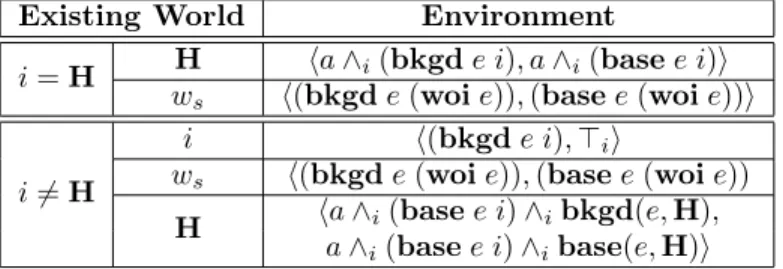
growl (sel ( x.¬(human x H)) >) H))) The above formula means that there is an accessible world j from the actual world H, in which a wolf walks in. And at the actual world, there is some individual that growls. But since the choice operator sel does not have a proper proposition from which it can pick up a referent, the anaphora in (13-a) cannot be resolved. Assume A is the proposition expressed by a wolf walks in, B is the one expressed by it
9Since we stick to the standard lexical entry of wolf (formula 4.33), its dynamic
entry (formula 4.34) does not indicate whether a wolf is human or not. We radically simplify this issue by assuming a powerful choice operator sel, which can resolve the satisfied variable by itself. However, an enriched lexical entry would be desirable in the future work.
Modal Subordination in Type Theoretic Dynamic Logic / 31
growls, M denotes the entry of might, then the possible worlds hierarchy of example (13-a) is depicted in figure 1:
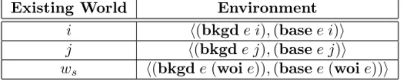
i ws j1 j2 j3 ... W A (mb ws)! A (mb ws)! A (mb ws)! A (mb ws)! A if i6= ws i j1 j2 ... if i = ws W A (mb i)! A (mb i)! A (mb i)! A
Figure 6: Possible Worlds Hierarchy ofJwouldKM -T T DLA
TTDL Lemma ?? P-TTDL Integrating M-TTDL
possible world
Figure 7: Relations between TTDL, P-TTDL, and M-TTDL
H j
M A B
A
Figure 8: Possible Worlds Hierarchy of Example ??
3
FIGURE1 Possible Worlds Hierarchy of Example (13-a)
The anaphor it occurs at world H, while the referent corresponding to a wolf is introduced in j. As a result, the anaphoric link cannot be resolved. It is the similar case for (13-b), although the detailed logical representation is different:
J(13-b)KM -T T DLnilistopiH
=J(13-b)-1KM -T T DL^mJ(13-b)-2KM -T T DLnilistopiH
⇣ 8s j.(R H j ! 9◆ x.(wolf x j ^ (walk in x j^
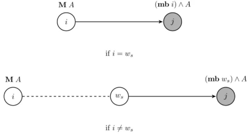
growl (sel ( x.¬(human x H)) >) H))) The above formula means that for all accessible worlds from the ac-tual world H, there is a wolf walking in at it. At the same time, there is some individual who growls at the actual world. But this growing indi-vidual cannot be properly resolved as any referent. Its possible worlds hierarchy is provided in figure 2:
H j1 j2 j3 ... W A B A A A A
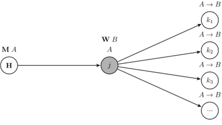
Figure 9: Possible Worlds Hierarchy of Example ??
H j k1 k2 k3 ... M A A W B A! B A! B A! B A! B
Figure 10: Possible Worlds Hierarchy of Example ??
4
FIGURE2 Possible Worlds Hierarchy of Example (13-b)
it occurs. Hence the anaphor is problematic.
Now let’s consider a more complex discourse concerning modal sub-ordination, where modalities are involved in both component sentences. It is in a parallel structure as example (6) in section 1.2:
(14) A wolfimight walk in. Iti would growl. (Asher and Pogodalla,
2011)
The first sentence of (14) is identical to (13-a)-1, hence: J(14)-1KM -T T DL=J(13-a)-1KM -T T DL
=JmightKM -T T DL(Jwalk inK(JaKJwolfK)) m
The representation for the second sentence can be achieved in a similar way:
J(14)-2KM -T T DL=JwouldKM -T T DL(JgrowlKJitK) m
Following the previous examples, the discourse incrementation for (14) is also straightforward. We will directly give the final result: J(14)KM -T T DLnilistopiH
=J(14)-1KM -T T DL^mJ(14)-2KM -T T DLnilistopiH
⇣ 9s j.(R H j ^ 9◆ x.(wolf x j ^ walk in x j^
8
s k.(R j k ! ((wolf x k ^ walk in x k) !
(growl (sel ( x.¬(human x k)) (wolf x k ^ walk in x k)) k))))) Now the choice operator sel will select a non-human variable at world
kfrom the proposition (wolf x k ^ walk in x k), where x is the only possibility. Hence we can further reduce the above formula as follows: J(14)KM -T T DLnilistopiH
⇣ 9s j.(R H j ^ 9◆ x.(wolf x j ^ walk in x j^
8
s k.(R j k ! ((wolf x k ^ walk in x k) ! (growl x k)))))
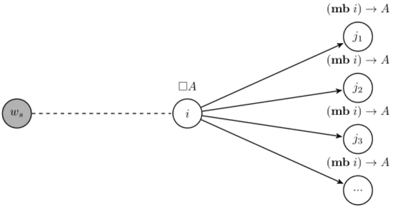
This means there exists a possible world j which is accessible from the actual world H, a wolf walks in at j; and at every accessible world kfrom j, if the wolf walks in, then it growls. This corresponds to the semantics of the original discourse (14). Again, we provide its possible worlds hierarchy as follows.
Finally, we will examine a last example, which switches back and forth between the modal mode and the factual mode. For the sake of convenience, we stick to the same vocabulary by simplifying example (18) from (Stone, 1999):
(15) A wolfimight walk in. John has a gunj. John would use itj to
Modal Subordination in Type Theoretic Dynamic Logic / 33 H j1 j2 j3 ... W A B A A A
Figure 9: Possible Worlds Hierarchy of Example ??
H j k1 k2 k3 ... M A A W B A! B A! B A! B A! B
Figure 10: Possible Worlds Hierarchy of Example ??
4
FIGURE3 Possible Worlds Hierarchy of Example (14)
We first have to compute the semantic representation for each com-ponent sentence. As we can see, (15)-1 is exactly the same as (13-a)-1 and (14)-1, we will not repeat it here any more. For the remaining two sentences, we have:
J(15)-2KM -T T DL=JhaveK(JaKJgunK)JJohnK m
J(15)-3KM -T T DL=JwouldKM -T T DL(JuseKJitK(JshootKJitK)JJohnK) m
The semantic representation of the whole discourse is obtained by straightforwardly sequencing the three component sentences with dy-namic conjunction. As before, we apply it to the empty left context nili,
the empty continuation stopi, and the world constant H. The reduced
J(15)KM -T T DLnilistopiH
= (J(15)-1KM -T T DL^mJ(15)-2KM -T T DL^mJ(15)-3KM -T T DL) nilistopiH
⇣ s9j.(R H j) ^ ( 9◆ x.(wolf x j) ^ ((walk in x j)^
(◆9y.(gun y H) ^ ((have john y H) ^ (((have john y j) ^ (gun y j))^
(8k.(R j k) ! ((((have john y k) ^ (gun y k)) ^ ((walk in x k) ^ (wolf x k))) ! (use
john
(sel ( x.¬(human x k))
(((have john y k) ^ (gun y k)) ^ ((walk in x k) ^ (wolf x k)))) (shoot
john
(sel ( x.¬(human x k))
(((have john y k) ^ (gun y k)) ^ ((walk in x k) ^ (wolf x k)))) k)
k))))))))
As we can see, both choice operators can select a non-human variable at world k from the sub-formula (((have john y k) ^ (gun y k)) ^ ((walk in x k) ^ (wolf x k)). Let’s assume the first sel picks up y, the second picks up x, then the above formula can be further reduced to:
J(15)KM -T T DLnilistopiH
⇣ s9j.(R H j) ^ ( 9◆ x.(wolf x j) ^ ((walk in x j)^
(◆9y.(gun y H) ^ ((have john y H) ^ (((have john y j) ^ (gun y j))^ (s8k.(R j k) ! ((((have john y k) ^ (gun y k))^
((walk in x k) ^ (wolf x k))) ! (use john y (shoot john x k) k))))))))
The semantics of the above complex formula is: there is a possible world j accessible from the actual world H, a wolf walks in at j; fur-thermore, John owns a gun at the actual world H; in addition, in every possible world k which is accessible from j, if the wolf walks in, then John uses the gun to shoot the wolf. As a result, all the anaphoric links in discourse (15), which are across the modal mode and the factual mode, can be correctly accounted for.
5 Conclusion and Future Work
Anaphora interpretation is a critical piece of machinery in natural lan-guage interpretation. The aim of this paper was to study the semantics of one specific type of anaphora: inter-sentential pronominal anaphora from the discourse perspective. More specifically, this paper was cerned with the phenomenon of modal subordination, and the
![[Book review] Neoliberal Governance and International Medical Travel in Malaysia by Meghann Ormond. Routledge, London, 2012, pp. xi + 162 (ISBN 978-0-415-50238-2).](data:image/gif;base64,R0lGODlhAQABAIAAAP///wAAACH5BAEAAAAALAAAAAABAAEAAAICRAEAOw==)