• Aucun résultat trouvé

Axisymmetric flame deconvolution using automated Tikhonov regularization

N/A
N/A
Protected

Academic year: 2021

Partager "Axisymmetric flame deconvolution using automated Tikhonov regularization"

Copied!
7
0
0

Texte intégral

(1)

Publisher’s version / Version de l'éditeur:

Vous avez des questions? Nous pouvons vous aider. Pour communiquer directement avec un auteur, consultez la première page de la revue dans laquelle son article a été publié afin de trouver ses coordonnées. Si vous n’arrivez pas à les repérer, communiquez avec nous à PublicationsArchive-ArchivesPublications@nrc-cnrc.gc.ca. Questions? Contact the NRC Publications Archive team at

PublicationsArchive-ArchivesPublications@nrc-cnrc.gc.ca. If you wish to email the authors directly, please see the first page of the publication for their contact information.

https://publications-cnrc.canada.ca/fra/droits

L’accès à ce site Web et l’utilisation de son contenu sont assujettis aux conditions présentées dans le site LISEZ CES CONDITIONS ATTENTIVEMENT AVANT D’UTILISER CE SITE WEB.

Combustion Institute Canadian Section, 2006 Spring Technical Meeting [Proceedings], 2006

READ THESE TERMS AND CONDITIONS CAREFULLY BEFORE USING THIS WEBSITE.

https://nrc-publications.canada.ca/eng/copyright

NRC Publications Archive Record / Notice des Archives des publications du CNRC :

https://nrc-publications.canada.ca/eng/view/object/?id=3dd02909-bbf4-42e2-9c58-2e00a9058bf4 https://publications-cnrc.canada.ca/fra/voir/objet/?id=3dd02909-bbf4-42e2-9c58-2e00a9058bf4

NRC Publications Archive

Archives des publications du CNRC

This publication could be one of several versions: author’s original, accepted manuscript or the publisher’s version. / La version de cette publication peut être l’une des suivantes : la version prépublication de l’auteur, la version acceptée du manuscrit ou la version de l’éditeur.

Access and use of this website and the material on it are subject to the Terms and Conditions set forth at

Axisymmetric flame deconvolution using automated Tikhonov regularization

(2)

Axisymmetric Flame Deconvolution using Automated

Tikhonov Regularization

K. J. Daun and K. A. Thomson

Institute for Chemical Process and Environmental Technology National Research Council of Canada

ABSTRACT

When deconvolving data collected in experiments involving axisymmetric flames, small errors that contaminate the data are magnified into large errors in the recovered distribution. Error magnification can be suppressed through Tikhonov regularization although a regularization parameter must first be identified, usually through a time-consuming trial-and-error procedure. This paper presents an algorithm that selects the regularization parameter automatically based on an estimate of the error contaminating the dataset. Solutions obtained using this algorithm are more accurate that those found by onion-peeling and Abel three-point deconvolution. Furthermore, because this algorithm selects the regularization automatically it is faster and easier to implement compared to the traditional trial-and-error regularization approach.

INTRODUCTION

The objective of many experiments involving axisymmetric flames is to deconvolve optical data measured along a set of chord lines passing through the flame field, called the projected data,

P(y), to recover the radial distribution of a field variable, f(r), over the range 0 ≤ r ≤ R, which is shown schematically in Fig. 1 (a). These two variables are related by Abel’s integral equation,

(1) a type of Volterra integral equation of the first kind. The simplest was of solving Eq. (1) is by onion-peeling. In this procedure the integral domain is first split into N evenly-spaced segments, which is equivalent to discretizing the flame field into N uniformly-spaced annular elements having a radial thickness ∆r = R/(N−1/2) as shown in Fig. 1 (b). By assuming that f(r) is uniform over each sub-domain of r, these values can be extracted from the corresponding integrals, which then contain only geometric terms. Carrying out these integrals transforms Eq. (1) into the N × N matrix equation AOPx = b, where xi = f(ri) = f(i∆r), bi = P(yi) = P(i∆r), and

(2)

This and other popular deconvolution techniques, including Abel three-point deconvolution, are described in greater detail in [1].

( )

( )

− = R y dr y r r r f y P 2 , 2 2

(

)

(

)

(

)

⎪ ⎪ ⎩ ⎪⎪ ⎨ ⎧ > ⎥⎦ ⎤ ⎢⎣ ⎡ + ∆ = − + ∆ < = . , 2 , 2 , 0 2 2 2 1 2 2 2 1 2 2 2 1 , OP i j i j i j r i j i j r i j A ij

(3)

Fig. 1: (a) Axisymmetric flame deconvolution and (b) discretization of the problem domain. Traditional deconvolution techniques provide accurate solutions for f(r) when the exact projected data is known. In an experimental setting, however, small errors that contaminate the projected data are magnified by deconvolution into large errors in the recovered field variable distribution. Error amplification is a consequence of the ill-posedness of Abel’s integral equation and increases with N, severely limiting the deconvolved field variable resolution. This is demonstrated in the test problem shown in Fig. 2. The field variable was first derived by fitting a 4th-order piecewise polynomial to normalized soot-volume fraction data from a line-of-sight attenuation (LOSA) experiment on a laminar flame [2]. The right-hand side vector b, which contains the projected data, was calculated by analytically integrating Eq. (1). This data was contaminated by a perturbation vector δb with elements randomly-sampled from an unbiased Gaussian distribution having a standard deviation of 0.01, which is typical of errors encountered in LOSA flame experiments [2]. Figure 2 shows that the small errors contained in δb are amplified by onion-peeling and Abel three-point deconvolution into large perturbations in the solution, δx.

TIKHONOV REGULARIZATION

Error amplification can be suppressed by using regularization to perform the deconvolution. Regularization techniques transform the original ill-posed problem into a set of better-posed or

regularized problems. Regularized problems that closely resemble the original ill-posed problem are themselves ill-posed, having solutions that solve the original problem with a very small residual but are also highly sensitive to small errors in the input data. Using more regularization improves the solution stability, but at the expense of solution accuracy. The degree of regularization is controlled by a regularization parameter, which is adjusted until an acceptable trade-off between solution accuracy and stability is obtained. In a recent work [3], we showed how Tikhonov regularization [4] can be used to perform axial flame deconvolution. In this approach the matrix equation obtained by onion-peeling is augmented by adding a homogeneous system of regularizing equations λL, where λ is a continuously-variable regularization parameter

(a) 0 ∆r = R/(N−½) 1 2 N−1 j = P(y) f(r) r y R (b) y y

(4)

and L is a smoothing matrix, which in this problem is an (N−1×N) matrix that approximates the derivative operator in discrete space [5],

(3)

The regularized solution, xλ, is the value of x that minimizes the residual norm of the augmented system of equations, i.e.

(4) which can be found efficiently by solving

(5) In our previous paper [3] we showed that λ can be adjusted with high fidelity until a near-optimum trade-off between accuracy and solution stability is found for a given field distribution, level of discretization, and degree of error contamination. Strategies for selecting λ are presented in the next section.

Fig. 2: Example LOSA deconvolution problem showing error amplification by deconvolution. (Based on experimental data from [2].)

(

ATOPAOP +λ2LTL

)

x =ATOPb. . 1 1 0 0 0 1 1 1 1 0 0 0 1 1 ⎥ ⎥ ⎥ ⎥ ⎥ ⎥ ⎦ ⎤ ⎢ ⎢ ⎢ ⎢ ⎢ ⎢ ⎣ ⎡ − − − − = L O O O M M O L L -0.4 -0.2 0.0 0.2 0.4 0.6 0.8 1.0 1.2 0.0 0.1 0.2 0.3 0.4 0.5 0.6 0.8 0.9 1.0 r, y f(r ), P(y) b b+δb x x+ δb (Onion Peeling) x+ δb (Abel Three-Point) 0.7 -0.6

(

)

, 0 2 2 2 ⎟ ⎟ ⎠ ⎞ ⎜ ⎜ ⎝ ⎛ ⎥ ⎦ ⎤ ⎢ ⎣ ⎡ − ⎥ ⎦ ⎤ ⎢ ⎣ ⎡ = − = −b x b x b x x x L A A A λ λ λ λ λ λ Min Min

(5)

SELECTING THE REGULARIZATION PARAMETER

When selecting the regularization parameter, the goal is to minimize the overall solution error, which is due to both the contamination of the projected data and to the regularization process. Formally, the total error is written as [6]

(5) where x denotes the exact, unperturbed solution, bpert = b+δb, xλpert = (x+δx)λ is the regularized solution of the perturbed matrix equation, and AOP−1 and Aλ−1 are the pseudoinverses of the onion-peeling and augmented matrices, respectively. The total error is more easily quantified by taking the l2-norm of the vectors in Eq. (5),

(6) where εreg(λ) is the regularization error and εpert(λ) is the perturbation error. As described above, increasing λ suppresses the magnification of δb and decreases εpert(λ), but this also increases the

εreg(λ) since λL obscures AOP in the augmented matrix Aλ as λ becomes large. Thus, a value of

λ must be chosen that is an acceptable trade-off between εpert(λ) and εreg(λ).

Most often, λ is selected heuristically with the aid of an L-curve [3, 6], a plot of the smoothed solution norm against the residual norm for solutions obtained using different values of λ. This curve is shown in Fig. 3 for the problem described above with N = 50. Although solutions on the far-left side of the curve have a small residual, ||AOPxλpert−bpert||2, they are under-regularized since their large solution norm, ||Lxλpert||2, shows that they are contaminated with large perturbations. Solutions become smoother as λ increases, but those on the far-right side of the curve are over-regularized because they no longer satisfy the original ill-posed problem as indicated by their large residual. The best trade-off between smoothness and accuracy is usually found by visually inspecting the solutions that lie near the corner of the L-curve, a time-consuming process that demands specialized knowledge of regularization on the part of the analyst.

A more sophisticated way of choosing λ is based on the observation that, since εreg(λ) and

εpert(λ) increase and decrease in a monotonic way with increasing λ, these errors can be balanced by using the value of λ that satisfies εreg(λ*) = εpert(λ*). Unfortunately, λ* cannot normally be found using Eq. (6) directly, since bpert is known rather than b and δb individually. An estimate of ||δb||2 is often available, however, usually from the variance of independently-measured sets of projected data. If this is the case λ† can be approximated using the discrepancy principle [6, 7], which states that λ should be chosen so that

(7) where δe is most often set equal to ||δb||2. The left- and right-hand sides of Eq. (16) are estimates of the regularization and perturbations error, respectively, projected into the vector space of b.

(

OP1 1

)

1 , 1 1 OPb b b δb x x− λpert =A− −A−λ pert = A− −A−λ −Aλ−

( )

(

)

( )

( ),

2 1 2 1 1 2 ε λ ε λ λ ε λ OP λ λ reg pert pert tot = − ≤ − + = + − − − δb b x x A A A , 2 2 OPxb = eδb pert pert δ λ A

(6)

Fig. 3: L-curve for the LOSA deconvolution problem shown in Fig. 2, with N = 50.

DEMONSTRATION OF METHOD

The performance of the Tikhonov auto-regularization method described above is compared to that of onion-peeling and Abel three-point deconvolution by solving the LOSA problem shown in Fig. 2. In order to simulate an experimental environment, the projected data is contaminated with error randomly-sampled from an unbiased Gaussian distribution having a standard deviation of0.01 20. Each element of the perturbed dataset, bpert, is set equal to the average of 20 independent samples, and the corresponding standard deviation of the mean, σm, is given by

20

σ , where σ is the standard deviation of the sampled data. The expected value of σm is 0.01, which is typical for LOSA experiments carried out on laminar flames [2].

The performance of the deconvolution algorithms is measured using the root-mean-squared error of the recovered field distributions,

(8) obtained using different numbers of projections, N. At each value of N, 20 independent sets of projected data are supplied to the deconvolution algorithms. The Tikhonov regularization parameter is calculated automatically for each dataset by substituting an estimate of ||δb||2,

(9) into Eq. (7), which in turn is solved for λ using a safeguarded secant root-finding algorithm [5]. The averages of the resulting εRMS values are plotted in Fig. 4, which shows that the solutions found using Tikhonov auto-regularization are superior to those found with onion-peeling and Abel three-point deconvolution over the whole range of N. In fact, the root-mean-squared errors

-0.6 -0.5 -0.4 -0.3 -0.2 -0.1 0 0.1 -4 -3.5 -3 -2.5 -2 -1.5 -1 -0.5 0 log10(||AOPxλ pert−bpert ||2) log 10 (| |Lx λ pert ||2 ) λ = 1.16 (over-regularized) λ = 0.004 (under-regularized) Increasing λ “Corner” of L-curve , 2 RMS N x xpert − = ε , 20 2 σ σ N N m = ≈ δb

(7)

of the Tikhonov solutions actually decrease with increasing N, because the perturbation error is suppressed to the extent that the dominant error in the Tikhonov solutions is caused by assuming a uniform f(r) over each element, which in turn diminishes with increasing N.

Fig. 4: Accuracy of field distributions obtained using different deconvolution techniques.

CONCLUSIONS

Tikhonov regularization is an effective way of solving flame deconvolution problems in which the projected data is contaminated with error. Implementation of this technique is complicated, however, by the fact that a regularization parameter must first be specified. This paper presented an algorithm for automatically selecting this value using the discrepancy principle. Tikhonov auto-regularization provides more accurate solutions than onion-peeling and Abel three-point deconvolution, and furthermore, because the regularization parameter is selected automatically, this technique is easier to implement than is the case when this value is found manually.

REFERENCES

[1] Dasch, C. J., Applied Optics 31:1146 (1992).

[2] Thomson, K. A., Güilder, Ö. L., Weckman, E. J., Fraser, R. A., Smallwood, G. J., and Snelling, D. R., Comb. Flame 140:222 (2005).

[3] Daun, K. J, Thomson, K. A., Liu, F. and Smallwood, G. J, Applied Optics (in press) [4] Tikhonov, A. N., J. Eng. Phys. 29:816 (1975).

[5] Press, W. H., Teuklosky, S. A., Vetterling, W. T., and Flannery, B. P., Numerical Recipes in C: The Art of Scientific Computing, 2nd Ed., Cambridge University Press, 2002.

[6] Hansen, P. C., Rank-Deficient and Discrete Ill-Posed Problems: Numerical Aspects of

Linear Inversion, SIAM, 1998.

[7] Morozov, V. A., Soviet Math. Dokl 7:414 (1966), as reported in [6]. 0 0.05 0.1 0.15 0.2 0.25 0 25 50 75 100 N εRMS Onion-Peeling Abel Three-Point Tikhonov Auto-Regularization

Figure

Fig. 1:  (a) Axisymmetric flame deconvolution and (b) discretization of the problem domain
Fig. 2:  Example LOSA deconvolution problem showing error amplification by deconvolution
Fig. 3:  L-curve for the LOSA deconvolution problem shown in Fig. 2, with N = 50.
Fig. 4:  Accuracy of field distributions obtained using different deconvolution techniques

Références

Documents relatifs

From this observation, it is expected that accurate results can be obtained if the trade-off parameters λ and the tuning parameters p and q are properly cho- sen, since

To address these problems, we propose a new model based on Bilateral Total Variation (BTV) regularization of the sharp image keeping the same regularization for the kernel.. We

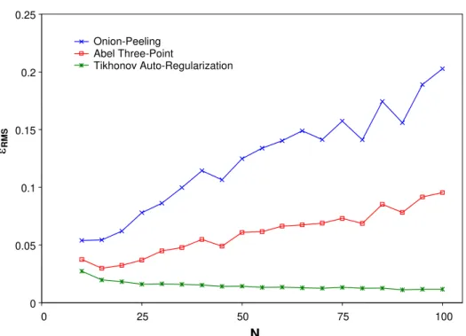
Since the normalized errors are of the same order of magnitude in both methods, we are tempted to claim that the minimization of I (3) , with the determination of the constant

The earliest occurrence and re- markable stasis of the family Bostrichidae (Coleoptera: Polyphaga) in Cretaceous Charentes

The Clink-induced increase in epidermal pavement cell and stomatal cell division and the concomitantly elevated level of ploidy of total nuclei from the corresponding leaves suggest

Objective of Report: This report investigates: (1) the actual and sustainable “Level of Investment” expenditures for maintenance of municipal infrastructure; (2) the extent of asset

In this section, we present an empirical comparison of the proposed estimators with classical approaches, namely Chebyshev polynomial approximation [16], and the conjugate gradient

L’enfant diabétique est exposé à deux complications métaboliques aiguës (hypoglycémies ou hyperglycémies avec acidocétose), pouvant être à l’origine d’un
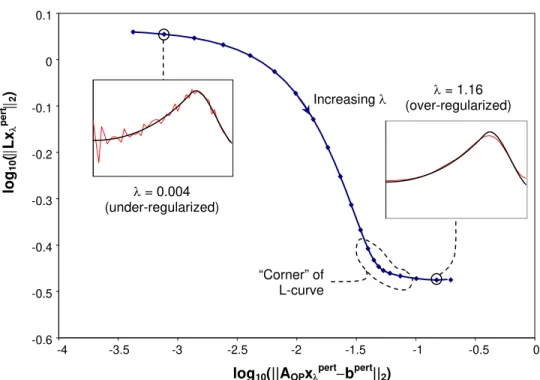